
Abstract
Following the introduction of the European Union Emissions Trading Scheme (EU-ETS), CO2 emissions have become a tradable commodity. As a regulated party, emitters are forced to take into account the additional cost of carbon emissions in their production costs structure. Given the high volatility in the carbon price, the importance of price risk management becomes unquestionable. This study is the first attempt that has been made to calculate hedge ratios and to investigate their hedging effectiveness in the EU-ETS carbon market by applying conventional, recently developed estimation models. These hedge ratios are then compared with those derived for other markets. In spite of the uniqueness and novelty of the carbon market, the results of the study are consistent with those found in other markets – that the hedge ratio is in the range of 0.5–1.0 and is still best estimated by simple regression models.
1. Introduction
Following the introduction of the European Union Emissions Trading Scheme (EU-ETS) in early 2005, emissions trading has officially become a reality. The EU-ETS is a legally enforceable market-based mechanism designed specifically to reduce greenhouse gas emissions (particularly carbon emissions). By making the price of the carbon allowance increasingly expensive, in the long term the scheme forces emitters to invest in alternative energy technologies, thereby achieving a gradual transition from a pollution-intensive industry to a cleaner, more sustainable industry.
There are several participants in the carbon market, the major ones being emitters, financial institutions, investors, market exchanges and the EU Commission. Each participant plays a different role: the EU commission is the regulator/policy maker, while emitters are the regulated parties. Trading is not limited to the emitters: investors (usually large corporations or financial institutions) are also permitted to take part. The purpose of the market exchanges and financial institutions is to facilitate the operation of the market. Accordingly, the impact on the introduction of emissions trading is expected to vary among these parties. The short- and long-term uncertainty for each party arising from the EU-ETS also differs from one industry to another.
From the policy makers’ perspective, they need to ensure compliance of the proposed trading scheme with the target set in the Kyoto Protocol. From an investor’s point of view, their uncertainty will be the portfolio risk and return after incorporation of the carbon allowances.
Undoubtedly, the emitters as the regulated parties are more affected than other market participants. To comply with requirements, emitters are forced to take into account the carbon allowance cost in their production cost structure. Similar to many other tradable commodities, prices of carbon allowances exhibit volatility, which should be dealt with by the application of appropriate risk management strategies. In the short run, risk management tends to focus on hedging, since no substitutes are available. Over the long run, hedging remains important and should provide more certainty to alternative energy investing. The transition from conventional ways of power generation to more environmentally friendly sources may take considerable time to implement. A sound hedging strategy would provide firms with more certainty (i.e. stability) over their production costs in the short term. Therefore, in the long term, they will have the ability to invest more confidently into alternative energy and other sustainable, clean technologies.
This paper aims to measure the optimal hedge ratio (OHR) in the EU-ETS carbon market using conventional and recently developed models of estimation. Based on variance reduction and utility improvement capabilities, the effectiveness of each estimated hedge ratio will be evaluated. The uniqueness of the paper rests in two areas. Firstly, this is an original estimation of the minimum variance hedge ratio as applied in the EU-ETS carbon market. Secondly, this is the first study to compare carbon market hedge ratios with other markets.
The EU-ETS carbon market is one that is new and unique. The underlying commodity in this market – carbon (represented by EUA - a unit of emission allowance), is one that is very different from those in the other financial markets (e.g. price fundamentals, nature and level of regulation), and one that is still not well understood. EUAs do not pay any interest or dividend, and the only potential cash flow from investment in carbon would be its resale price, which is in turn determined by expected market scarcity of carbon allowances (Benz and Truck, 2009). Like any other marketable asset’s price, the price of EUAs is determined by fundamental demand and supply. However, price determinants for carbon are unique. On the demand side, price may be determined by fuel prices, weather and economic growth, whereas on the supply side it is determined by the regulators, which is distinctive feature of the market (Seifert et al., 2008). Commentators such as Alberola et al. (2008), Rickels et al. (2007), Bonacina and Cozialpi (2009), Hintermann (2009), Mansanet-Bataller et al. (2007) and Uhrig-Homburg and Wagner (2008) confirmed the link between energy prices and EUA prices.
Hence, one might expect that existing finance theories, concepts and tools would not be applicable in this market. This is the main motivation behind this paper. The OHR, as an integral part of risk management, has been estimated in other financial markets: currency (Kroner and Sultan, 1993), stock index (Ghosh and Clayton, 1996), fixed-income (Ahmed, 2007), metals (Baillie and Myers, 1991), agriculture (Sephton, 1993) and power (Bystrom, 2003; Ripple and Moosa, 2007), among many others. In the carbon market, Chevallier (2008) studied Phase I of the EU-ETS extensively, with an emphasis on banking, pricing and risk hedging strategies. However, under the risk hedging section, the possible use of the OHR has not yet been discussed. Cetin and Verschuere (2009) proposed hedging formulas using a local risk minimization approach, but again, hedging with carbon futures contracts or other derivatives was not considered.
The distinctive, novel nature of the carbon market, however, provided a compelling motivation for us to re-estimate the hedge ratio in this market. The results showed that the magnitude and hedging performance of the OHR obtained for the carbon market are in line with those obtained for other markets. These results can be an indication that, in spite of the uniqueness of the carbon market, the tools, techniques, theories and concepts used in finance can still be applied in the analysis of such markets, subject of course to certain modifications. This should be a welcome development for financial market players such as institutional investors, portfolio managers and traders and speculators, as this should encourage them to participate in the carbon market.
This paper consists of six main sections. Section 2 provides an institutional setting for the EU-ETS carbon market. In Section 3, the concept of hedge ratios is introduced. In Section 4, the methodology of the estimation of hedge ratios in the carbon market is presented. Section 5 presents the estimation results accompanied by an extensive discussion. This is followed by a comparison of estimated hedge ratios in the carbon market to those obtained in other markets. The paper concludes in Section 6.
2. Institutional setting
The EU-ETS is the world’s largest multi-country, multi-sector mandatory greenhouse gas emissions trading regime, with 27 member states currently under the scheme. The regime covers CO2 emissions from electricity generation and the main energy-intensive industries, including power stations, refineries and offshore oil and gas production, iron and steel, cement and lime, paper, food and drink, glass, ceramics, engineering and auto manufacturing (Directive 2003/87/EC, 2003). Fundamentally, as a cap-and-trade program, the EU-ETS operates by placing a cap or limit on the amount of CO2 companies can emit every year. Each company is awarded an annual quota of carbon dioxide emission units where 1 unit of allowance = 1 tonne of CO2 (one unit of EUA). Firms that emit more than their allocated allowance can choose to pay the non-compliance penalty or purchase surplus allowance from companies that manage to stay below their limit. The system is designed to cut CO2 emissions in a cost-effective way. Over time the total number of quotas/allowances is to be reduced, which should lead to an increase in the price of carbon emissions allowances due to the enhanced scarcity of supply.
The allocation of EUAs is determined by each individual country’s Nation Allocation Plan (NAP). Each country designs its own NAP according to the emissions produced from different sectors and other relevant characteristics. Before distributing these allowances to firms and organizations, the NAP must be submitted to the EU Commission for approval.
Commencing operation in January 2005, three phases were set out in the EU-ETS: Phase I (2005–2007), Phase II (2008–2012) and Phase III (2013–2020). Phase I was an experimental scheme that started with six key industrial sectors: energy activities production, processing of ferrous metals, mineral industries and pulp, paper and board activities. In Phase II, coverage was broadened, so that in addition to Phase I, CO2 emissions from glass, mineral, wool, gypsum, flaring from offshore oil and gas production, petrochemicals, carbon black and integrated steel works were included. In Phase III, an EU-wide cap is proposed to replace the current system of NAPs set by each member state, and the overall cap will be further tightened on an annual basis.
Banking of allowances means that unused emission allowances are carried forward from the current year for use during the following year. Banking of allowances is permitted within Phases (except in France and Poland); however, this was prohibited from 2007 to 2008 (inter-phase). This had significant implications for the pricing of emission allowances and its underlying derivatives. However, industries are allowed to bank their unused permits from Phase II to Phase III. Financial penalties apply when emitters do not meet their compliance requirements. Moreover, all credit deficiencies must be purchased and, in addition, all fines must be paid. An independent third party is required to audit all the reported emissions.
There are currently three major market exchanges in operation to facilitate EU-ETS trading, namely the BlueNext, Nordpool and the European Climate Exchange (ECX). We use spot EUA contracts from BlueNext (based in Paris) and futures contracts from ECX (based in London) for hedge ratio calculations and effectiveness measurements. One lot of both the spot and the futures contracts covers 1000 tonnes of CO2 and there is a three-day delivery period after the trading day for futures contracts.
3. Hedging and hedge ratios
Hedging is an investment made to mitigate the price risk (or unfavourable fluctuation) of the underlying assets at maturity. A futures contract is a dominant instrument used in hedging, mainly because of its transparency and liquidity advantages over the others. Hedging is primarily implemented by using a hedge ratio, which determines the portions of the spot that need to be hedged in order to achieve a minimum level of unfavourable price fluctuation (Ederington, 1979; Johnson, 1960; Myers and Thompson, 1989).
Following Hatemi-J and Roca (2006), we define the OHR as the quantities of the spot instrument and the hedging instrument that ensure that the total value of the hedged portfolio does not change. It can be formally expressed in terms of the following:

where Vh is the value of the hedged portfolio, Qs and Qf are the quantity of spot and futures instrument, respectively, and S and F are the price of spot and futures instrument, respectively.


where h gives the hedge ratio.
Therefore, the hedge ratio can be demonstrated as the slope coefficient in a regression of the price of the spot instrument on the price of the future (hedging) instrument.
The type of hedge ratio depends on the objective function of the hedger. Minimum variance is the most popular and widely used approach, although this has been criticized for not taking into account the expected return, which is inconsistent with the mean-variance framework. Since the selection of a hedge ratio is dependent on the hedgers’ objective in the hedging position, this will be different for various participants in the carbon market. For example, investors need to protect the investment portfolio from carbon price risk while ensuring their returns at the same time. Therefore, the objective function of hedging under such circumstances should not be based solely on minimum variance. However, the objective of risk management for emitters in the market does not necessarily have to be the same as investors’ objectives. Because of its compulsory participation, priority should be given to hedging of the carbon price risk. Accordingly, the objective function for the emitters is likely to be (but is not limited to) the achievement of a minimum variance of the hedged portfolio.
4. Methodology and data
4.1. Data
The data used in this study consists of spot (cash) and futures contracts of the respective carbon trading instruments. One tonne of carbon dioxide permit equals one unit of EUA – the spot EUA data is drawn from the BlueNext exchange. In line with the Phases set by policy makers, our data is divided into two periods, which are referred to as BNS EUA 05-07 (Phase I BlueNext Spot EUA 05-07) from 24 June 2005 to 25 April 2008 and BNS EUA 08-12 (Phase II BlueNext Spot EUA 08-12) from 26 February 2008 to 18 December 2009. To match the hedging horizon and the maturity of the futures contract, the spot EUA dataset is subdivided into a number of periods.
Data on the futures contract is drawn from the ECX, known as the IntercontinentalExchange (ICE)/ECX EUA futures contract. ECX offers futures contracts on EUAs for different maturities; they are sorted as Dec-05, Dec-06, Dec-07, Dec-08, Dec-09, etc. To match the spot EUA data, this paper uses the ECX futures contract up to Dec-09 maturity. All spot and futures data mentioned above are historical daily closing prices.
To mitigate liquidity concerns, we have used the futures contract that is expiring at the nearest date. In Phase I of the EU-ETS, only contracts with a yearly expiration cycle were available for trade, whereas in Phase II, contracts that expire on a quarterly basis became tradable. However, the quarterly contracts in Phase II (i.e. Jan-08, Mar-08, Sep-08, Jan-09, Mar-09, Sep-09), are very illiquid with little or no trading volumes at all. Therefore, the most liquid contracts with yearly expiration for both Phases I and II hedge ratios estimation are used, with each contract from 2005 to 2009 maturing in December. Figure 1 demonstrates the historical trading volume of two contracts expiring in December 2008 and 2009, respectively.
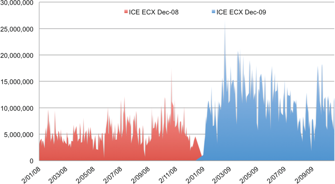
Intercontinental Exchange European Climate Exchange (ICE ECX) futures contract trading volume.
As shown in Figure 1, on average there are more than eight million tonnes of CO2 futures contracts being traded on a daily basis. With this clearly increasing trend of liquidity, the use of the Dec-08 and Dec-09 contracts should be sufficient to eliminate any liquidity concerns.
4.2. Hedge ratio estimation and evaluation of hedging effectiveness
This paper applies hedge ratio estimation models that have been widely used in calculating hedge ratios in other markets. These are the naïve approach, the ordinary least squares (OLS), the error correction model (ECM) and the generalized autoregressive conditional heteroscedasticity (GARCH) models.
4.2.1. Engle–Granger’s ECM
Assuming that St is BNS EUA or BNS CER spot,Ft is ICE/ECX EUA/CER Dec-xx futures contracts, the OHR is estimated as follows:
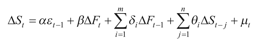
where β is the OHR,
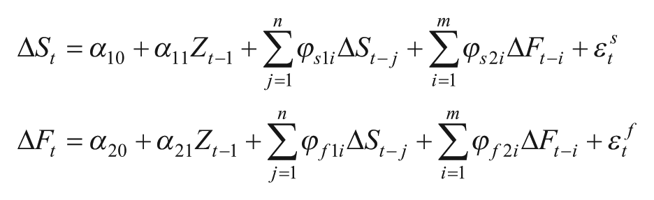
4.2.2. Vector error correction model
To incorporate the simultaneous determination of spot and futures in hedge ratio estimation, the vector error correction model (VECM) is implemented.
Firstly, let
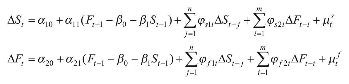
Thus:
where α 10α 20are intercepts, ϕ, α 11and α 21 are parameters and µ
t
s
µ
t
f
are white-noise disturbance terms.

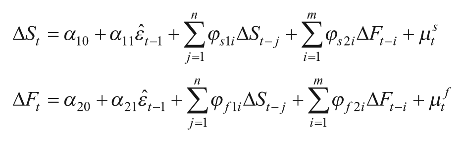
4.2.3. Vector error correction combining GARCH-BEKK
If we implement the GARCH error structure into the VECM, the following occurs:
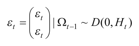
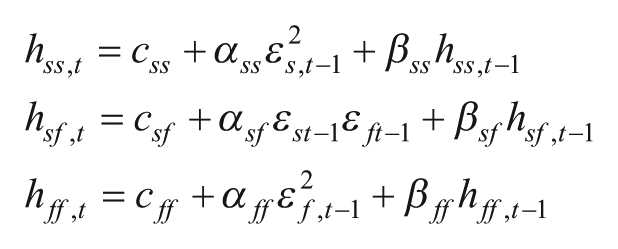
where Z is the error correction term, and ϵ t is the error term of the value at risk (VAR). Matrices A, B and C are parameter matrices and C is a lower triangular. The h* OHR is computed as

Thus, the minimum variance hedge ratio h* is time varying.
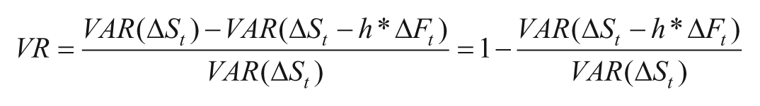
The effectiveness of each estimated hedge ratio is assessed based on two criteria popular in the literature: (a) Ederington (1979) variance reduction; and (b) utility maximization. There are several alternative measurements of hedging effectiveness applied in the literature, such as the certainty equivalent (CE; see Patton, 2004) and the adjusted information ratio (AIR; see Alexander and Barbosa, 2008).
To calculate the percentage variance reduction, the difference in variance of the unhedged portfolio and each hedged portfolio (constructed using different hedge ratios resulting from diverse models) is divided by the variance of the unhedged portfolio:
The utility maximization method incorporates the risk aversion of investors. Using this method, the level of investors’ utility that computed differently from the hedged portfolio is compared and ranked by the degree of utility improvement from the unhedged portfolio. This method now satisfies the mean-variance framework because it does not assess the minimum variance, but takes into consideration the return of the hedged portfolio. The objective function that maximizes the utility is given as
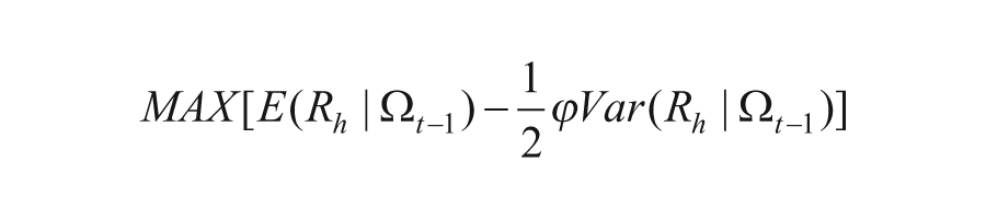
where Rh is the hedged portfolio (
The utility level for the hedged and unhedged portfolio is computed from the portfolio’s mean and variance of return.
5. Empirical results and discussion
5.1. Descriptive statistics and diagnostic tests
Table 1 provides the descriptive statistics for spot and futures of EUAs. Panel A reports the results on the original price level and panel B reports the returns level. Table 1 shows that all series are characterized by non-normalities.
Descriptive statistics.
Table 1 reports the descriptive statistics for the spot and the futures contract in various hedging horizons from 2005 to 2009 (Phase I of the European Union Emissions Trading Scheme covers 2005–2007 and Phase II starts from 2008 and ends in 2012). Panel A shows the results based on the raw data and Panel B reports the results based on the differenced data. The statistics reported are number of observations, mean, median, maximum, minimum, standard deviation, skewness, kurtosis, Jarque–Bera and probability.
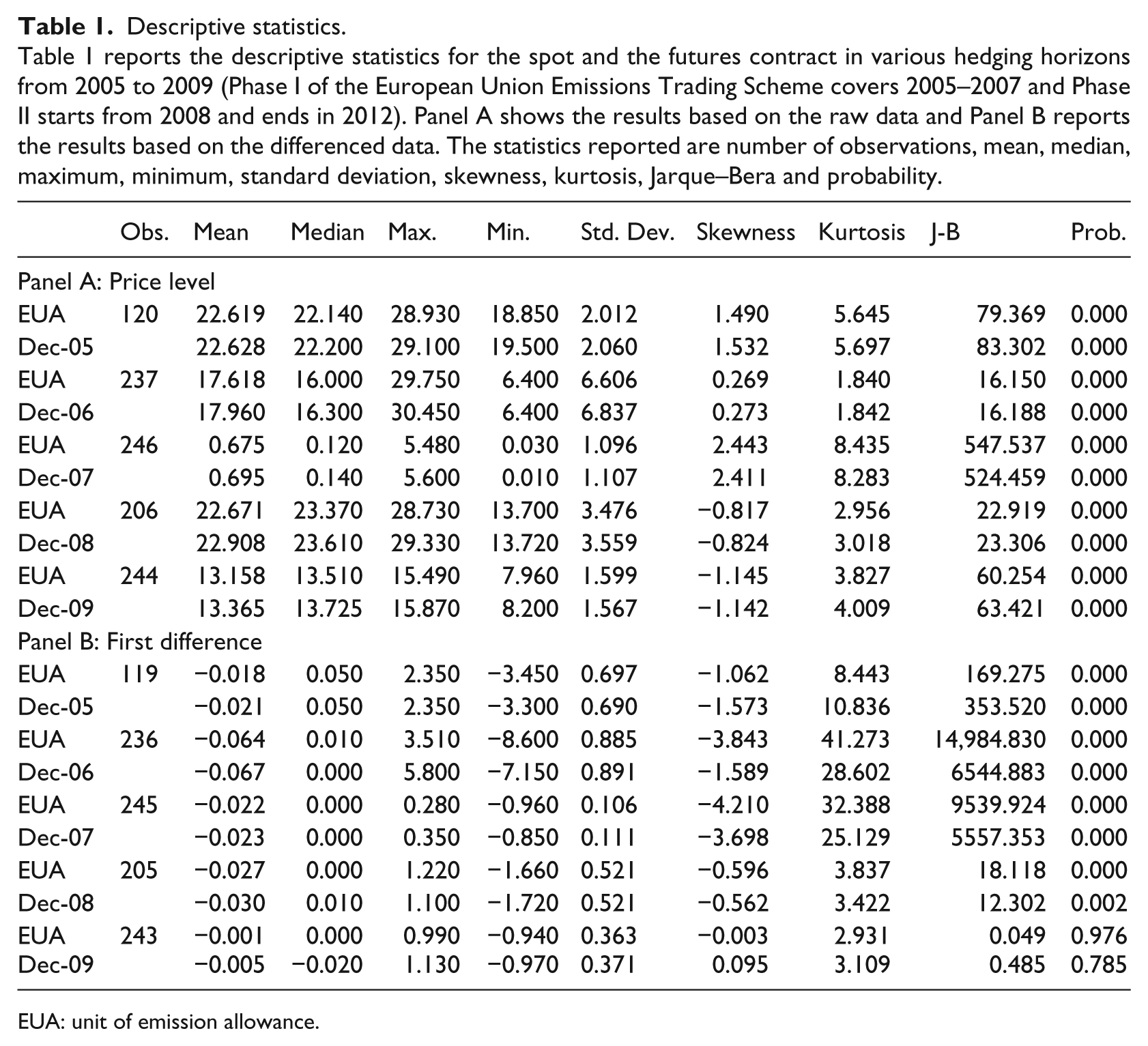
EUA: unit of emission allowance.
We tested for stationarity of each series based on the Augmented Dickey–Fuller (ADF) and Philips–Perron (PP) tests. We found that all series are non-stationary. We then conducted a co-integration test between the spot and future prices corresponding to different expiration dates – from December 2005 to December 2009 – using the Engle–Granger and the Johansen methodologies. The results show that the spot and future prices for all the different expiry dates are co-integrated (see Table 2).
Results of co-integration.
Following the Johansen’s technique, Table 2 shows the result of co-integration test between spot and futures from 2005 to 2009. The first column lists the test statistics and the second column specifies the number of co-integration equation. The test results are reported from the third column to the seventh column in comparison to the critical value at 5% level. The lag length is automatically selected and reported in the last row of the table.
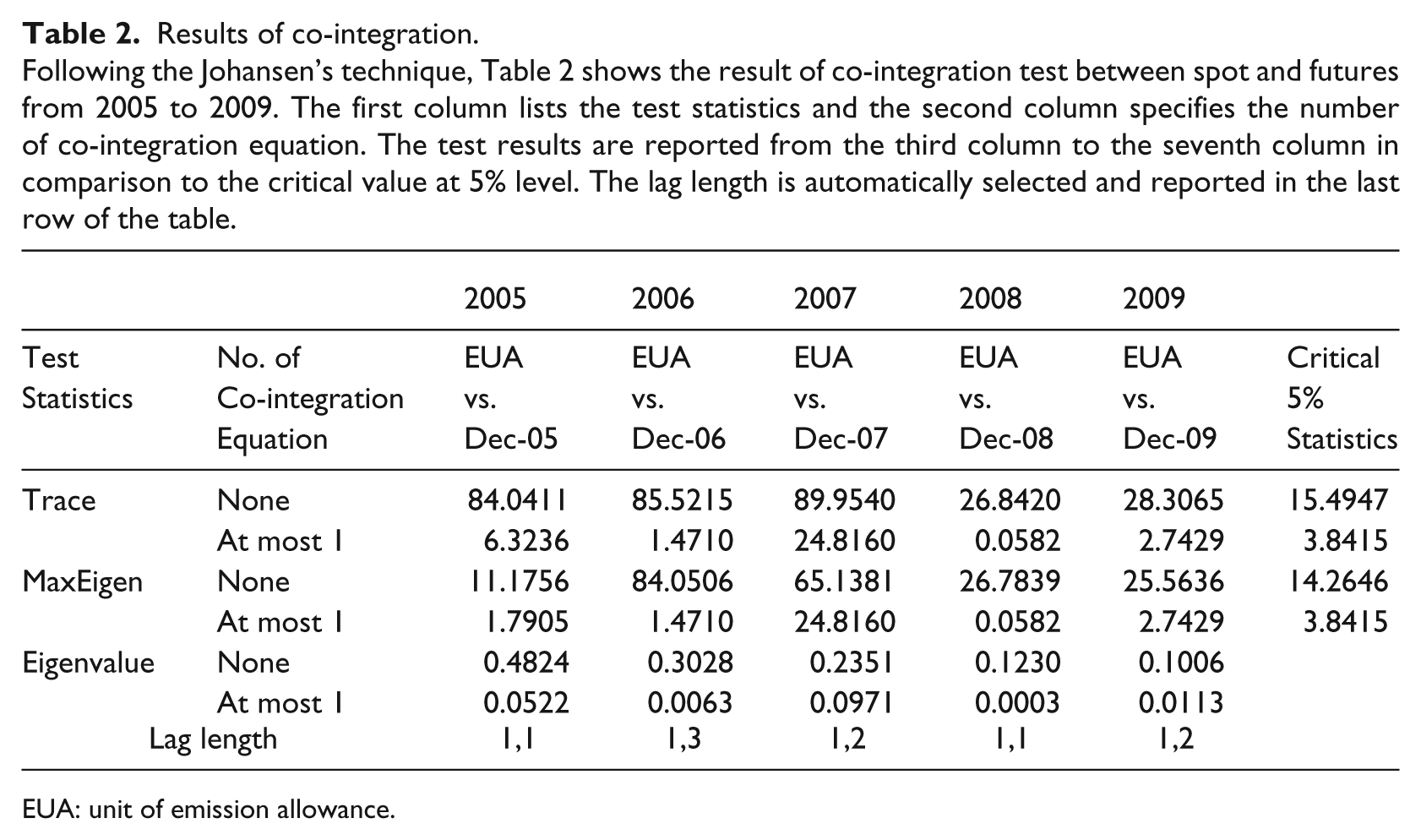
EUA: unit of emission allowance.
To ensure that the models are correctly specified, we tested for the lag length based on the Akaike Information Criterion and/or the Schwartz Information Criterion, conducted co-integration analysis, and checked for the stability of the VAR models. As mentioned above, the results of the co-integration and optimal lag length tests are presented in Table 2. 1
Meanwhile, the most obvious abnormal behaviour of the price series is observed from February to June 2006, when the sharp fall in price was recorded. Moreover, the near-zero price is seen at the end of Phase I. During the period of the sharp fall, the EUA price slumped by over 50%. The price stayed at around €15 for a few months, but then it declined continuously to its technical minimum of €0.01. This is recognized as the price collapse in Phase I of the EU-ETS. In Benz and Trück (2009), Chevallier et al. (2009), Alberola and Chevallie (2009), Alberola et al. (2008) and Daskalakis et al. (2009), it is commonly agreed that the publication of verified emission data during the previous compliance year was the major cause of this collapse. These reports indicated that emissions allowances were over-allocated to the emission-intensive firms, causing an excess supply of about 44 MtCO2 in the market. Towards the end of Phase I, the price dropped to a few cents, which was attributed to the banking prohibition of inter-phase EUAs. The fact that banking between phases was not allowed means that any surplus emission allowances could not be carried forward; therefore, they became worthless at the end of the Phase.
It is also worth noting that in Phase II of the EU-ETS, the price of EUA and futures dropped substantially from the start of July 2008 to early 2009 during the period of the Global Financial Crisis (GFC). The World Bank (2009) attributes this to the worldwide economic downturn, when demand for housing and cement, and automobiles and steel declined. Companies cut back their production, which in turn caused lower power consumption. As a consequence, emissions were lower and companies did not have to purchase allowances, since adequate free allowances were allocated to them prior to Phase II. On the contrary, companies that held excessive free allowances could choose to sell them in exchange for cash in a difficult credit environment, causing a decline in prices. From February 2009, following the economic recovery, the price of EUAs started to rise from its lowest level of €7.
During the global economic downturn, the demand for EUA hedging was expected to drop due to a lower production output. Following a bearish trend on the spot EUAs, emitters had no incentive to enter into the derivatives market. However, with the economic recovery, the price of EUAs was set to pick up again, and the demand for hedging was expected to increase. This is confirmed by the observations in Figure 1: the transaction volume on the EUA Dec-08 futures contract is clearly lower than on the Dec-09 contract.
5.2. Hedge ratios by different models in the EU-ETS carbon market
Table 3 contains a summary of hedge ratios for different hedging horizons sorted by models. Hedge ratios computed using Naïve, OLS, ECM and VECM models are time-invariant hedge ratios. All of them remain unchanged throughout the entire hedging horizons (i.e. Phase I and II). In contrast, since VECM-GARCH produces a time-varying hedge ratio, the results of VECM-GARCH reported in Table 3 are the averaged value of the dynamic, time-varying hedge ratios at each point in time, in order to allow these to be compared with hedge ratios obtained from the other models.
Calculated hedge ratios.
Table 3 reports the optimal hedge ratio (OHR) for each hedging horizon based on ordinary least squares (OLS), error correction model (ECM), vector error correction model (VECM) and VECM-generalized autoregressive conditional heteroscedasticity (GARCH). The first column outlines the European Union Emissions Trading Scheme Phase, followed by the hedging horizon in the second column. The third column indicates the respective futures contract used. The OHRs are reported from the fourth to the eighth columns.
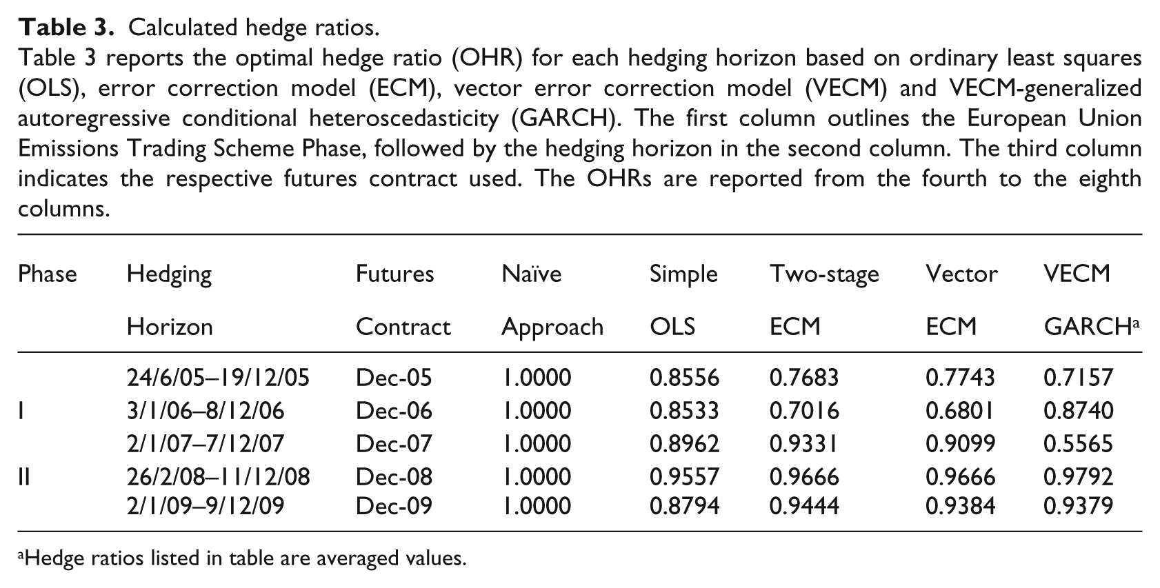
Hedge ratios listed in table are averaged values.
As can be seen from Table 3, hedge ratios (OHRs) vary from model to model and from period to period. Firstly, the calculated hedge ratios for the two-stage ECM and VECM are very close to each other in most cases. This is not surprising, given that they share the same error correction fundamentals. However, this minor difference may generate implications for hedge ratio performance evaluations, as OHR is one of the inputs for performance calculation. Secondly, in Phase II, all OHRs declined in 2009, compared to the 2008 hedging horizon. Thirdly, Phase II OHRs are generally greater than those of Phase I; this can be explained by the lower overall variance of futures price changes in Phase II as compared to Phase I.
5.3. Hedging effectiveness
5.3.1. Variance reduction
As evident from Panel A of Table 4, all models have produced significant variance reduction over the unhedged position across the entirety of Phases I and II hedging horizons. The smallest reduction is greater than 60% of the unhedged position. Meanwhile, the largest reduction (91%) indicates that it is close to a maximum-possible variance reduction. Thus, hedging with futures contracts has significantly reduced the risk (variance, in this case) of unhedged trading in spot EUAs.
Variance reduction based on different model.
Table 4 reports the results of variance reduction for each hedging combination achieved using the Naïve model, ordinary least squares (OLS) model, error correction model (ECM), vector error correction model (VECM) and VECM-generalized autoregressive conditional heteroscedasticity (GARCH) models. The first column outlines the European Union Emissions Trading Scheme Phase in accordance to the hedging horizon in the second column, which is followed by the respective futures contract used. The variance based on the unhedged or ‘no hedge’ position is reported in the fourth column. The hedge portfolio variances based on the Naïve model, OLS model, ECM, VECM and VECM-GARCH model are reported from the fifth to the ninth columns. The variance reduction for each hedging combination is presented in two rows. The first row represents the variance reduction in natural numbers, while the second row shows percentage variance reduction over the unhedged position. Panel A reports the in-sample results and Panel B reports the one-year-ahead out-of-sample results. The out-of-sample result is based on a one-year-ahead approach, where the 2005 OHRs are used to hedge the unit of emission allowance (EUA) price in 2006 and the 2006 OHRs are used to hedge for the EUA price in 2007.
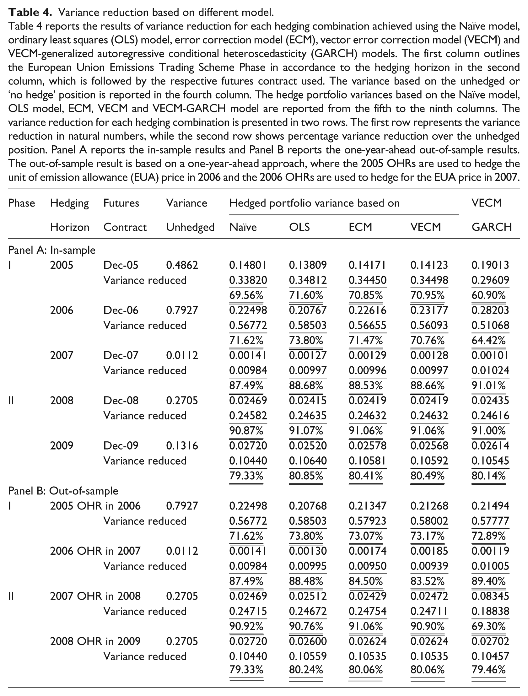
The one-year-ahead post sample results in Panel B show consistent results compared to Panel A in terms of variance reduction. All models achieved significant variance reduction in the out-of-sample periods. The minimum reduction is 69.30%, greater than the in-sample minimum, while the largest reduction is 91.06%, similar to the in-sample minimum reduction. However, the performance of individual hedge ratio estimation models is mixed; thus, a single conclusion on the superiority of a certain model cannot be drawn with confidence. Instead, general discussion on consolidation of the results is offered using a frequency distribution table. The performance of each model in terms of variance reduction is ranked within the seven hedging horizons (see Table 5).
Frequency distribution chart for ranking of variance reduction.
Table 5 reports the ranking of variance reduction obtained based on optimal hedge ratios (OHRs) derived by the Naïve model, ordinary least squares (OLS) model, error correction model (ECM), vector error correction model (VECM) and VECM-generalized autoregressive conditional heteroscedasticity (GARCH) model over the unhedged position. The first column lists the models employed for OHR computation. Ranks 1–5 indicate the frequency of each model being ranked at a specific level; the overall rank of each model can be found in the last column. The in-sample and out-of-sample ranking is reported separately in Panel A and Panel B, respectively.
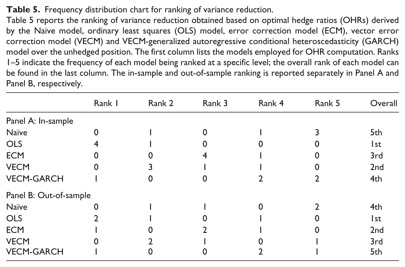
In contrast to some existing research, this study does not support the superiority of the VECM-GARCH model. As shown in Panel A of Table 5, the in-sample VECM-GARCH-generated OHR has been ranked the worst on two occasions. The conventional OLS is ranked as the best performing model in four cases, clearly outperforming all other models in overall ranking. The post-sample results appear to be generally consistent with the in-sample overall ranking where OLS outperforms the other models. The result came as no surprise, since Lien (2005a, 2005b) has shown that the Ederington model for hedging effectiveness favours OLS hedge ratios. Moreover, it is not surprising to see that frequency rankings and variance reduction of ECM and VECM are close to each other, since they share the same foundation of error correction mechanisms. Also notable in Tables 4 and 5 is that the difference in variance reduction between OLS and ECMs is relatively small (within 0.8%). The Naïve model, together with the VECM-GARCH model, is the worst performer in the overall ranking. Despite the difference in overall result, variance reductions achieved using Naïve, OLS and ECMs are very close to each other, with differences of less than 3.5% in all hedging horizons. Most notably, although the Naïve model provides a near-worst result, the variance reduction is not too far away from that of OLS and ECMs. This can be used as an argument for full hedge as the easiest hedging strategy. However, variance reduction achieved by the VECM-GARCH model in all Phase I hedging combinations appears to be much lower than the others (over 10% difference). In Phase II hedging combinations, such difference becomes much smaller.
Unlike a fixed OHR where the hedged portfolio remains unchanged across the hedging horizon, the VECM-GARCH model derived conditional OHR changes over time. Thus, the explicit transaction cost of rebalancing the hedged portfolio will have to be included if this is used in practice. Therefore, based on the result in this study (worst variance reduction) and taking into account transaction costs, the utility of VECM-GARCH in the EU-ETS market over the studied period is seriously questioned. Such findings are in line with Bystrom (2003), Copeland and Zhu (2006), Lien et al. (2002) and Moosa (2003), where OLS was found to outperform the more complex and sophisticated models. Later, in Lien (2007), it is shown that, in large sample cases, the conventional hedge ratio provides the best performance, whereas for small sample cases a sufficiently large variation in the dynamic variance of the futures return is required in order for dynamic models to produce favourable variance reduction. It is also worth noting that the hedging effectiveness measure is based upon the unconditional variance. The conventional hedge ratio aims to minimize the time-invariant variance, while the conditional hedge ratio attempts to minimize the dynamic variance.
These findings are in line with the theoretical contributions of Lien (2005a, 2005b), who convincingly proved that OLS hedging effectiveness is expected to outperform other hedging ratios when the Ederlington measure is used. Exceptions are when there is a structural break in the data, which was the case in this study in 2007 and 2008 with the transition from Phases I and II, where ECM-based models produced superior results. Lien (2005a, 2005b) proposes the use of the residual variance of the hedged portfolio instead; however, empirical tests using this strategy are yet to be seen. The pure variance reduction approach of performance evaluation is criticized for not taking utility into account; therefore, the next section incorporates the utility factor into the modelling.
5.3.2. Maximum utility
Adopting the procedures discussed in the methodology section, Table 6 provides the utility improvements that have resulted from using different models with a risk aversion ranging from 1 to 3. Results of each hedging horizon are reported separately in chronological order. Similar to variance reduction, the utility improvement over the unhedged position is presented both in natural numbers and percentages. Panel A reports the in-sample results and Panel B reports the out-of-sample results.
Utility improvement based on different models.
Table 6 shows the results of utility improvement over the unhedged position based on the Naïve model, ordinary least squares (OLS) model, error correction model (ECM), vector error correction model (VECM) and VECM-generalized autoregressive conditional heteroscedasticity (GARCH) models. The table is divided into two panels where Panel A reports the in-sample results and the one-year-ahead out-of-sample results can be found in Panel B. In each panel, there are three blocks of results. The first block represents the result of risk aversion level 1, followed by the results based on risk aversion level of 2 and 3. Similar to Table 4, the first column of the table outlines the hedging horizon followed by the respective futures contract used. In addition, utility of the unhedged position and the utility improvement over the unhedged position are reported in each block based on different risk aversion levels.
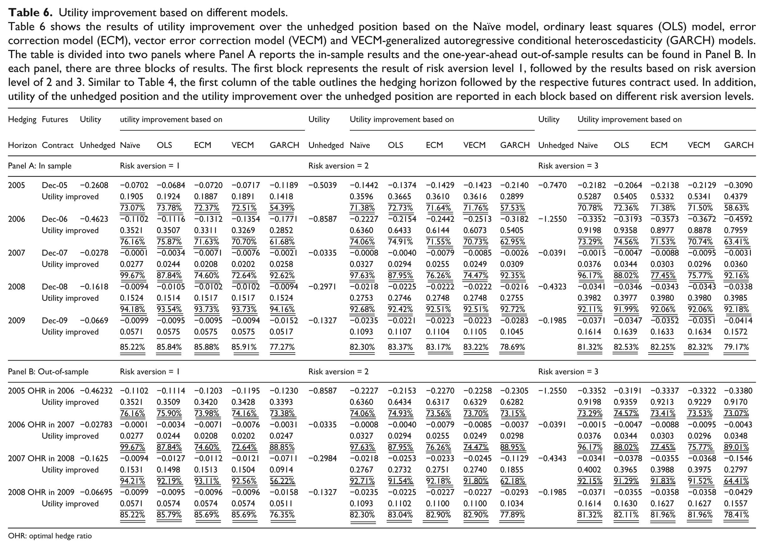
OHR: optimal hedge ratio
As can be seen in Table 6, under different levels of investor’s risk aversion, the results of utility improvement achieved by different models are mixed. Table 7 reports the frequency distribution of the utility improvement rankings under the risk aversion ranging from 1 to 3.
Frequency distribution chart for ranking of utility improvement.
Table 7 reports the ranking of utility improvement obtained based on optimal hedge ratios (OHRs) derived by the Naïve model, OLS model, error correction model (ECM), vector error correction model (VECM) and VECM-generalized autoregressive conditional heteroscedasticity (GARCH) model over the unhedged position. Panel A shows the in-sample results, while Panel B reports the out-of-sample utility improvement rankings. The first column of Table 7 outlines the list of models used for OHR computation. Ranks 1–5 indicate the frequency of each model being ranked at a specific level (i.e. from the best of 1 to the worst of 5). Based on risk aversion levels of 1–3, the overall rank of each model can be found in the ‘overall’ column.
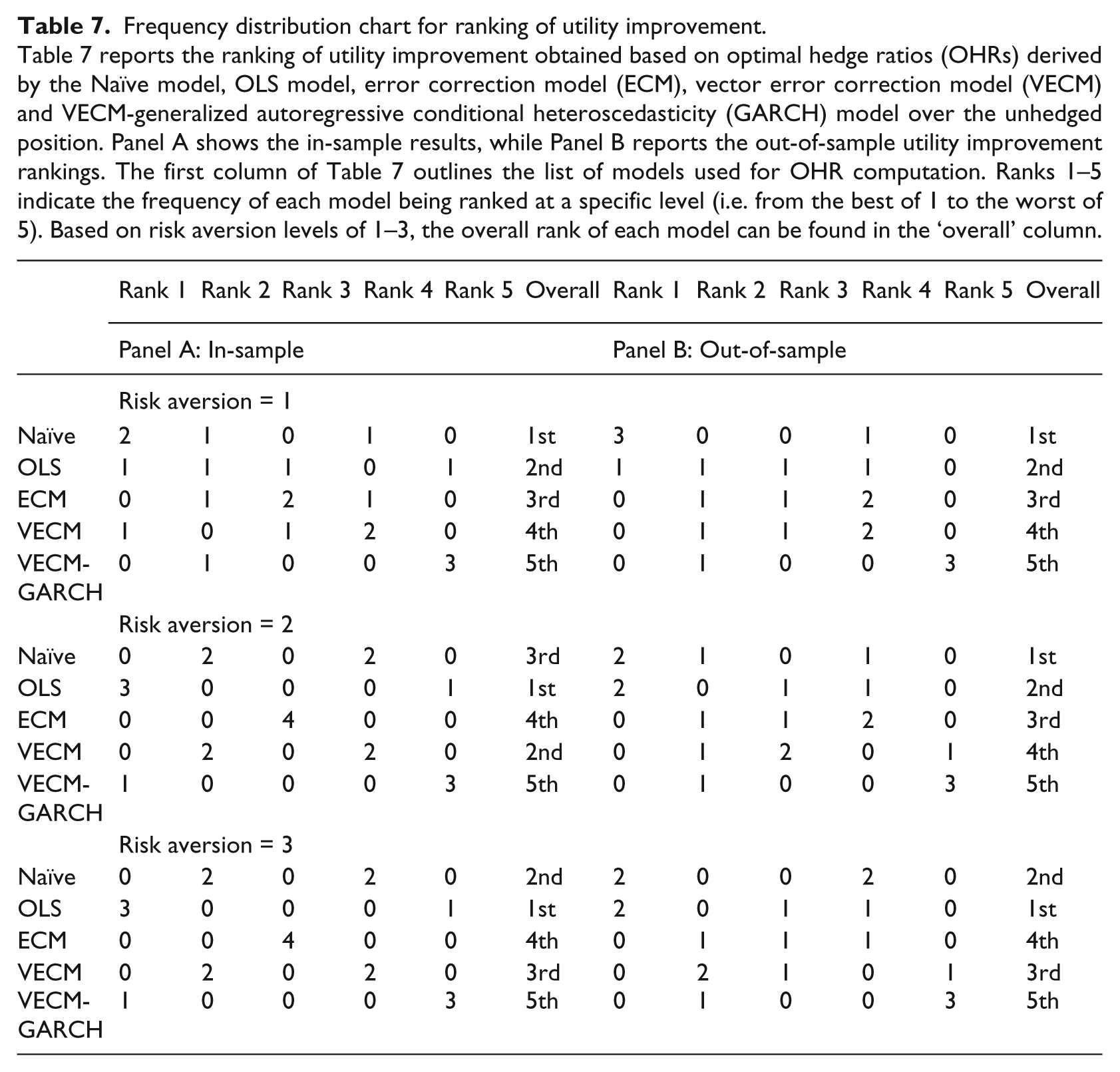
As observed in Panel A of Table 7 with risk aversion set at 1, the model that most frequently produces the highest utility improvement over the unhedged position is the Naïve model. Under risk aversions 2 and 3, OLS demonstrated the best overall performance. This result confirms findings based on variance reduction capabilities, which in turn suggests robustness of the findings. However in a one-year post-sample world, the Naïve model demonstrates superiority in utility improvements regardless of risk aversion levels. Nevertheless, the OHR derived by VECM-GARCH consistently produces the lowest utility improvement at all levels of risk aversion in both in-sample and out-of-sample performance rankings. The findings presented in Table 7 further confirm the poor hedging effectiveness of the VECM-GARCH-derived hedge ratio in the carbon market setting.
Furthermore, when comparing in-sample and out-of-sample hedging effectiveness, it is important to take note of some of the limitations encountered in this study that are not common in other markets. Firstly, because Phases I and II operated under different regulatory environments, the results of Phase I hedge ratios used for calculation of out-of-sample effectiveness in Phase II should be treated with care. Secondly, due to the price collapse at the end of 2006, the price in the entire 2007-hedging horizon was around zero. Again, this largely discounts the meaningfulness of using the 06-hedge ratio for 07 out-of-sample tests. As a result, only data from the years 2006 and 2009 provide economically meaningful post sample estimates. Finally, in 2005 and 2006 we had to overcome problems with the varying number of observations in each hedging horizon, which created difficulties for computations of out-of-sample effectiveness when using GARCH hedge ratios. The 2009 hedging horizon was the only one where no significant problems were encountered.
5.4. Comparisons of carbon hedge ratios to those in other markets
Due to the peculiarity of the carbon market, we also compared the carbon hedge ratios with those estimated in other markets. Table 8 lists hedge ratios derived using OLS model, ECM and GARCH model in various existing markets. It should be noted here that the hedge ratios in the GARCH column are presented as averages. These ratios are then compared with EUA versus Dec-09 hedge ratios with the hedging horizon from 2008 to 2009 up to 20 December 2009.
Comparison of carbon hedge ratios with those in other markets.
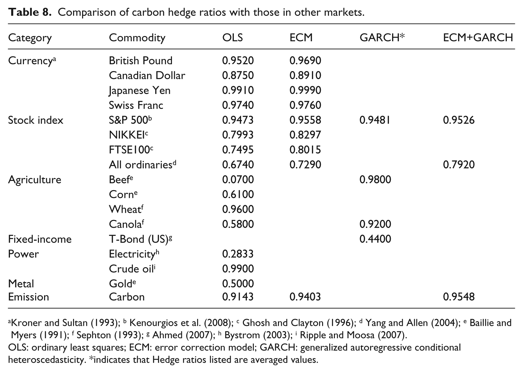
Kroner and Sultan (1993); b Kenourgios et al. (2008); c Ghosh and Clayton (1996); d Yang and Allen (2004); e Baillie and Myers (1991); f Sephton (1993); g Ahmed (2007); h Bystrom (2003); i Ripple and Moosa (2007).
OLS: ordinary least squares; ECM: error correction model; GARCH: generalized autoregressive conditional heteroscedasticity. *indicates that Hedge ratios listed are averaged values.
It can be observed that all ratios lie within the range of 0.5–1 with the exception of some of the GARCH conditional hedge ratios. For example, in Baillie and Myers (1991), the hedge ratio for beef was found to have zero variance reduction; therefore, it is not recommended for hedging application. This was later confirmed by Yang and Awokuse (2003), where the hedge ratio for live cattle did not produce much variance reduction compared to no hedge at all. Hedge ratios for carbon emissions are listed last in the table. Despite its special features, the size of the carbon hedge ratios is not so different from that of other markets.
6. Conclusion
This paper investigated a number of approaches towards the estimation of the OHRs in the EU-ETS carbon market, including the Naïve model, OLS model, ECM, VECM and VECM-GARCH model. Significant reduction of volatility can be attained if spot positions are hedged in futures markets independently of the hedge ratio estimation method that is applied. However, the performance of the models was not uniform. For example, the findings from this paper do not favour the use of the VECM-GARCH model for the hedging of EUA price risk. If the emitter chooses the minimum variance as the objective, the hedge ratio calculated by OLS estimation should be selected, as it provides the greatest variance reduction compared to other models. However, if the hedger (not limited to emitters) expects to incorporate the return as well as minimum variance, a choice between the OLS model, Naïve model and ECM can be made. As suggested by the findings of this research, the results in terms of utility improvement are quite mixed in different hedging horizons. Again, VECM-GARCH model results did not produce encouraging results in terms of overall utility improvement. When comparing values of hedge ratios with hedge ratios obtained in other markets, no significant differences were found. Thus, in spite of the uniqueness and novelty of carbon markets, the estimated hedge ratios also fall in the range of 0.5–1, in line with those of other markets.
There are some limitations in this study that warrant future research. For example, once the full data for Phase II becomes available, better analysis and more accurate estimations will be possible. The structural break in Phase I of the EU-ETS is not comprehensively modelled and tested in this paper. To incorporate this, other studies have used dummy variables to represent such phenomenon. Ultimately, from the portfolio manager’s perspective, the asset allocation problem and portfolio optimization can be revised after incorporating carbon instruments. Thus, management of risk and return on such revised portfolios becomes essential for possible future research.
Footnotes
Acknowledgements
The authors thank the anonymous referee for providing us with valuable comments. The paper has benefited from discussions with Adrian Cheung, Jen-Je Su, Nicholas Rohde, Robert Bianchi and Michael Drew. We would also like to thank participants at the Finance Writing Retreat 2009 held at Griffith University and the 2010 Finance, Accounting, Investment and Risk Management (iFAIR) Conference held at Southwest Jiaotong University, Chengdu. The scholarship and travel grant provided by Griffith Business School and Department of Accounting, Finance and Economics are greatly acknowledged. All errors are our own.
Date of acceptance of final transcript: 18 October 2012.
Accepted by Associate Editor, Garry Twite (Finance).
Funding
This research received no specific grant from any funding agency in the public, commercial or not-for-profit sectors.