Are Activity Patterns Stable or Variable? Analysis of Three-Year Panel Data

Abstract

Routines and mandatory activities, such as work and school, shape the activity patterns of individuals and strongly influence travel demand. Knowledge about stability and variability of these routines could strengthen travel demand modelling and forecasting. A longitudinal perspective is required to investigate these aspects. In this study, the activity patterns of a sample of people is compared for one week in two successive years. It is analyzed whether the activity patterns of a given person vary from year to year, to what degree, and how this variability and stability can be measured. It is considered whether socio-demographic factors and life events determine stability in weekly activity patterns. The study is based on the representative panel survey, German Mobility Panel. The weekly activity patterns of the same respondents in different years is assessed, using two methods to measure stability and variability. The survey respondents are clustered into three groups according to the degree of variability in their activity patterns. A logistic regression model is also used to identify socio-economic and demographic covariates for similarity in weekly activity patterns. Results show that about one-third of the sample had the same or very similar weekly activity patterns in the two years examined. A person’s occupation status is a good predictor for the variability of activity patterns. Moreover, persons undergoing a change in occupation status are quite likely to show a greater variability in their activity patterns.

Routines and mandatory activities, such as work and school, shape the activity patterns of individuals and strongly influence their travel behavior. To investigate the stability or variability of these routines, a longitudinal time perspective is required. Understanding stability and variability in travel behavior and activity execution is, in turn, essential for developing rational planning policies and forecasting travel demand ( 1 – 3 ). Therefore, various research methods have been applied to address this issue. When describing behavior at different points in time, one can choose from several terms. These include “habits and routines,”“rhythmic patterns,”“stability,” and “variability” ( 1 , 2 , 4 – 6 ).

In this study, the activity patterns on an intra-personal basis are analyzed in different weeks of different years. The term stability is used to describe a constant behavior and variability to describe a changing behavior. Since variability is the opposite and thus not stable, the term “stability” is also used to refer to the measurement of both. Scope is not limited to day-to-day differences in behavior but behavior investigated for a whole week in two different years. Furthermore, the focus is on activity patterns found in the two survey weeks. The combination of longer time periods and the focus on activity patterns is an under-explored research field. By analyzing behavior from year to year, it can be explored whether changes in activity patterns result from life events, such as changes in occupational status or residence. The research questions are: Do the activities of the same individual differ from year to year? If so, how much, and how can stability in activity patterns be measured? Which socio-demographic factors and life events determine stability in weekly activity patterns?

The study draws on data from the German Mobility Panel (MOP), a representative panel survey of everyday travel in Germany. The weekly activity patterns of the same respondents who participated in the panel survey in different years between 2005 and 2015 is assessed. Activity patterns from trip diaries of the MOP are identified and two methods introduced to measure the stability of these patterns. Based on these measures, survey participants are then divided into three similarity groups according to the stability of activity patterns between weeks.

The paper is structured as follows: First, the existing literature on behavior stability and on the distance measuring methods used in behavior analysis is reviewed. Second, the paper describes in more detail the methodology sketched briefly above. Third, results are presented for the different activity patterns and distance measures. Finally, a logistic regression model is used to identify socio-economic and demographic covariates for similarity in weekly activity patterns.

Literature Review

The idea of measuring similarity has its origins in biology, in which two DNA strings or protein sequences must often be compared. When using distance measures, one generally calculates the similarity between two sequences. For alphabetical strings, two standard distance measures are widely used in research: the Hamming distance ( 7 ) and the Damerau-Levenshtein distance ( 8 ). Whereas both distance measures quantify similarities between two strings, the Hamming distance is more appropriate for sequences of equal length ( 8 ).

Over time, the basic idea of similarity measurement was refined and adapted for different research fields, such as computer science and transportation. The resulting methods are often referred to as sequence alignment methods. (For an extended overview, see Hosangadi ( 8 ) and Joh et al. ( 9 ).) The measurement of similarity has become increasingly important in transportation research. For example, distance measures are used to analyze mode choice, activity patterns, activity departure times, or some combination thereof ( 2 – 4 , 10 – 18 ). Joh et al. ( 9 ) divided the methods used in travel behavior research into three groups. The first examines the composition of elements in two or more activity patterns to find differences. Here, the corresponding characters of two patterns are compared ( 19 ). The second considers element composition and sequence, but compares each element separately. The third consists of multidimensional sequence alignment that considers element composition and the sequence of the activities through simultaneous comparison ( 9 ). Wilson ( 11 ) introduced the use of sequence alignment to assess the stability of daily activities by translating activity patterns into a sequence of characters. This led to further developments in multidimensional sequence alignment methods with advanced applications and complex sequence structures ( 9 ).

Some research deals with classification studies, which identify interpersonal similarities by comparing activity patterns within a certain period ( 10 – 12 ). Other researchers ( 3 , 9 ) have examined an individual’s activity patterns from day to day within the same week and found significant variability in travel behavior. Most of these studies do not capture variability over long periods, such as weeks or years, however, since they are based on cross-sectional studies using travel diaries limited to a maximum of two days. Only a few studies use longitudinal surveys to capture variability. Cherchi & Cirillo ( 1 ) and Schlich ( 3 ), for example, use the 6-week Mobidrive survey to compare the corresponding weekdays of different weeks in the same year. Bargeman ( 10 ) investigates variability in tourism travel behavior over several years by means of vacation histories. Cherchi & Cirillo ( 1 ) define tours with associated activities and modes. Based on these tours, logit models were developed to identify the factors impacting day-to-day variability in mode choice within a week ( 1 ). Raux et al. ( 2 ) investigate temporal rhythms in activity patterns and estimate influences on those variations.

In reviewing previous literature, however, no evidence is found of an intrapersonal day-to-day or week-to-week comparison between two years of panel data. Moreover, only a few studies investigate the relevant parameters that influence stability in activity patterns or mode choice. Further research on year-to-year stability in travel behavior is clearly needed, since longer periods can better capture the changes in life situation that typically influence behavior. In this paper, panel data is used to help close this research gap by studying the stability of activity patterns across two weeks located in different years.

Data

The study draws on travel survey data from the German Mobility Panel. This section gives an overview of the panel and introduces the study sample.

The German Mobility Panel

The German Mobility Panel (MOP) is a German National Household Travel Survey (NHTS) that has been conducted each year since 1994. It is carried out on behalf of, and funded by, the German Federal Ministry of Transport and Digital Infrastructure. The market research firm KANTAR TNS is responsible for the field work (i.e., recruitment and data collection) and the Institute for Transport Studies of the Karlsruhe Institute of Technology is in charge of the survey’s design and scientific supervision ( 20 , 21 ). The MOP survey is conducted each autumn and, since the aim is to track everyday travel, the survey weeks are chosen to avoid school and bank holidays. The participants provide a complete trip diary for an entire week. This contains information about all their trips during a whole week, that is, distances traveled, means of transportation, trip purposes, and start and end times. Information about the socio-demographics of the participants, the availability of cars and bicycles, and the possession of transit passes is also collected. Participants also indicate whether the trip diary period was typical or non-typical, for example, whether they were ill or on holiday.

The sample size is 1,000 to 1,700 households containing 2,000 to 2,700 persons (aged ten years and older). The MOP is a rotating panel survey, and participants are asked to take part for three consecutive years. Each year, a portion of the households is dropped from the subsequent wave and replaced with new households.

Study Sample

The sample used for analyses is based on data collected between 2005 and 2015. This data contains 7,685 persons from 5,089 households that participated at least once during these years. They reported over 311,000 trips. Since the study focuses on year-to-year differences in activity patterns, only people that participated for at least two years in a row were of interest to the study. Those survey participants reporting non-typical periods such as illness or vacation were also removed from the sample since these diaries may have captured atypical behavior instead of behavioral change—the goal of the study. The final study sample contained 2,573 participants from 1,983 households. To review changes between two years, 3,491 transitions were ultimately used;2,573 between participants’ first and second year participation and 918 between their second and third year participation.

Methods

To compare activity patterns from different years, first it is shown how activity schedules are generated from trip diary data. Next, it is explained how patterns are derived from those schedules and the measures to estimate differences between them are introduced. Finally, the logistic regression method used to further interpret the data is shown.

Data Transformation

To compare the activity patterns of people, activity data is needed. Since the MOP survey contains a trip diary, the activities (i.e., what people do between trips) can be inferred indirectly from the dataset only. Table 1 shows a one-day example of the transformation from trip data (left side—result of the survey) to activity data (right side—result of inference). For this transformation, it is assumed that people start their trip diary at home on the beginning of the first day. The analyses differentiate between the following activities: work, education, leisure, shopping, transport (pick-up, drop-off), and being at home. Detailed information about the activities a person performs at home was not queried in the MOP survey.

Table 1.

One-day Example: Trip Diary and Inferred Activity Diary

Trip diary			Inferred activity diary
Start	End	Purpose	Start	End	Purpose	Tour number	Tour purpose
			midnight	8:00 a.m.	Home	-	-
8:00 a.m.	8:30 a.m.	Work	8:30 a.m.	12:15 p.m.	Work	1	Work
12:15 p.m.	12:20 p.m.	Leisure	12:20 p.m.	1:10 p.m.	Leisure	1	Work
1:10 p.m.	1:15 p.m.	Work	1:15 p.m.	4:30 p.m.	Work	1	Work
4:30 p.m.	5:00 p.m.	Home	5:00 p.m.	7:00 p.m.	Home	-	-
7:00 p.m.	7:15 p.m.	Shopping	7:15 p.m.	7:45 p.m.	Shopping	2	Shopping
7:45 p.m.	8:00 p.m.	Home	8:00 p.m.	11:59 p.m.	Home	-	-

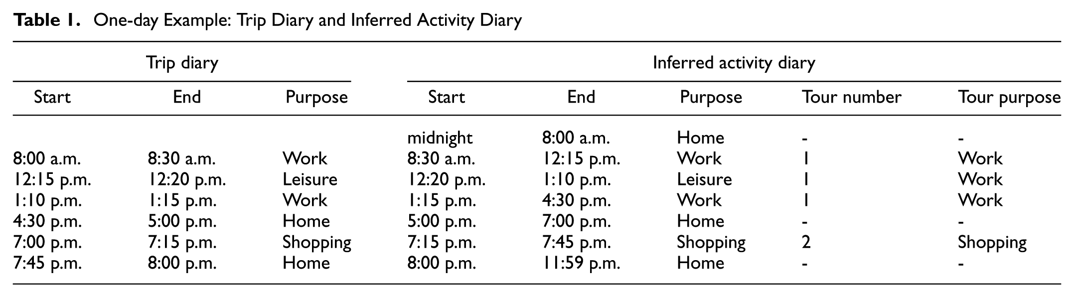
To facilitate the use of the chosen distance measures, the information about activity schedules was reduced to one main activity purpose per day. This main activity purpose was based on the construct of tours. Each day was divided into tours that both start and end at home. For example, the sample day in Table 1 consists of two tours. The purpose of any given tour was identified by the longest activity of the tour (e.g., work, for the first tour on the sample day). The main activity purpose per day was then determined by the following rule: If a day contained a work or education tour—that is, a mandatory activity—then the main activity purpose of that day would be work or education, respectively. Otherwise, the main activity purpose of the day was given by the purpose of the longest tour of that day. More information about the construction of activity schedules and the transformation process can be found in Hilgert et al. ( 22 ).

The reduction to one main purpose per day is a strict simplification of the activity patterns. It does not consider other aspects, such as tour concatenation, timing, or other activities during the week. When initially discussing this research idea, an appropriate dimension was sought for comparing activity patterns. Investigating all activities for the entire week would require analyzing patterns of different lengths. This, in turn, would require the application of different methods and increase the interpretation complexity. Moreover, there might be some activities during the week that are less important for the year-to-year comparison and the assessment of behavioral changes. In the end, the simplification described above was chosen to reduce the complexity of the approach and to allow the use of unidimensional methods (see next sections) that are more practical to handle and straightforward to interpret.

Distance Measures

As evidenced in the literature review, many different methods have been applied to investigate stability in travel behavior between two points of time. The level of stability depends strongly on the chosen measurement type and the number of attributes the measurement covers ( 3 ). With an increasing number of measurement attributes, the similarity of the strings usually decreases. Complex methods, such as multidimensional sequence alignment, are not useful for all research questions, because of the sharp increases in interpretation complexity. However, they are suitable for long, multidimensional sequences. When studying simple, short sequences, approaches such as the Hamming distance are also appropriate. Several studies in travel behavior apply these methods (partly as adapted versions) to compare strings ( 3 , 10 , 14 , 23 ). Here, two methods were chosen that permit straightforward interpretation and are appropriate for the research question. Using these methods, the frequencies and order of activities taking place within a week are compared.

Pairwise Edit Distance

The first distance measure implemented compares the corresponding days of two weeks from two different years. Here, weekly activity schedules were reduced to the information about main activity purposes. These, were called activity patterns. Then, each day of the first year was compared, pairwise, with the corresponding day of the second year. This distance is also known as the Hamming distance ( 7 ). The comparison is based on the days of the week (e.g., Monday in year 1 and Monday in year 2). If a given day has a different main activity purpose than in the previous year, a value of 1 is added to the distance. Thus, the maximum of this measure is 7 (all days have different purposes) and the minimum is 0 (all days have the same purposes) and the result can only be an integer. The Pairwise Edit Distance (PED) is calculated as

PED = \sum_{i = 1}^{7} d (i)

d (i) = {\begin{matrix} 0, & {MAP}_{i, 1} = {MAP}_{i, 2} \\ 1, & {MAP}_{i, 1} < > {MAP}_{i, 2} \end{matrix}

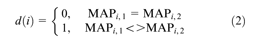
where

i = weekday number,

${MAP}_{i, 1}$ = main activity purpose of day i in year 1, and

${MAP}_{i, 2}$ = main activity purpose of day i in year 2.

Main Activity Distance

The second distance measure implemented also compares the main activity purposes of each day between different years. Unlike the PED, however, it does not take into account the sequence of the days. Instead, this measure compares the number of days for each activity purpose and counts differences between the two weeks. Differences in the purposes work, education, and home are weighted with 1.5; other purposes are weighted with 1. This weighting emphasizes the importance of mandatory activities, such as work and education. Home was also weighted with 1.5 to indicate whether a person stayed at home or undertook an activity on a given day. This results in a maximum of 21 for this measure (e.g., 7 working days in year one and 7 home days in year two) and a minimum of 0 (i.e., the distribution of activity purposes remains unchanged from year one to year two); only .0 and .5 values are feasible. The Main Activity Distance (MAD) is calculated as

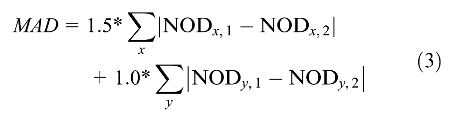
M A D = 1.5 * \sum_{x} | {NOD}_{x, 1} - {NOD}_{x, 2} | + 1.0 * \sum_{y} | {NOD}_{y, 1} - {NOD}_{y, 2} |

for $x \in {work, education, home}$ and $y \in {leisure, shopping, transport}$

where

${NOD}_{purpose, 1}$ = number of days with activity purpose in year 1, and

${NOD}_{purpose, 2}$ = number of days with activity purpose in year 2.

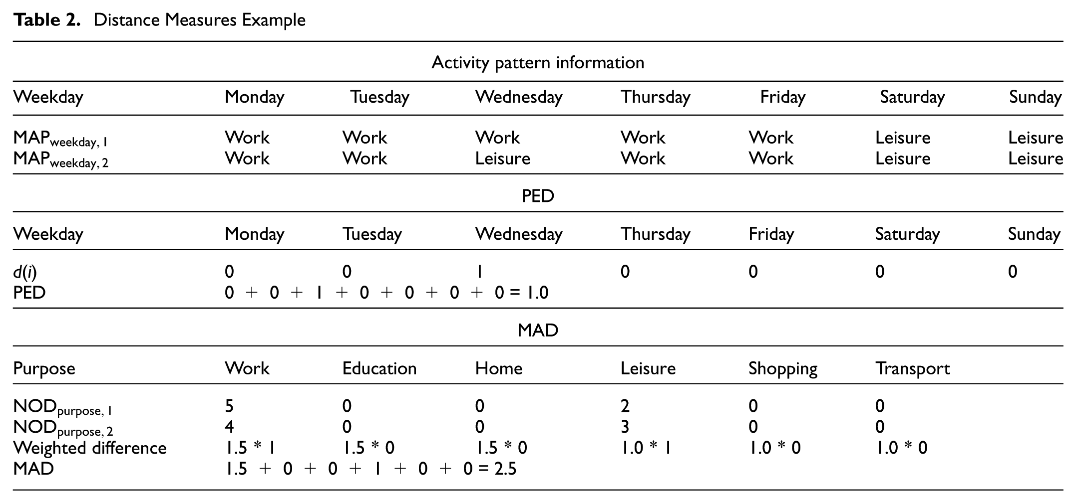
Distance Measures Example

To illustrate the differences between the distance measures, the following example is offered (see Table 2). Here, the individual worked from Monday to Friday in the first year. The weekend was dominated by leisure activities. In the second year, Wednesday was also dominated by leisure activities. Counting the number of different days (PED) yields 1. Counting the number of days per purpose (MAD) yields 2.5, since the “missing” working day is weighted by 1.5.

Table 2.

Distance Measures Example

Activity pattern information
Weekday	Monday	Tuesday	Wednesday	Thursday	Friday	Saturday	Sunday
${MAP}_{weekday, 1}$	Work	Work	Work	Work	Work	Leisure	Leisure
${MAP}_{weekday, 2}$	Work	Work	Leisure	Work	Work	Leisure	Leisure
PED
Weekday	Monday	Tuesday	Wednesday	Thursday	Friday	Saturday	Sunday
d(i)	0	0	1	0	0	0	0
PED	0 + 0 + 1 + 0 + 0 + 0 + 0 = 1.0
MAD
Purpose	Work	Education	Home	Leisure	Shopping	Transport
${NOD}_{purpose, 1}$	5	0	0	2	0	0
${NOD}_{purpose, 2}$	4	0	0	3	0	0
Weighted difference	1.5 * 1	1.5 * 0	1.5 * 0	1.0 * 1	1.0 * 0	1.0 * 0
MAD	1.5 + 0 + 0 + 1 + 0 + 0 = 2.5

Grouping Participants

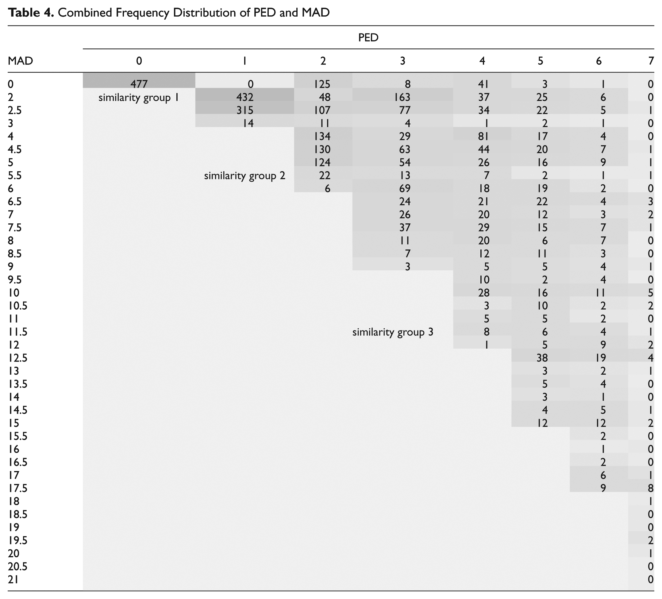
To evaluate differences between years, the PED and the MAD measures were combined to cluster participants into groups. Different groups of participants were tested in conjunction with the logistic regression model. Finally, participants were distinguished primarily according to the number of different days between the years (PED). Persons exhibiting larger differences were then further distinguished using the MAD measure. In the end, three groups of participants were defined according to their activity patterns:

PED <= 1: Participants having no or only small differences in their activity patterns.

n = 1,238 observations (35.5%)

PED > 1 AND MAD <= 6: Participants having bigger differences in their activity patterns but only small differences concerning the activity types over the whole week.

n = 1,642 observations (47.0%)

PED > 1 AND MAD > 6: Participants having bigger differences in their activity patterns and big differences concerning the activity types over the whole week.

n = 611 observations (17.5%)

Logistic Regression Model

To determine the relevant parameters that influence whether activity patterns between two years remain stable or not, a logistic regression model was used. Incorporating different variables into the model, tests were run to see which variables best predicted the “choice” of grouping. Thus, the model revealed parameters relevant for stable or instable behavior, as given by the distance measures PED and MAD. For the model, two different types of variables were used. The first type describes the participants’ situation in the second year (state variables). These variables include the socio-demographic characteristics (e.g., education level, household income, employment status) and the availability of mobility options (e.g., a car). The second type indicates differences between the years (change variables). For each transition between two years, it was determined whether variables such as education level or household income had changed. These changes were indicated using binary variables. If the variable had an ordinal scale, the size of the change would also be investigated. For the regression model estimate, the software tool SAS was used and the grouping of the participants as the dependent variable. Participant Group 1 was used as reference category.

Results

This section first describes the patterns for different population groups, which should deliver a first impression of relevant combinations among different people. It also shows the results of the implemented measures (PED and MAD) in a cross-table. Different state and change variables are then investigated and, finally, the results of the logistic regression model are shown.

Activity Patterns

To gain a better understanding of how often the various activity patterns (i.e., seven-digit chains of main daily activities during one week) occur among the different population groups, their frequency was compiled as a function of employment status (see Table 3). For each status, the five most common activity patterns are shown. Patterns occurring more rarely are summarized as “other.”

Table 3.

Activity Patterns by Frequency and Employment Status

Full-time workers		Part-time workers		Workers in vocational programs
Activity pattern	Frequency	Activity pattern	Frequency	Activity pattern	Frequency
WWWWWLL	31.8%	WWWWWLL	14.7%	EEEEELL	24.0%
WWWWWSL	15.4%	WWWWWSL	7.4%	WWWWWLL	8.3%
WWWWWWL	6.1%	WWWWWWL	3.0%	EEEEESL	7.4%
WWWWWWW	2.2%	WWWWWWW	2.3%	EEEEELH	2.8%
WWWWWLH	2.2%	WWWWLLL	2.0%	WWWWLLL	2.8%
Other	42.3%	other	70.6%	other	54.7%
Students at school or university		Pensioners
Activity pattern	Frequency	Activity pattern	Frequency
EEEEELL	44.4%	LLLLLLL	8.8%
EEEEESL	8.0%	LSLLLLL	2.7%
EEEEELH	4.7%	LLLLLSL	2.6%
EEEELLL	2.3%	LLLLSLL	2.6%
EEEEEHL	2.2%	SLLLLLL	2.4%
Other	38.4%	other	81.0%

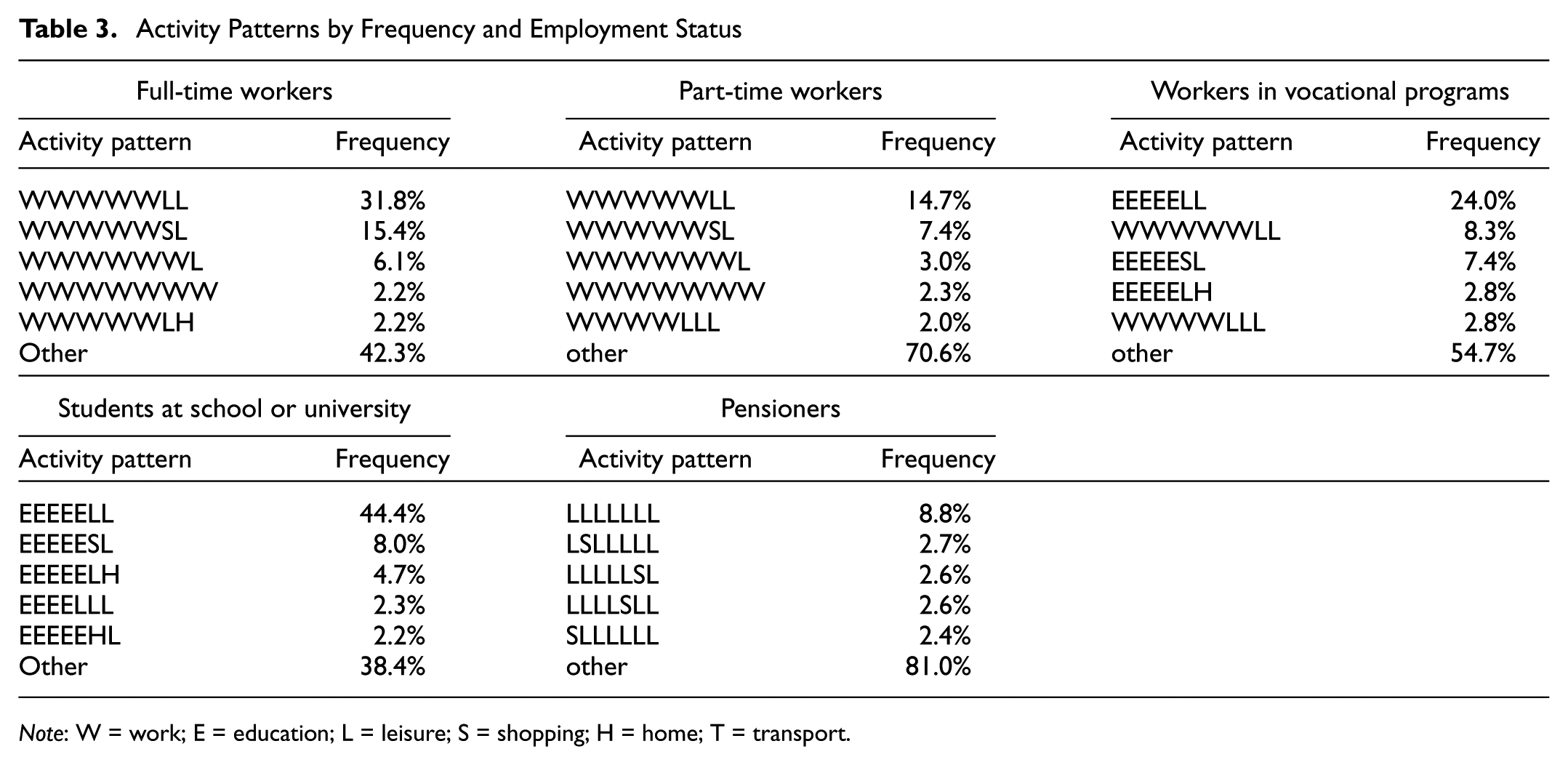
Note: W = work; E = education; L = leisure; S = shopping; H = home; T = transport.

Most activity patterns during weekdays (i.e., the first five digits of the chains) were characterized by obligatory activities, such as work or school. The most frequent activity pattern of both full-time and part-time workers was WWWWWLL. That is, Monday to Friday the main activities were working, whereas leisure activities dominated Saturday and Sunday. This activity pattern was more common for full-time workers (31.8%) than for part-time workers (14.7%), which suggests that the activity patterns of full-time workers are more homogeneous than those of part-time workers.

The most common activity pattern of workers in vocational programs (24.0%) and students (44.4%) was EEEEELL. In Germany, vocational education consists of two parts: theory learned in public vocational schools (activity purpose: education) and training embedded in a real-life work environment (activity purpose: work) ( 24 ). This dual scheme is evidenced by this group’s second most frequent activity pattern: WWWWWLL. For workers and students, leisure activities only dominated on the weekend. In contrast, the most frequent activity pattern of pensioners was LLLLLLL (8.8%), indicating that leisure was also likely to be the main activity on weekdays.

The highest share of “other” activity patterns (81.0%) among pensioners shows that their seven-day activity chains were more flexible than those of other employment groups. However, one must also take into consideration that pensioners generally had fewer activities than other groups ( 21 ). The activities they performed (e.g., shopping, leisure) were less often subject to weekly rhythms and their patterns were less often determined by mandatory activities. The lowest shares of “other” activity patterns were found among full-time workers (42.3%) and students (38.4%), a result that indicates a higher similarity in the activity patterns for members of these two groups and that might be expected, given the constraints of their work and study obligations.

Distance Measures

To illustrate the linkage of the similarity measures PED and MAD, Table 4 shows a combined frequency distribution. In total, 477 persons (13.7% of the sample) have results of 0 for both measures. In other words, their activity patterns were identical in the two years examined. If the main activities differ on only one day (e.g., WWWWWLL in year 1 and WWWWWSL in year 2), this person is still assigned to similarity group 1. The PED results for members of similarity group 2 (47.0% of the sample) and 3 (17.5%) range from 2 to 7. In other words, the main activities of at least two days differ from one year to the next. Similarity groups 2 and 3 are further distinguished using MAD. Group 2 contains people with lower MAD values (0 to 6) and group 3, people with higher MAD values (>6). Low MAD values (group 2) indicate similar frequencies for the main activity types. Here, it may be that the main activity types are merely allocated to different days of the week. The PED–MAD combination 3–2 is most common in similarity group 2, with 163 cases. One example of this activity pattern combination is WWWSWLL and WWSWWSL. Here, one leisure day is changed to a shopping day and the activity types of Wednesday and Thursday are switched. Since group 3 contains people with MAD values greater than 6, there are also larger differences in activity frequencies. There are 38 cases (6.2%) with the PED–MAD combination 5–12.5, as exemplified by the activity pattern combination WWWWWLL and LLLSSLL.

Table 4.

Combined Frequency Distribution of PED and MAD

MAD	PED
MAD	0	1	2	3	4	5	6	7
0	477	0	125	8	41	3	1	0
2	Similarity group 1	432	48	163	37	25	6	0
2.5	Similarity group 1	315	107	77	34	22	5	1
3		14	11	4	1	2	1	0
4			134	29	81	17	4	0
4.5			130	63	44	20	7	1
5			124	54	26	16	9	1
5.5		Similarity group 2	22	13	7	2	1	1
6		Similarity group 2	6	69	18	19	2	0
6.5				24	21	22	4	3
7				26	20	12	3	2
7.5				37	29	15	7	1
8				11	20	6	7	0
8.5				7	12	11	3	0
9				3	5	5	4	1
9.5					10	2	4	0
10					28	16	11	5
10.5					3	10	2	2
11					5	5	2	0
11.5				Similarity group 3	8	6	4	1
12				Similarity group 3	1	5	9	2
12.5						38	19	4
13						3	2	1
13.5						5	4	0
14						3	1	0
14.5						4	5	1
15						12	12	2
15.5							2	0
16							1	0
16.5							2	0
17							6	1
17.5							9	8
18								1
18.5								0
19								0
19.5								2
20								1
20.5								0
21								0

State Variables

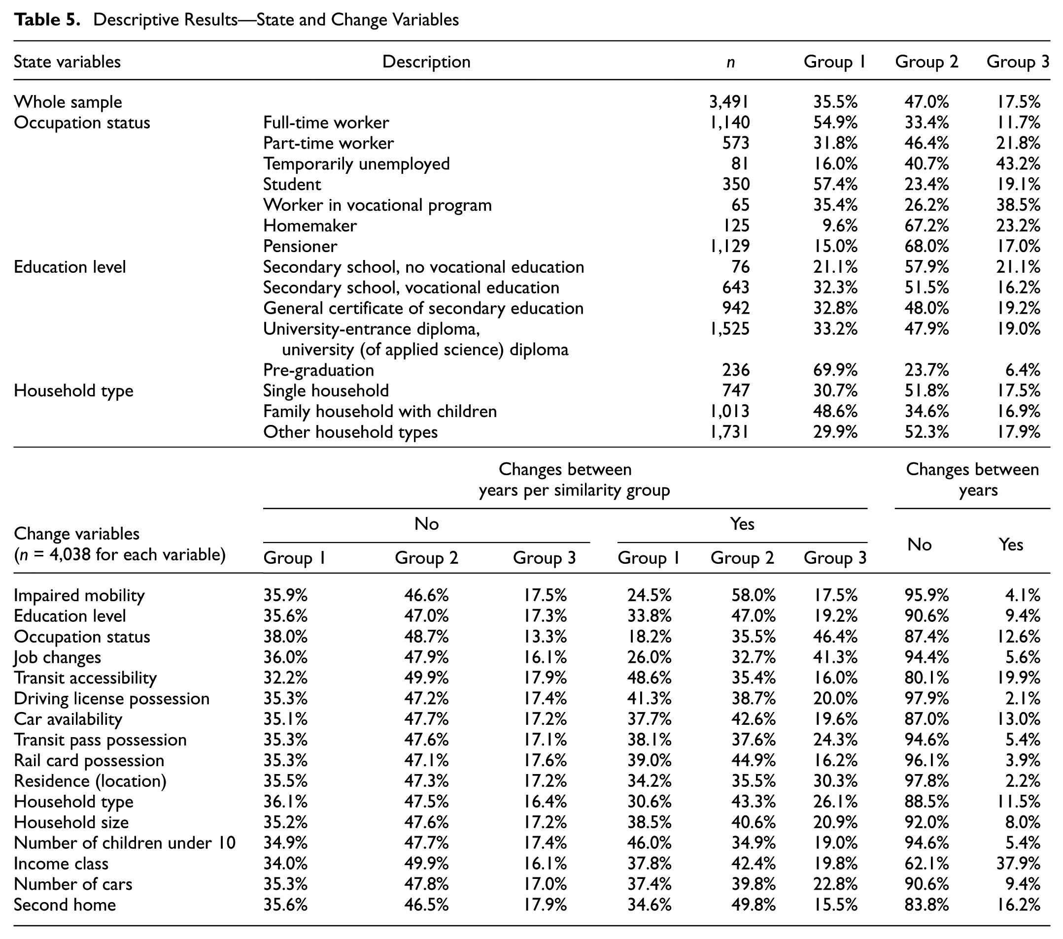
Variables of MOP data were categorized into state and change variables (see Table 5). State variables describe the participant in the second year, whereas change variables characterize a change between two years. Table 5 shows three state variables—occupation status, education level, and household type—along with their characteristic values, which sum to 100%. A majority (54.9%) of full-time workers landed in similarity group 1. Only students were more stable (57.4% in group 1). Part-time workers exhibited greater variability, with a plurality (46.4%) landing in similarity group 2. A plurality of temporarily unemployed persons and workers in vocational programs landed in similarity group 3. Persons with a pre-graduation education level—most of them are students in school—exhibited high stability, with almost 70% in group 1. Persons with secondary school and no vocational training had a higher percentage in group 2 (57.9%) than persons with other education levels. Single households were mostly in similarity group 2 and family households were to a large part in similarity group 1. Regarding their main activities, family households presumably exhibited more stable behavior than single households because of the more systematic routines needed to organize children households.

Table 5.

Descriptive Results—State and Change Variables

State variables	Description				n	Group 1	Group 2	Group 3
Whole sample					3,491	35.5%	47.0%	17.5%
Occupation status	Full-time worker				1,140	54.9%	33.4%	11.7%
	Part-time worker				573	31.8%	46.4%	21.8%
	Temporarily unemployed				81	16.0%	40.7%	43.2%
	Student				350	57.4%	23.4%	19.1%
	Worker in vocational program				65	35.4%	26.2%	38.5%
	Homemaker				125	9.6%	67.2%	23.2%
	Pensioner				1,129	15.0%	68.0%	17.0%
Education level	Secondary school, no vocational education				76	21.1%	57.9%	21.1%
	Secondary school, vocational education				643	32.3%	51.5%	16.2%
	General certificate of secondary education				942	32.8%	48.0%	19.2%
	University-entrance diploma, university (of applied science) diploma				1,525	33.2%	47.9%	19.0%
	Pre-graduation				236	69.9%	23.7%	6.4%
Household type	Single household				747	30.7%	51.8%	17.5%
	Family household with children				1,013	48.6%	34.6%	16.9%
	Other household types				1,731	29.9%	52.3%	17.9%
	Changes between years per similarity group						Changes between years
	No			Yes
Change variables(n = 4,038 for each variable)	Group 1	Group 2	Group 3	Group 1	Group 2	Group 3	No	Yes
Impaired mobility	35.9%	46.6%	17.5%	24.5%	58.0%	17.5%	95.9%	4.1%
Education level	35.6%	47.0%	17.3%	33.8%	47.0%	19.2%	90.6%	9.4%
Occupation status	38.0%	48.7%	13.3%	18.2%	35.5%	46.4%	87.4%	12.6%
Job changes	36.0%	47.9%	16.1%	26.0%	32.7%	41.3%	94.4%	5.6%
Transit accessibility	32.2%	49.9%	17.9%	48.6%	35.4%	16.0%	80.1%	19.9%
Driving license possession	35.3%	47.2%	17.4%	41.3%	38.7%	20.0%	97.9%	2.1%
Car availability	35.1%	47.7%	17.2%	37.7%	42.6%	19.6%	87.0%	13.0%
Transit pass possession	35.3%	47.6%	17.1%	38.1%	37.6%	24.3%	94.6%	5.4%
Rail card possession	35.3%	47.1%	17.6%	39.0%	44.9%	16.2%	96.1%	3.9%
Residence (location)	35.5%	47.3%	17.2%	34.2%	35.5%	30.3%	97.8%	2.2%
Household type	36.1%	47.5%	16.4%	30.6%	43.3%	26.1%	88.5%	11.5%
Household size	35.2%	47.6%	17.2%	38.5%	40.6%	20.9%	92.0%	8.0%
Number of children under 10	34.9%	47.7%	17.4%	46.0%	34.9%	19.0%	94.6%	5.4%
Income class	34.0%	49.9%	16.1%	37.8%	42.4%	19.8%	62.1%	37.9%
Number of cars	35.3%	47.8%	17.0%	37.4%	39.8%	22.8%	90.6%	9.4%
Second home	35.6%	46.5%	17.9%	34.6%	49.8%	15.5%	83.8%	16.2%

Change Variables

The change variables in Table 5 describe a possible change (e.g., of occupation status) between the two years. The frequency of these changes occurring among all individuals in the sample and for each similarity group are displayed. The impaired mobility variable signifies changes in physical mobility from one year to the next. Here, only a few changes (4.1%) are recorded in the sample. People whose physical mobility does change are most likely to be in similarity group 2 (58.0%). More changes are visible in the education level variable, which indicates a graduation event between the first and second years. In 9.4% of the sample, there was a change in education level, and most of these people are found in similarity group 2. A change in occupation status makes it more likely for people to be in similarity group 3, showing the important influence of this variable. In 19.9% of survey participants, there was a change in transit accessibility (i.e., the accessibility of work place or school by public transit). This might be correlated with changes in job, occupation, or residence location. Most people with transit accessibility changes still belong to similarity group 1, implying that such a change does not lead to significantly altered activity patterns. Changes in residence or in the possession of driving license, transit pass, or rail card take place relatively seldom (in each case, less than 6% of the sample). There were many shifts in income class in the sample (37.9%). Most of these shifts were in similarity groups 1 and 2. Changes in household type are also considered in the analysis (e.g., changing to a family household when a child arrives through birth or adoption). The variable household size captured changes in the number of people in the household. The second home variable was included, since it might also explain why travel patterns change from year to year. In 16.2% of the sample, there were changes in second home ownership, and most of these people belonged to similarity group 2.

Logistic Regression Model

The logistic regression model helps illustrate how various socio-demographic characteristics influence the probability of a person belonging to one of the three similarity groups. Table 6 shows estimates and significance levels for the parameters included in the model. All socio-demographic characteristics (state and change variables) have been defined as binary variables. The reference category was similarity group 1.

Table 6.

Results—Logistic Regression

No.	Variable	Wald chi-square	Parameter estimates
No.	Variable	Wald chi-square	Similarity group 2	Similarity group 3
0	Intercept		1.364***	−0.198*
1	person is full-time worker	354.339***	−1.94***	−1.712***
2	person is part-time worker	62.256***	−1.026***	−0.746***
3	person is student	165.301***	−2.134***	−0.956***
4	person is worker in vocational program	27.652***	−1.766***	−0.814**
5	person holds a general qualification for university entrance, high school, or university degree	15.766***	0.278***	0.387***
6	person lives in family household with children	8.359**	−0.266***	−0.251**
7	occupation status has changed	213.634***	0.286*	1.837***

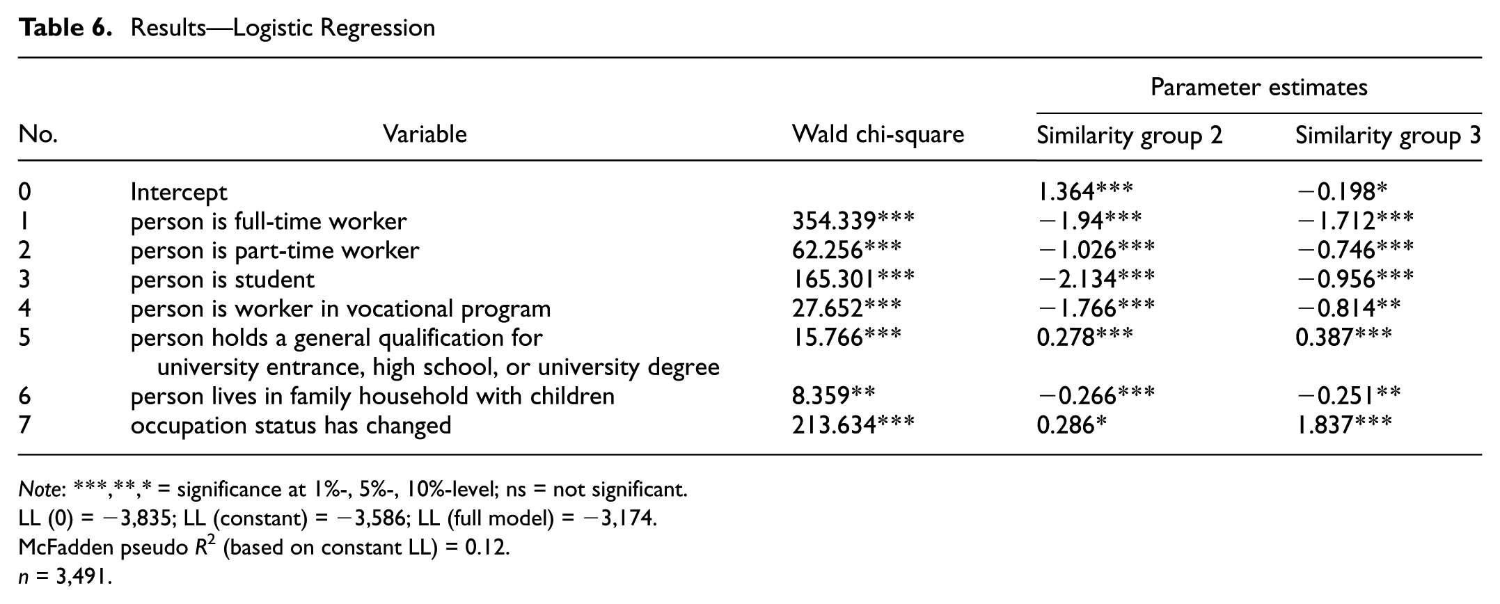
Note: ***,**,* = significance at 1%-, 5%-, 10%-level; ns = not significant.

LL (0) = −3,835; LL (constant) = −3,586; LL (full model) = −3,174.

McFadden pseudo R² (based on constant LL) = 0.12.

n = 3,491.

The Wald Chi Square results show that all variables included in the regression model were significant. The values of the Wald Chi Square results indicate that occupation has the highest explanatory power for both the state (occupation status) and change (change of occupation status) variables. For the occupation state variables, the reference consists of all people without employment, that is, pensioners, unemployed people, and homemakers. People of all occupation groups (variables 1 to 4) are less likely to be in similarity group 2 or 3 than in the reference category, since all estimates are negative. Survey participants with higher education levels tended to be more flexible than those with lower education levels. Possibly, they had more activity options on the weekend, resulting in both higher PED and higher MAD values. Interestingly, households with children were more stable than the reference households (households with 2+ adults but no children; single-households). Living with children typically requires more plans and agreements in everyday life, and once these routines have been established, families might be reluctant to give them up.

Considering the change variables, it was seen that a change in occupation status, such as moving from education to full-time work or from full-time work to retirement, explained differences in similarity groups quite well. Participants with a change in occupation status were more likely to be in group 3, since a new status is often associated with different activities. These results are in line with the descriptive findings.

The other change and state variables tested such as car ownership, spatial type, income, gender, the existence of children in the household (category 1), change of residence, employment status, and household size turned out not be significant in the regression model.

Conclusions

Routines and mandatory activities, such as working, determine individual activity patterns and strongly influence travel demand. However, the variability or stability in people’s activity patterns from one year to the next has not been previously researched. Knowledge about the year-to-year stability of activity patterns and information about how changes in life circumstances affect this stability can make an important contribution to rational transport policies and facilitate the modeling and forecasting of travel demand.

To analyze activity patterns, two distance measures were used—PED and MAD. These measures compare weekly activity patterns. The activity information for a given week was distilled down to the main activity purposes for each day of that week. Using survey responses from the MOP, those participants who had responded multiple times and evaluated their activity pattern changes between two successive years of participation were selected for the sample. First the activity patterns were analyzed descriptively. About one-third of the sample participants had the same or very similar main activity patterns in the two weeks examined. The group identified as workers had the highest propensity of similar activity patterns. Around 50% had patterns consisting of five days of work and two days dominated by leisure and shopping. Pensioners, in contrast, had more flexible activity patterns. Since their behavior is not so restricted by mandatory activities, such as working or attending school, a wider variety of activity patterns becomes possible. Results reveal the variable “occupation status” (e.g., worker, student or pensioner) to be the most important for describing similarity groups. About 55.1% of full-time workers were in similarity group 1, but only 14.3% of pensioners. In addition, the change variable “occupation status has changed” had a high explanatory power for activity pattern variability: people whose occupation status changed were more likely to belong to similarity group 2 or 3.

Nevertheless, the study has several limitations. First, the definition of similarity groups is very subjective. Since the degree of freedom in defining a similarity group is very high, future research should explore how changing this definition affects the results. Second, the small number of observations involving life events might have obscured the significance of change variables in the logistic regression. An extension of the data with new survey waves would improve the levels of significance. Third, further research is needed on the definition of activity patterns for year-to-year comparison. Here, only the main daily activities for the study week were considered. A refinement of the approach would be to consider all activities during the week. However, this would expand the complexity of the activity patterns and possibly require the use of other distance measures. Another interesting project would be to combine activity pattern measures with land use aspects or mode choice decisions, an endeavor that would also tend to increase the complexity of the analysis.

Footnotes

Acknowledgements

This publication was written within the framework of the Profilregion Mobilitätssysteme Karlsruhe, which is funded by the Ministry of Science, Research and the Arts in Baden-Württemberg.

Author Contributions

The authors confirm contribution to the paper as follows: study conception and design: T. Hilgert, S. von Behren, C. Eisenmann, P. Vortisch; data collection: T. Hilgert, S. von Behren, C. Eisenmann; analysis and interpretation of results: T. Hilgert, S. von Behren, C. Eisenmann, P. Vortisch; draft manuscript preparation: T. Hilgert. All authors reviewed the results and approved the final version of the manuscript.

The Standing Committee on Traveler Behavior and Values (ADB10) peer-reviewed this paper (18-01379).

References

Cherchi

Cirillo

Understanding Variability, Habit and the Effect of Long Period Activity Plan in Modal Choices: A Day to Day, Week to Week Analysis on Panel Data. Transportation, Vol. 41, 2014, pp. 1245–1262.

Raux

T.-Y.

Cornelis

Variability in Daily Activity-travel Patterns: The Case of a One-week Travel Diary. European Transport Research Review, Vol. 8, No. 4, 2016, p. 26.

Schlich

. Analysing Intrapersonal Variability of Travel Behaviour Using the Sequence Alignment Method. Proc., AET European Transport Conference, Cambridge, UK, 2001. http://webarchiv.ethz.ch/ivt/vpl/publications/reports/ab80.pdf

Schönfelder

. Urban Rhythms - Modelling the Rhythms of Individual Travel Behaviour. PhD thesis. Institute of Transport Planning and Systems, Swiss Federal Institute of Technology, Zurich, 2006.

Bayarma

Kitamura

Susilo

Recurrence of Daily Travel Patterns: Stochastic Process Approach to Multiday Travel Behavior. Transportation Research Record: Journal of the Transportation Research Board, 2007. 2021: 55–63.

Buliung

R. N.

Roorda

M. J.

Remmel

T. K.

Exploring Spatial Variety in Patterns of Activity-travel Behaviour: Initial Results from the Toronto Travel-Activity Panel Survey (TTAPS). Transportation, Vol. 35, No. 6, 2008, pp. 697–722.

Hamming

R. W.

Error Detecting and Error Correcting Codes. Bell System Technical Journal, Vol. 29, No. 2, 1950, pp. 147–160.

Hosangadi

Distance Measures for Sequences, 2012, pp. 1–16.

Joh

C.-H.

Arentze

T. A.

Timmermans

H. J. P.

Multidimensional Sequence Alignment Methods for Activity-Travel Pattern Analysis. A Comparison of Dynamic Programming and Genetic Algorithms. Geographical Analysis, Vol. 33, No. 3, 2001, pp. 247–270.

10.

Bargeman

Joh

C.-H.

Timmermans

Vacation Behavior Using a Sequence Alignment Method. Annals of Tourism Research, Vol. 29, No. 2, 2002, pp. 320–337.

11.

Wilson

Analysis of Travel Behavior Using Sequence Alignment Methods. Transportation Research Record: Journal of the Transportation Research Board, 1998. 1645: 52–59.

12.

Saneinejad

Roorda

Application of Sequence Alignment Methods in Clustering and Analysis of Routine Weekly Activity Schedules. Transportation Letters: The International Journal of Transportation Research, Vol. 1, No. 3, 2009, pp. 197–211.

13.

Kwan

M.-P.

Xiao

Ding

Assessing Activity Pattern Similarity with Multidimensional Sequence Alignment based on a Multiobjective Optimization Evolutionary Algorithm. Geographical Analysis, Vol. 46, 2014, pp. 297–320.

14.

Joh

C.-H.

Arentze

Timmermans

Pattern Recognition in Complex Activity Travel Pattern : Comparison of Euclidean Distance, Signal-processing Theoretical, and Multidimensional Sequence Alignment Methods. Transportation Research Record: Journal of the Transportation Research Board, 2001. 1752: 16–22.

15.

Jones

Clarke

The Significance and Measurement of Variability in Travel Behaviour. Transportation, Vol. 15, 1988, pp. 65–87.

16.

Huff

J. O.

Hanson

Repetition and Variability in Urban Travel. Geographical Analysis, Vol. 18, No. 2, 1986, pp. 97–114.

17.

Hanson

Huff

O.J.

Systematic Variability in Repetitious Travel. Transportation, Vol. 15, 1988, pp. 111–135.

18.

Pas

E. I.

Koppelman

F. S.

An Examination of the Determinants of Day-to-day Variability in Individuals’ Urban Travel Behavior. Transportation, Vol. 14, 1987, pp. 3–20.

19.

Pas

E. I.

A Fexible and Integrated Methodology for Analytical Classififaction of Daily Travel-Activity Behavior. Transportation Science, Vol. 17, No. 4, pp. 405–429.

20.

Weiss

Chlond

Minster

Jödden

Vortisch

Assessing the Effects of a Mixed-Mode Design in a Longitudinal Household Travel Survey. Presented at 96th Annual Meeting of the Transportation Research Board, Washington, D.C., 2017.

21.

Weiss

Chlond

von Behren

Hilgert

Vortisch

Deutsches Mobilitätspanel (MOP) - Wissenschaftliche Begleitung und Auswertungen Bericht 2015/2016: Alltagsmobilität und Fahrleistung [German Mobility Panel - Scientific Supervision and Analyses Report 2015/2016: Everyday Travel and Car Use], Karlsruhe, 2016.

22.

Hilgert

Heilig

Kagerbauer

Vortisch

Modeling Week Activity Schedules for Travel Demand Models. Transportation Research Record: Journal of the Transportation Research Board, 2017. 2666: 69–77.

23.

Streit

Allier

C.-E.

Weiss

Chlond

Vortisch

Changes in Variability and Flexibility of Individual Travel in Germany – Trends and Drivers. Presented at 94th Annual Meeting of the Transportation Research Board, Washington, D.C., 2015.

24.

Federal Ministry of Education and Research. The German Vocational Training System. https://www.bmbf.de/en/the-german-vocational-training-system-2129.html. Accessed July 13, 2017.