How Accurately Can We Measure from Video? Practical Considerations and Enhancements of the Camera Calibration Procedure

Abstract

The accuracy of position measurements from videos depends greatly on the quality of the camera calibration model parameters. This paper investigates how such factors as camera height and the selection of calibration points affect the quality of the final calibration model. A series of controlled experiments were performed in traffic or similar-to-traffic environments, in which the accuracy of measurements from videos was compared with measurements taken with other tools. To enhance the calibration process, a multi-camera approach is suggested that utilizes the information about “common points” – points seen on several cameras but with unknown world coordinates. The performed tests showed that calibration quality can greatly benefit from this approach. The paper is addressed primarily to traffic researchers developing their own video-based tools for road user observations.

The video recording and extraction of microscopic data, such as road user position and speed, from videos is a commonly used method in many road traffic studies. Examples of such applications include surrogate safety analysis ( 1 – 5 ), behavioral analysis ( 6 , 7 ), and the calibration of microscopic traffic models ( 8 – 10 ). 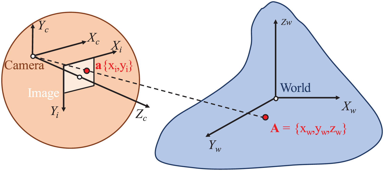A crucial step before objective measurements from a video can be taken is camera calibration, that is, the definition of a model that relates the position of a point A in world coordinates (x_w, y_w, z_w) to its representation a (x_i, y_i) in the camera image (Figure 1).

Figure 1.

Calibration model principle.

Several techniques for camera calibration have been suggested, the most common being Heikkilä and Silven, Tsai, and Zhang ( 11 – 13 ). This study uses the Tsai calibration model, which incorporates linear equations based on the radial alignment constraint and a second-order radial term that handles lens distortions (the exact mathematical description can be found elsewhere, e.g., Tsai [ 12 ]).

One important mathematical property of the calibration model deserves a mention here. Transforming three-dimensional (3D) world coordinates to an image can be done unambiguously, but this is not the case for transforming in the opposite direction (from an image to the world). An image point corresponds to a series of points in the 3D space or, more specifically, all the points along a ray (see the dashed line in Figure 1). Therefore, it is necessary to have additional information (usually, the point’s z-coordinate) to define a single corresponding point in the real world. This problem is often tackled using an approximation that states the part of the road surface visible in an image is a perfect plane, that is, the z-coordinate of the road user footprint is always zero (we will refer to this later as the “zero-plane”).

The parameters of the calibration model with a fixed mounted camera are usually estimated based on a set of points with a known position in an image and known world coordinates. Once again, we omit the heavy mathematical description of the process, which can be found, for example, in Tsai ( 12 ).

Video-based tools available on the market usually come with a list of recommendations on how the cameras should be installed ( 14 ). However, a traffic researcher willing to develop their own tools with functionality beyond what the “standard sensors” have to offer, usually has to find his/her own way by trial and error, which might often be costly in time, energy, and amount of frustration. The purpose of this paper is to provide practical hints and a better understanding about which factors affect the quality of the camera calibration model and consequently the measurements taken from a video and the extent of these effects. Several real-world experiments have been conducted testing the different factors, such as camera perspective, location of the points used for calibration, and so forth. A multi-camera approach is also suggested to enhance the quality of the calibration model.

In this study, we use used a software tool called T-Calibration ( 15 ), which is available as a free download. The software is based on Tsai’s model description ( 12 ) except for the module on model parameters’ initialization, which utilizes the code of Reg Willson ( 16 ).

What Affects the Accuracy of Measurements from a Video?

A long list of factors can affect the accuracy of measurements taken from a video. The most important are:

Camera height and perspective,

Camera resolution,

The distance from the camera to the studied object (see Figure 2),

The quality of the calibration model.

Figure 2.

The “size” of one camera image pixel in real-world distance units.

An objective measure of the calibration model quality is the discrepancy between the actual position of a calibration point in the image and the projection to the image of its world coordinates (further noted as e, measured in pixels) or, alternatively, the actual position of a calibration point in the world and its projection from the image (further noted as E, measured in meters) – see Figure 3. As the optimization criteria of the calibration model parameters, minimization of one of the following parameters can be used:

Ē, m – average of the discrepancies between the points in world coordinates and their projections from the camera view,

E_max, m – maximum discrepancy value in world coordinates,

ē, pxl – average of the discrepancies between the points and their projections from the world in the camera image,

e_max, pxl – maximum discrepancy value in the camera image.

Figure 3.

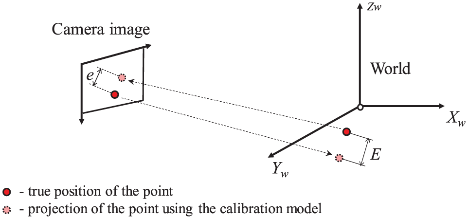
Discrepancies between the true and “projected” positions of a calibration point due to imperfections of the calibration model.

However, the final judgment of the obtained calibration model is as much an art as it is a precise science. Low values for E and e do not necessarily guarantee an accurate calibration model. In practice, the number of available calibration points is usually limited, and these points do not necessarily cover the entire scene as evenly as desired. In this case, the optimization may “force” the model to fit the available points well, but for the areas with no points, the calibration quality will remain uncertain.

At least some initial clues regarding the general model fit can be obtained from a visual check. This can be done by, for example, placing a grid of regularly positioned points in the road plane and projecting them to the camera view. Strange curvatures and distortions (Figure 4) would indicate that a further enhancement of the calibration model is necessary.

Figure 4.

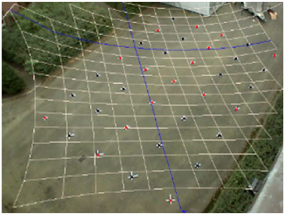
The grid placed on the road surface suggests the poor quality of the calibration model, even though the error metrics on the calibration points are low.

Dataset I

Data Collection Set-Up

A grid of 35 points (cell size 2 m) was marked on a flat, traffic-free space surrounded by building blocks (Figure 5). Cameras 1 and 2 were installed almost exactly above each other on the outdoor emergency ladder (heights 5.5 m and 8 m respectively) and cameras 3 and 4 on the roof (height 11 m). The points’ positions were measured accurately with a theodolite (measurement error <1 cm). The height difference between the individual points did not exceed 1 to 2 cm, and, despite being considered in all calculations, it did not produce any noticeable effect.

Figure 5.

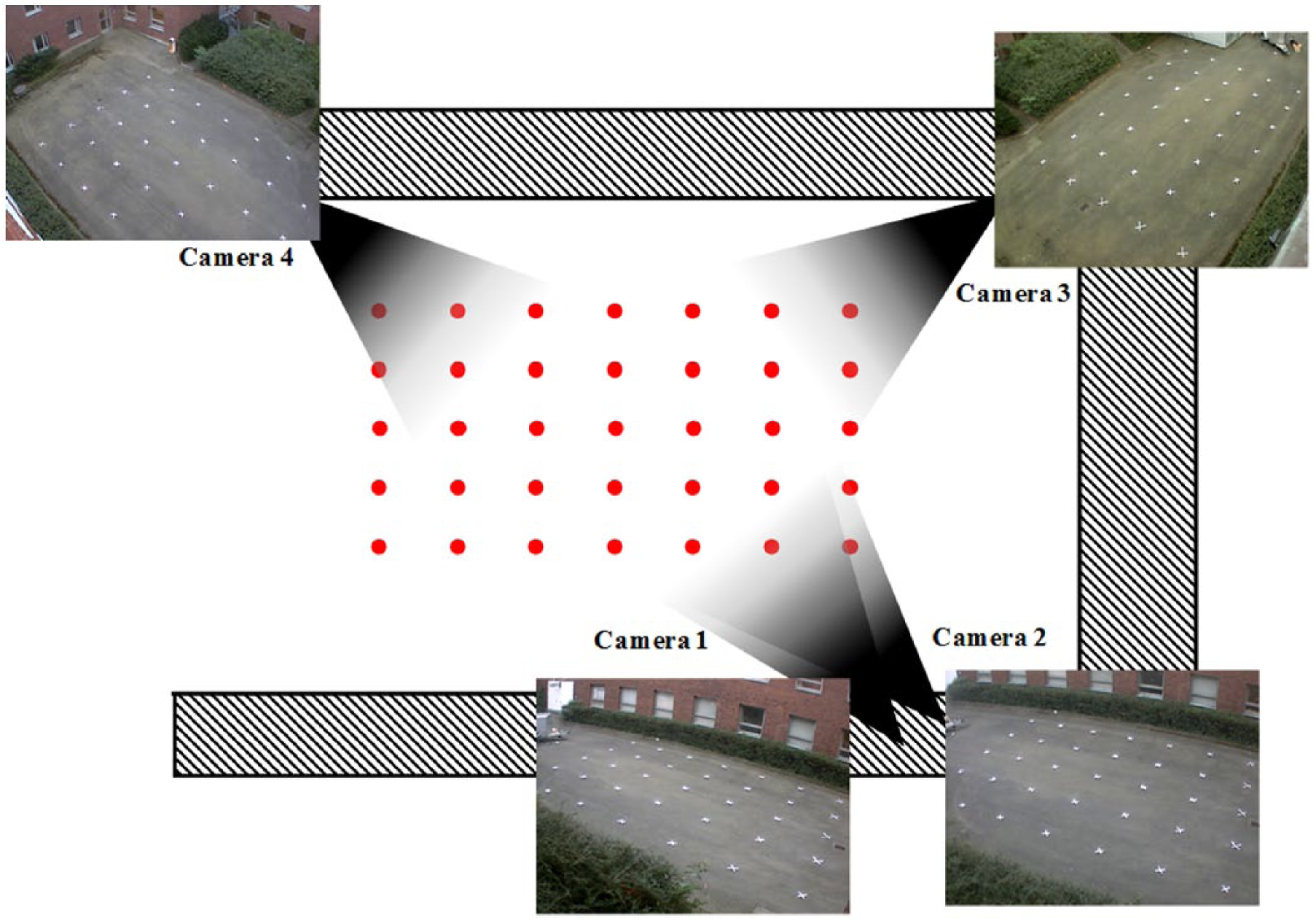
Camera set-up for Dataset I.

This set-up is much more accurate compared with what is considered “normal” accuracy in traffic studies. In a sense, it is a controlled simulation, close enough to real road environments, but it allows for testing of the effects of different factors, such as the selection of calibration points, camera angle, and introduced errors in calibration point coordinates.

Experiment 1

The main objective of this experiment was to investigate how the camera angle and the selection of calibration points affect the final calibration model quality. Views from cameras 1, 2, and 3 were used, as their views of the calibration points were highly similar (though “mirrored” for Camera 3), except for the camera installation heights. The following scenarios were tested (Figure 6):

S1 : all the available points used for calibration;

S2 : few points evenly distributed over the outer border of the studied area and no points in the middle; this is a typical situation for an urban intersection where many calibration points can be found at zebra crossings around the intersection, but there are no points in its central part;

S3 : few points concentrated in the corner close to the camera;

S4 : few points in the corner far away from the camera.

Figure 6.

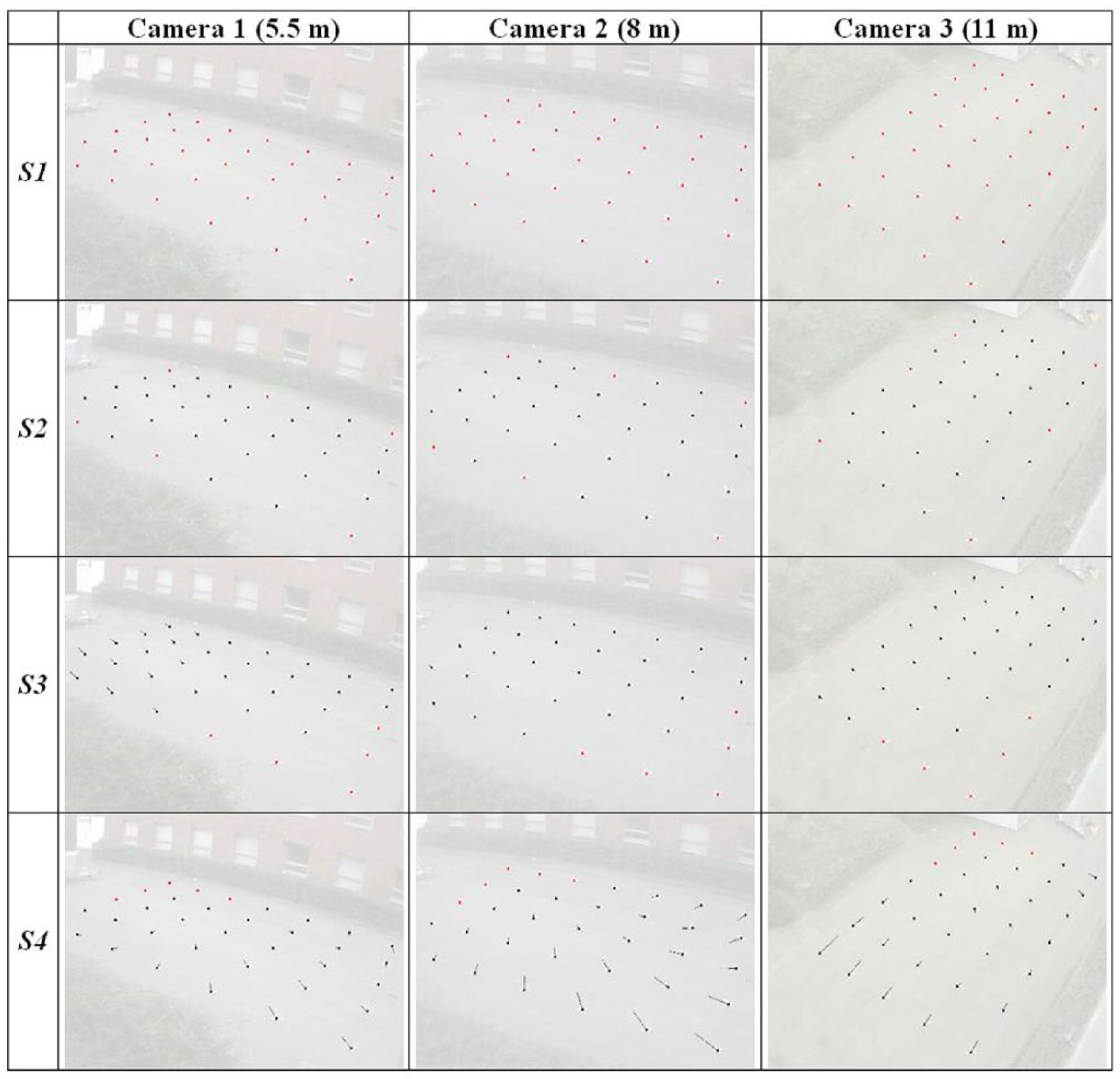
Calibration point selection for Experiment 1. Points used for calibration are marked red. Error vectors connect the points in the image with the projection of the corresponding point from the world coordinates. Note how error vectors increase with distance from the calibration points in scenarios S3 and S4.

The results are presented in Figure 6 and Table 1. Scenario S1 is the “perfect case,” in which many calibration points are evenly distributed over the entire image. All three camera installations provide excellent accuracy, even though it can be noted that, in full accordance with the basic rules of geometry, real-world errors slightly increase as the camera height lowers.

Table 1.

Calibration Quality Parameters for Experiment 1

		Camera 15.5 m	Camera 28 m	Camera 311 m
S1	Points	34	34	35
	Ē, cm	2	1	1
	E_max, cm	9	5	3
	ē, pxl	0	0	0
	e_max, pxl	1	1	1
S2	Points	6	6	6
	Ē, cm	3 (2)	2 (1)	3 (1)
	E_max, cm	10 (10)	5 (4)	8 (3)
	ē, pxl	1 (1)	1 (0)	1 (0)
	e_max, pxl	3 (1)	2 (2)	2 (1)
S3	Points	5	5	5
	Ē, cm	25 (1)	8 (0)	19 (1)
	E_max, cm	93 (5)	35 (1)	73 (2)
	ē, pxl	5 (0)	2 (0)	4 (0)
	e_max, pxl	19 (2)	5 (0)	9 (1)
S4	Points	5	5	5
	Ē, cm	24 (2)	42 (4)	31 (0)
	E_max, cm	87 (8)	92 (13)	149 (1)
	ē, pxl	8 (0)	15 (1)	10 (0)
	e_max, pxl	28 (1)	54 (2)	47 (0)

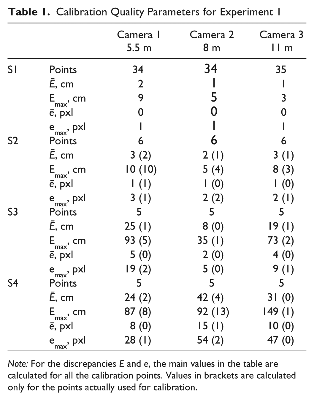
Note: For the discrepancies E and e, the main values in the table are calculated for all the calibration points. Values in brackets are calculated only for the points actually used for calibration.

Scenario S2, despite the increase in errors, still appears quite usable, as the points, though not as frequent as in S1, still cover a large area of the image. Adversely, scenarios S3 and S4 clearly demonstrate how the accuracy deteriorates as the measurements are attempted in the image areas that do not have any calibration points in the vicinity. A bit surprisingly (and against what theory would suggest), the increased camera height does result in systematically improved accuracy from Camera 1 to Camera 3 within these scenarios. It appears the location of the calibration points has a much stronger effect on the overall accuracy compared with what can be gained from the increased camera height.

Experiment 2

This experiment investigates how the accuracy of the world coordinates for the calibration points affects the calibration model’s quality. It is common that instead of measuring the points with a theodolite or similar high-accuracy instrument in the field, their positions are extracted from satellite photos provided by such services as Google Earth or Bing Maps. Such photos are often blurry and outdated, and even though they provide a good general overview and indicate approximately where the point should be, the actual position measured is not quite accurate.

In this test, we used the points from Scenario S2 in the previous experiment, as it is the most typical situation in the case of traffic videos. The actual world coordinates of the calibration points were modified with added errors dx and dy, generated randomly from a normal distribution with μ = 0 and chosen σ. The calibration procedure was repeated 100 times with newly generated dx and dy values. The final distributions of the calibration errors are presented in Figure 7.

Figure 7.

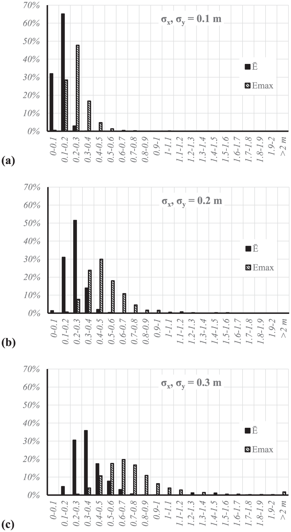
Distribution of the calibration Ē and E_max for simulated “inaccurate” world coordinates of the calibration points.

If the random variables that characterize the population are normally distributed, then there is approximately a 95% probability that the sample mean is within ±2 standard deviations of the population mean (i.e., it can be roughly assumed that σ = 10 cm represents the accuracy of the point measurement ±20 cm). It can be seen from Figure 7 that even with a small σ, there are some cases with an E_max value up to 80 cm, which is clearly unusable. This indicates how important it is to ensure that the obtained calibration model really makes sense, for example, using a visual check (Figure 4). “Guessing” the position of the points, which are not really seen in the satellite image, is probably not advisable either.

Experiment 3

In this test, we examined whether the use of a multi-camera set-up could improve the calibration quality of each individual camera. It is common that the potential calibration points clearly detectable in the satellite image are not visible in the camera view and vice versa. However, if several camera views are available, points not seen on one camera might be seen on another, and so forth. Moreover, there are usually many “common” points found in all camera views, but not in the satellite image. Examples of such points can include water traces on asphalt, shadows, or the wheel position of a stopped vehicle (given that the camera images are taken at approximately the same time).

The following algorithm for multi-camera calibration is suggested.

Each camera is calibrated independently based on “few” points that can be identified in both the satellite image and the camera view.

The “common” points are projected to the world coordinates using the available calibration models.

Because the world coordinates of a point suggested by each camera differ, they are “weighed” into a single value in the simplest case by taking an average.

Each camera is again calibrated, now using an extended set of points with world coordinates.

Steps 3 to 5 are repeated until further iterations do not yield any improvements.

To test this approach, we used the views from cameras 1 and 4. For the initial calibration, a highly limited and unfavorable set of points was selected (Figure 8). These were complemented by 10 common points marked in each camera but without the real-world coordinates. After approximately 10 iterations, no visible changes were produced. The results of the initial individual calibration and final multi-camera calibration are presented in Table 2.

Figure 8.

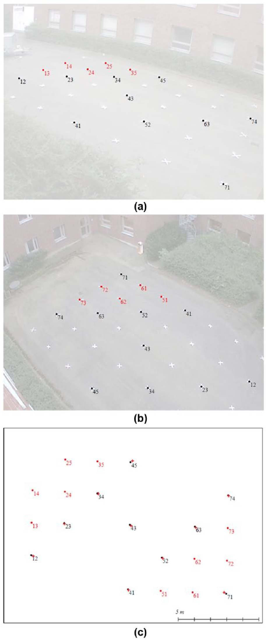
Multi-camera calibration: (a) Camera 1 view, (b) Camera 4 view, and (c) mapping of the calibration points in the real world. In red, the original points with known real-world positions; in black, the “common points” and their true real-world positions; red cross, the estimated positions of the common points in the real world.

Table 2.

Calibration Quality with Single- and Multi-Camera Approaches

	Individual calibrations		Multi-set-up calibrations
	Camera 1	Camera 4	Camera 1	Camera 4
Ē, cm	20	6	9	7
E_max, cm	66	25	24	14
ē, pxl	8	2	3	2
e_max, pxl	41	9	9	6

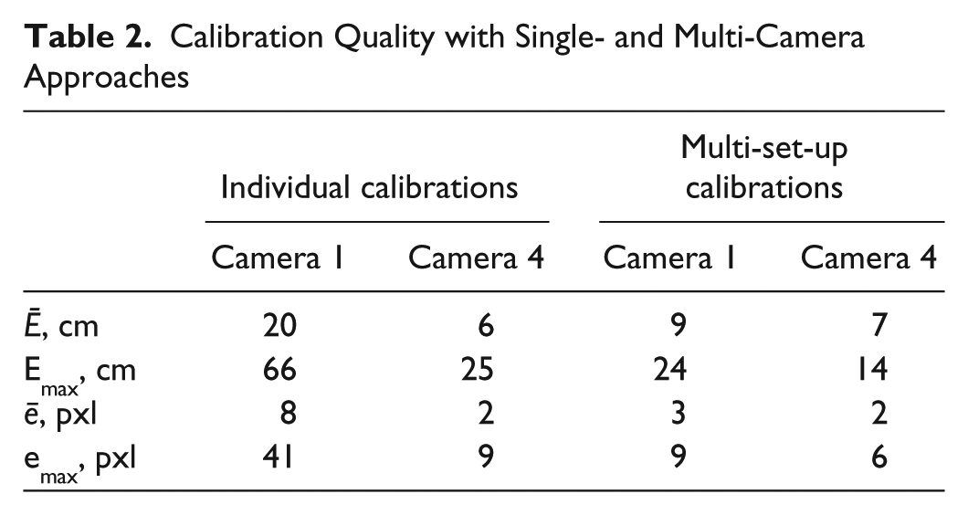
The use of additional calibration points, despite their estimated and not perfectly accurate real-world position, greatly improved the calibration accuracy, particularly for Camera 1, in which both the average and maximum errors greatly decreased. For Camera 4, the average error did not change, but the maximum error decreased, indicating the calibration became more consistent over the entire image.

Dataset II

Data Collection Set-Up

The second location was a real traffic intersection (Figure 9). It was filmed with a camera installed on the top of a water tower. An additional photo image was taken from a building on the opposite side of the intersection. The calibration points were limited to the actual landmarks, such as sharp corners of the road markings. The calibration point position was measured with a high-precision GNSS receiver (Leica GX1230 GG, http://www.leica-geosystems.com/), providing accuracy for static points of 1.5 to 2 cm. Most of the measured points could also be found in a satellite image from Googl Maps.

Figure 9.

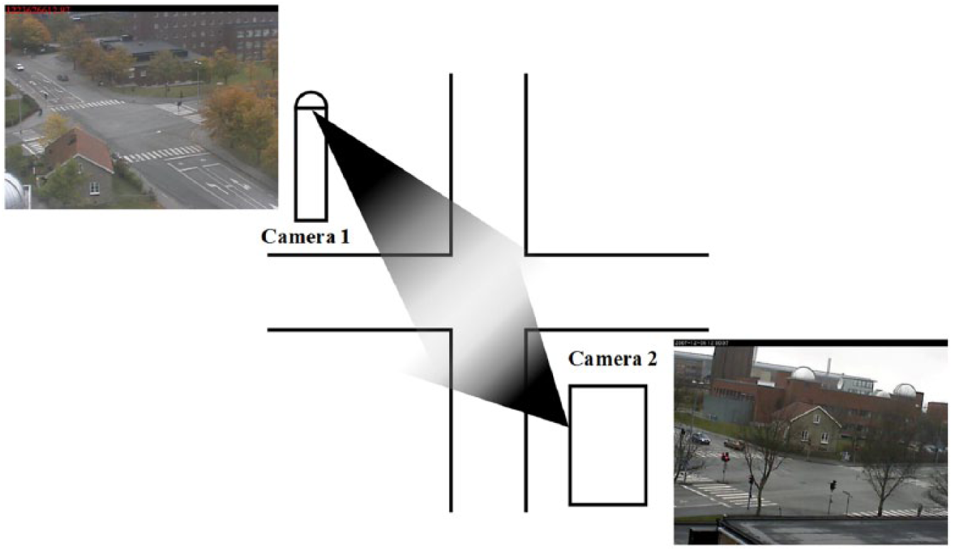
Camera set-up for Dataset II.

A car, equipped with the same type of GNSS receiver, drove through the intersection several times, performing different maneuvers. The position was saved with a frequency of 5 Hz; however, the accuracy of the measurement was affected by the movement and short time for each measurement, and this varied from 5 to 70 cm (RMS). Only measurements with an accuracy below 30 cm were used.

Experiment 4

In this experiment, we tested how well the trajectories of road users extracted from video (with different calibration models) fit the trajectories obtained from the Global Navigation Satellite Systems (GNSS) tool. To extract the trajectory of a road user, a software tool, T-Analyst, was used ( 15 ). This tool allows the user to browse a video frame by frame and to set a pre-defined wire-frame model so that it fits the road user in the image (Figure 10). The parameters of the wire-frame model were based exactly on the measurements of the car used in the experiment.

Figure 10.

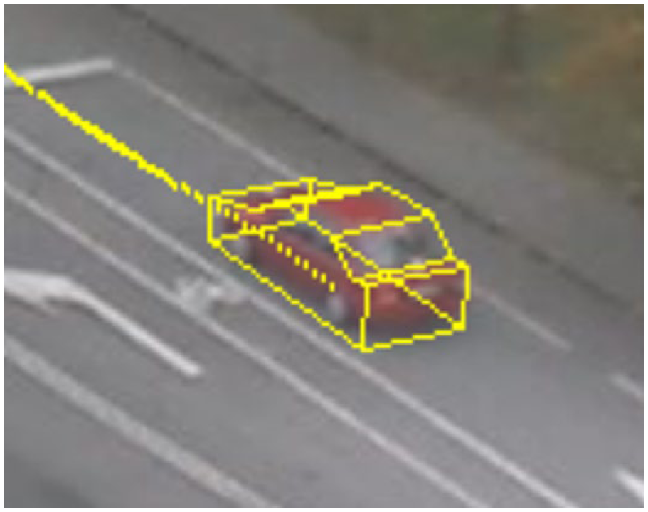
Wire-frame model.

The following calibration scenarios were tested.

All available calibration points with measured world coordinates used (Figure 11);

Few poorly located points with world coordinates taken from a Google Maps satellite image (Figure 12);

Multi-camera set-up calibration according to the algorithm described in Experiment 3. The initial calibration of both cameras was undertaken with few and unfavorably located points and the world coordinates taken from a satellite image (Figure 13).

Figure 11.

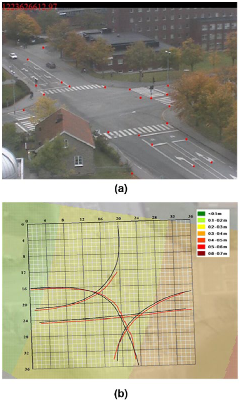
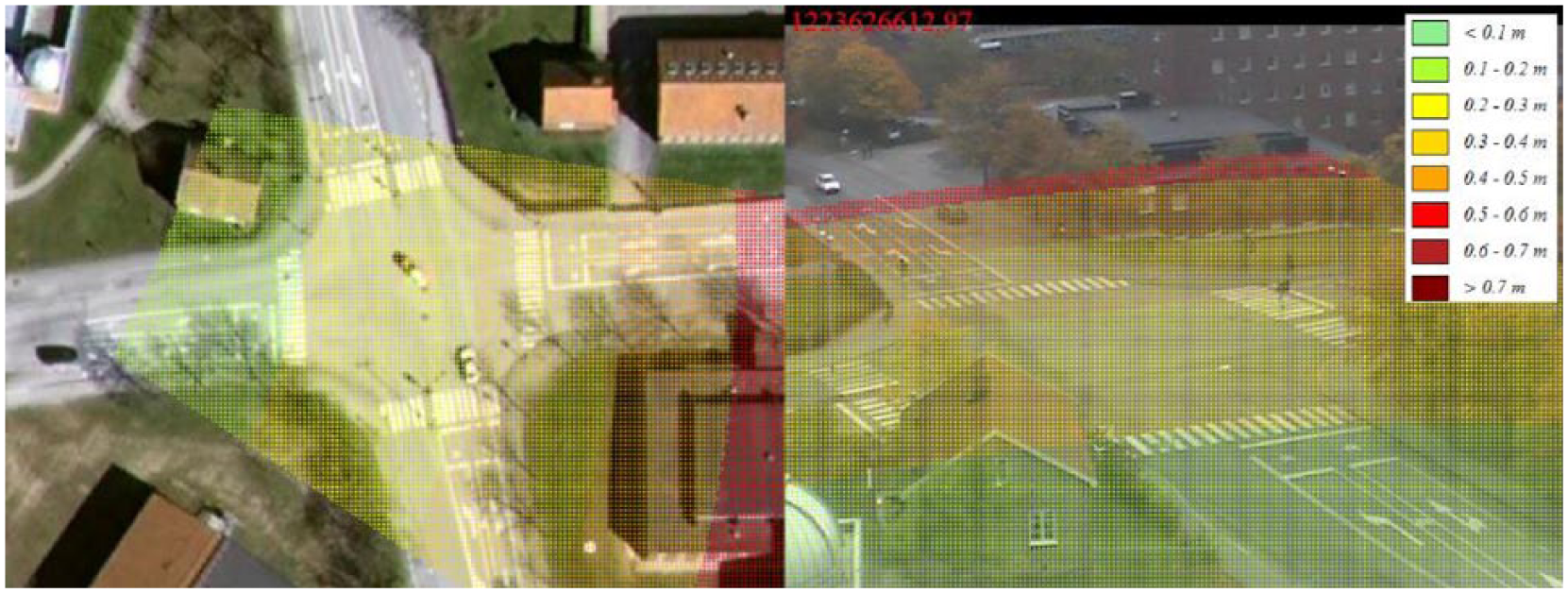
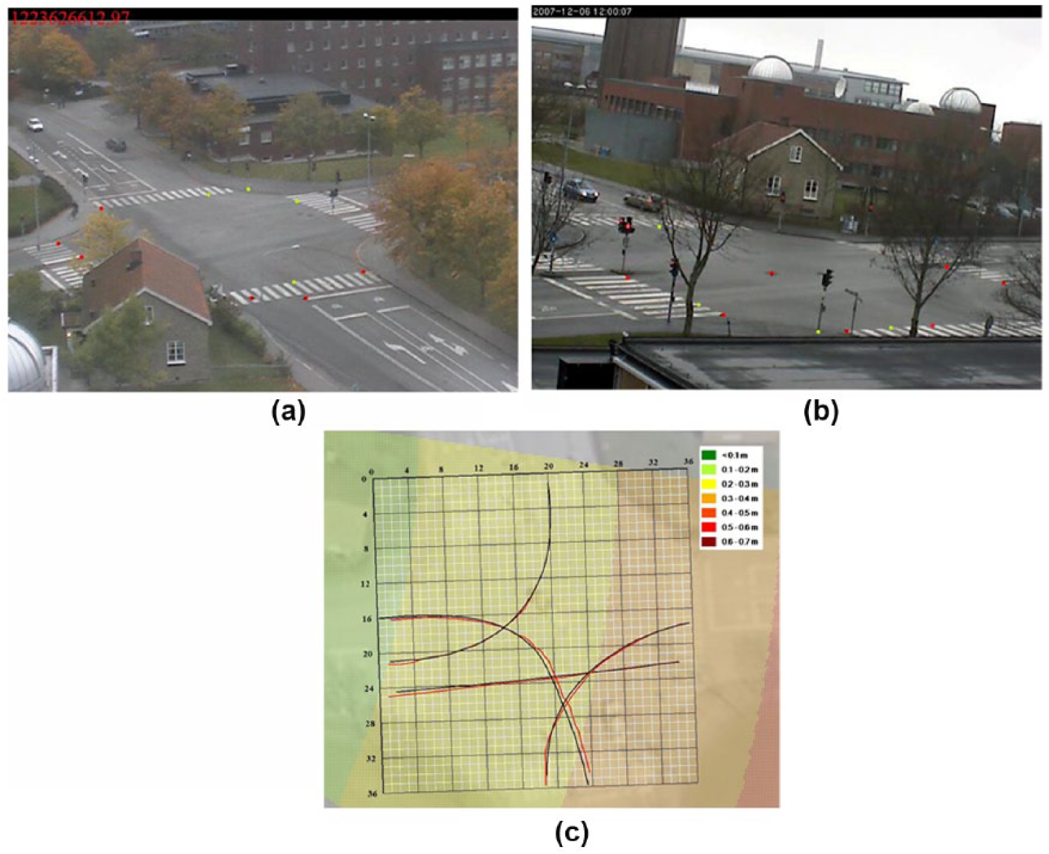
Calibration based on measured 3D points: (a) calibration points and (b) trajectories obtained from GNSS (black) and video (red). The colors in the background show the “price” of an image pixel error in world distance units; it should be considered that as the price increases, a lower accuracy of the video-based trajectory points should be expected.

Figure 12.

Calibration based on few points and world coordinates obtained from a satellite image: (a) calibration points and (b) trajectories from GNSS (black) and video (red).

Figure 13.

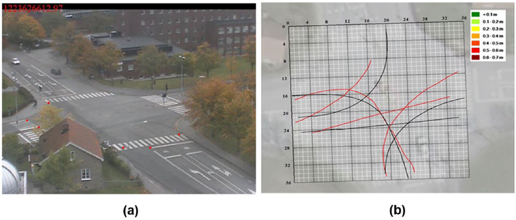
Multi-camera calibration: (a) and (b) points used for initial calibration (red) and “common points” without known world coordinates (green); (c) trajectories obtained from GNSS (black) and video (red).

Not surprisingly, calibration based on few points (second scenario) failed completely. However, when the same set of points was used together with another camera view in a multi-camera calibration, highly satisfactory results were obtained. In fact, it appears that the multi-camera calibration provides a better fit with the GNSS-obtained trajectories compared with the calibration based on accurately measured points in the first scenario. An explanation might be that the availability of the height data for points in the first scenario allows for an estimation of the correct horizontal plane on which road users can move, even though the actual road surface was not horizontal. The point coordinates obtained from the satellite image lack height data; thus, the estimated zero-plane is not horizontal, and it is more closely adjusted to the actual road surface.

Generally, the assumption that road users are moving on the zero-plane might result in inaccuracies if the studied area is not flat (for example, if one of the intersection legs had a more acute incline compared with the rest of the intersection). This becomes even more probable if a larger area is studied (e.g., covered with several cameras). To compensate, it might be necessary to create a model of the road surface (for example, by interpolating the heights of the measured points); instead of always assuming that road users travel on the zero-plane, the actual height calculated by the surface model could be used.

Conclusions

Carefully choosing calibration points appears highly crucial to the quality of the final calibration model. Ideally, these points should cover evenly the entire camera image, but their locations around the studied area (e.g., zebra markings around an intersection) might still be a reasonable compromise.

Camera height affects the accuracy of the measurements, but to a lesser extent than calibration point selection.

Inaccurate world coordinates of the calibration points (e.g., taken from a blurry satellite image) result easily in an inadequate calibration model. Additional visual control of the obtained calibration (e.g., by drawing a grid on the zero-plane) is highly recommended.

The use of several camera views with common points may greatly improve the calibration of each single camera. The additional camera views do not necessarily require another video camera installation, they can simply be taken with a mobile phone or camera, thus minimizing the additional work required.

The introduction of a road surface height model might be an additional step toward improving the accuracy of measurements from videos. This might be particularly important in the case of a large study area in which significant height variations are possible; thus, the assumption that road users move on the zero-plane might be insufficient.

In this study, we have not investigated the temporal aspect of the measurements from videos (for example, the accuracy of speed and acceleration calculated based on the positions measured from a video). This aspect should be addressed in future research.

Footnotes

Acknowledgements

This work has received funding from the European Union’s Horizon 2020 research and innovation program under grant agreement No. 635895. Some data were collected in a project financed by Vinnova, Sweden’s innovation agency.

Author Contributions

The authors confirm contribution to the paper as follows: study conception and design: A.L., M.N.; data collection: A.L.; analysis and interpretation of results: A.L.; draft manuscript preparation: A.L., M.N. All authors reviewed the results and approved the final version of the manuscript.

The Standing Committee on Highway Traffic Monitoring (ABJ35) peer-reviewed this paper (18-01963).

This publication reflects only the authors’ views. The European Commission and Vinnova are not responsible for any use of the information it contains.

References

Laureshyn

de Goede

Saunier

Fyhri

Cross-comparison of Three Surrogate Safety Methods to Diagnose Cyclist Safety Problems at Intersections in Norway. Accident Analysis & Prevention, Vol. 105, 2017, pp. 11–20. http://dx.doi.org/10.1016/j.aap.2016.04.035.

Saunier

Sayed

Ismail

Large Scale Automated Analysis of Vehicle Interactions and Collisions. Transportation Research Record: Journal of the Transportation Research Board, 2010. 2147: 42–50.

Madsen

Lahrmann

Comparison of five bicycle facility designs in signalized intersections using traffic conflict studies. Transportation Research Part F: Traffic Psychology and Behaviour, No. 46 (Part B), 2017, pp. 438-450. https://doi.org/10.1016/j.trf.2016.05.008.

van der Horst

A. R. A.

Thierry

M. C.

Vet

J. M.

Rahman

A. F.

An Evaluation of Speed Management Measures in Bangladesh Based upon Alternative Accident Recording, Speed Measurements, and DOCTOR Traffic Conflict Observations. Transportation Research Part F: Traffic Psychology and Behaviour, Vol. 46, 2017, pp. 390–403. http://dx.doi.org/10.1016/j.trf.2016.05.006.

St-Aubin

Miranda-Moreno

Saunier

A Surrogate Safety Analysis at Protected Freeway Ramps Using Cross-Sectional and Before-After Video Data. Presented at 91st Annual Meeting of the Transportation Research Board, Washington, D.C., 2012.

Polders

Cornu

De Ceunynck

Daniels

Brijs

Hermans

Wets

Drivers’ Behavioral Responses to Combined Speed and Red Light Cameras. Accident Analysis & Prevention, Vol. 81, 2015, pp. 153–166. http://dx.doi.org/10.1016/j.aap.2015.05.006.

De Ceunynck

Dorleman

Daniels

Laureshyn

Brijs

Hermans

Wets

Sharing is (s)caring? Interactions between Buses and Bicyclists on Bus Lanes Shared with Bicyclists. Transportation Research Part F: Traffic Psychology and Behaviour, Vol. 47, 2017, pp. 301–315. http://dx.doi.org/10.1016/j.trf.2016.09.028.

Archer

Indicators for Traffic Safety Assessment and Prediction and Their Application in Micro-Simulation Modelling: A Study of Urban and Suburban Intersections. Doctoral thesis. Department of Infrastructure, Royal Institute of Technology, Stockholm, 2005.

Huang

Liu

Wang

Identifying if VISSIM Simulation Model and SSAM Provide Reasonable Estimates for Field Measured Traffic Conflicts at Signalized Intersections. Accident Analysis & Prevention, Vol. 50, 2013, pp. 1014–1024. http://dx.doi.org/10.1016/j.aap.2012.08.018.

10.

Radwan

Abou-Senna

Determine if VISSIM and SSAM could Estimate Pedestrian-Vehicle Conflicts at Signalized Intersections. Journal of Transportation Safety & Security, 2017 (online). https://doi.org/10.1080/19439962.2017.1333181.

11.

Heikkilä

Silven

A Four-Step Camera Calibration Procedure with Implicit Image Correction. Proc., IEEE Conference on Computer Vision and Pattern Recognition, IEEE, New York, 1997, pp. 1106–1112.

12.

Tsai

R. Y.

A Versatile Camera Calibration Technique for High-Accuracy 3D Machine Vision Metrology Using Off-the-Shelf TV Cameras and Lenses. IEEE Journal of Robotics and Automation, Vol. RA-3, No. 4, 1987, pp. 323–344. https://doi.org/10.1109/JRA.1987.1087109.

13.

Zhang

A Flexible New Technique for Camera Calibration. IEEE Transactions on Pattern Analysis and Machine Intelligence, Vol. 22, No. 11, 2000, pp. 1330–1334.

14.

Klein

L. A.

ITS Sensors and Architectures for Traffic Management and Connected Vehicles. CRC Press, Taylor & Francis Group, Boca Raton, FL, 2018. https://doi.org/10.1201/9781315206905.

15.

T-Analyst. Software for Semi-Automated Video Processing. www.tft.lth.se/software. Accessed April 4, 2017.

16.

Willson

. Tsai Code Implementation. http://www-2.cs.cmu.edu/afs/cs.cmu.edu/user/rgw/www/TsaiCode.html. Accessed January 15, 2014.