
Abstract
High-resolution vehicle data including location, speed, and direction is significant for new transportation systems, such as connected-vehicle applications, micro-level traffic performance evaluation, and adaptive traffic control. This research developed a data processing procedure for detection and tracking of multi-lane multi-vehicle trajectories with a roadside light detection and ranging (LiDAR) sensor. Different from existing methods for vehicle onboard sensing systems, this procedure was developed specifically to extract high-resolution vehicle trajectories from roadside LiDAR sensors. This procedure includes preprocessing of the raw data, statistical outlier removal, a Least Median of Squares based ground estimation method to accurately remove the ground points, vehicle data clouds clustering, a principle component-based oriented bounding box method to estimate the location of the vehicle, and a geometrically-based tracking algorithm. The developed procedure has been applied to a two-way-stop-sign intersection and an arterial road in Reno, Nevada. The data extraction procedure has been validated by comparing tracking results and speeds logged from a testing vehicle through the on-board diagnostics interface. This data processing procedure could be applied to extract high-resolution trajectories of connected and unconnected vehicles for connected-vehicle applications, and the data will be valuable to practices in traffic safety, traffic mobility, and fuel efficiency estimation.
High-resolution vehicle data including continuous location, speed, and direction are important to connected-vehicle applications, micro-level traffic performance evaluation, and adaptive traffic control. Connected-vehicle technologies, applications and potential benefits have been studied since 2003 when the U.S. Department of Transportation (U.S. DOT) initiated the Vehicle Infrastructure Integration (VII) program ( 1 ). The connected-vehicle system provides longer detection distance for drivers (or autonomous vehicles) and pedestrians to “see” around corners or “through” other vehicles so that threats can be perceived earlier. A long list of connected-vehicle applications ( 2 – 4 ) was intended to be developed to test technical functionality of the connected-vehicle system, but the testing has not well demonstrated the effectiveness or end-user benefits of the identified applications in the real world. This problem was caused by the scope of proof-of-concept, and the current connected-vehicle system is highly reliant on information broadcast by each vehicle. The maximum safety benefits of current connected-vehicle deployment would need all vehicles to have connected-vehicle devices and broadcast their information in real time. However, mixed traffic with connected-vehicles and unconnected-vehicles will exist in the next decades or even longer. Therefore, supplemental data to help the connected-vehicle deployment needs to be considered.
High-resolution micro traffic data can be collected by conventional probe vehicles with the GPS logging function. However, probe vehicles provide only sample data of the traffic fleet on roads, while the connected-vehicle system needs the data of all road users. The traditional traffic sensors such as loop detectors, video detectors, Bluetooth sensors and radar sensors mainly provide macro traffic data such as traffic flow rates, average speeds and occupancy ( 5 ) or spot vehicle speed, so the existing sensors cannot provide the continuous micro traffic data needed by connected vehicles. Even the popular crowd-sourced data, such as real time travel time data from Wave, is still macro-level traffic information. A new method to collect high-resolution micro traffic data for the connected-vehicle system is needed to help the current connected-vehicle deployment and future connected-vehicle applications. The high-resolution micro traffic data will also change existing traffic safety engineering and traffic operation. For example, the micro-level trajectories of vehicles and pedestrians at intersections can be used to analyze intersection traffic safety and signal performance with much more detail than the traditional safety and performance analysis.
A light detection and ranging (LiDAR) sensor transmits and receives laser signals at a high frequency to obtain the point clouds of surrounding objects ( 6 ). The LiDAR sensor is better than video image processing for its insensitiveness for light variation. The LiDAR sensor usually has a finer resolution compared with Radar. Moreover, the existing Radar sensors deployed in the U.S. only report the spot speed and spot traffic volumes, which cannot support applications of connected vehicles. LiDAR can scan a 360º horizontal range and is able to detect the direction of arrival as well as the number of vehicles accurately. However, it has a relatively high cost compared with other sensors, so its usage was limited. The popularity of autonomous vehicles brought opportunities to the LiDAR sensor. The LiDAR sensor is widely adopted for object perception and recognition in the autonomous vehicle field. As an indispensable component for autonomous vehicles, the price of LiDAR sensors has decreased significantly in recent years. For example, the 2017 LeddarTech Vu-8, which has 215 m of detection range, 100º of horizontal sensing range, and weighs 107 g is now priced at $750. The LiDAR sensor used in this research paper was Velodyne’s VLP-16; it was $7,999, with 100 m of detection range, 360º of horizontal sensing range, and weighed 830 g. This trend enables traffic engineers to utilize cheaper LiDARs to obtain high-resolution datasets.
Extensive research has been conducted to apply LiDAR and optical sensors for detecting and tracking vehicles in autonomous sensing systems. The most widely adopted approach to pedestrian and vehicle detection is to combine LiDAR features and vision-based features ( 7 ). The advantage of using a LiDAR associated with a vision system is that the laser sensor is not very sensitive under extreme weather changes, and the distance or depth measurement is accurate, while at the same time the vision system includes rich information. In Cristiano’s research ( 8 ) for LiDAR data processing, a 15-dimensional LiDAR-based feature vector, Histogram of Oriented Gradients and Covariance image descriptors are extracted. Himmelsbach ( 9 ) proposed a fast response 3D object perception procedure which could be applied to autonomous vehicles. The uniqueness of his method is that the segmentation was done in a 2.5 D occupancy grid, and classification was done in 3D point clouds. These literature reviews suggest that the LiDAR data processing procedures for autonomous vehicles provide good references for processing the roadside LiDAR sensor data. However, the LiDAR application for roadside traffic surveillance is different from LiDAR application on autonomous vehicles. First, the LiDAR sensors are installed at a fixed place instead of a moving vehicle. Secondly, the system should be able to constantly detect and track vehicles even without a good shape of a vehicle (shaped by 3D LiDAR points). This requires the data processing algorithm to be scalable and robust to track the vehicle with fewer LiDAR points. Thirdly, the LiDAR sensor should be able to track the speed without help of other types of sensors. More sensors, especially different types of sensors, mean more maintenance labor and higher budgets, which may cause unacceptable cost for cities or states. Therefore, a data processing procedure was developed specifically for roadside LiDAR sensor data, which could track vehicles with low LiDAR point density and without the support of other optical sensors. These trajectories could be applied to traffic performance evaluation, safety countermeasures, and traffic operation. The developed procedure is especially important for filling the data gap of existing connected-vehicle deployment.
This paper is organized as follows. The major data processing procedure is presented first. Next, is demonstrated the testing results with LiDAR data collected at different intersections and roads. Finally, all the findings are summarized, and future research is introduced. The data processing procedure proposed in this paper could automatically extract high-resolution vehicle trajectories from LiDAR data.
Procedure of Extracting High-Resolution Trajectories
The LiDAR sensor used in this research has the following specifications: 16 channels, 300,000 points per second, 360º horizontal field of view (FOV) as well as a 15º vertical FOV. The data processing procedure proposed in this paper includes preprocessing of the raw data, statistical outlier removal, a Least Median of Squares (LMedS) based ground estimation method to remove the ground points accurately, vehicle data clouds clustering, a principle component-based oriented bounding box method to estimate the location of vehicle, and a geometrically-based tracking algorithm.
Raw Data Processing
The sensor manual suggested not using the points within a 2-m radius. Hence the points in the 2-m-radius range to the sensor were excluded first. The region of interest (ROI) was then determined based on the road locations and geometry. Four reference points have been selected. Linking these four points would yield a cuboid area. The space outside of this cuboid area was considered a region of no interest. By trimming out the region of no interest, the buildings, trees, traffic signs and other irrelevant objects would be filtered out from the dataset. Filtering of irrelevant objects decreases the data size for processing, so it increases the efficiency of the follow-up steps. This step also reduces the influence of uninteresting objects. Figure 1 compares a raw data frame and a preprocessed data frame.
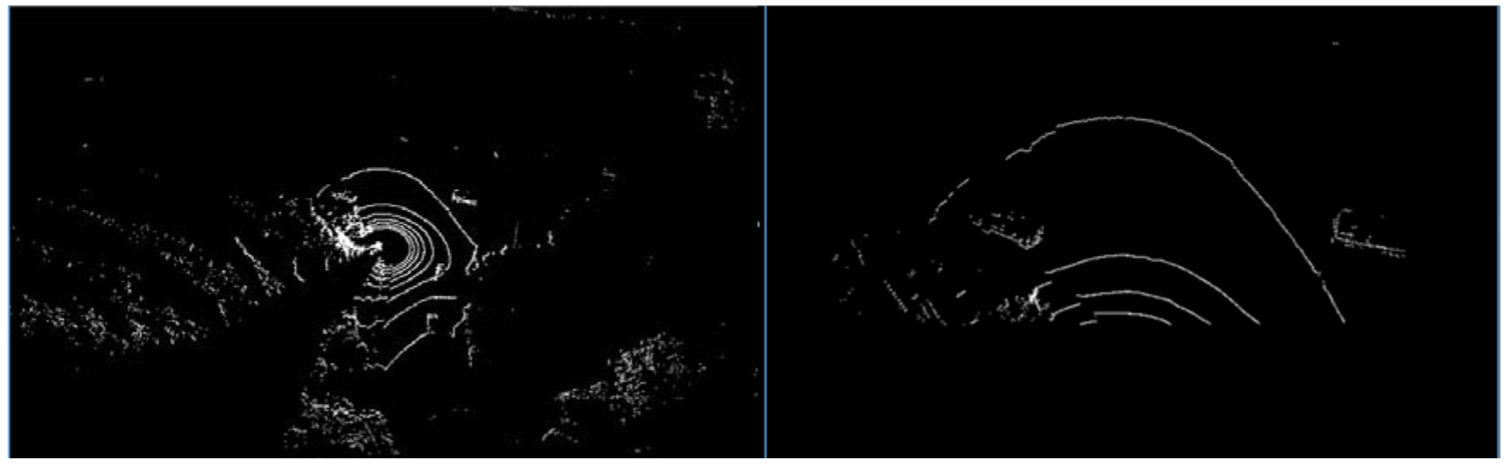
A raw data frame (left) and the same data frame after preprocessing (right).
Statistical Outlier Removal
This step removes the noise data points near the objects. These noises in each data frame complicate the vehicle identification and tracking and introduce errors of vehicle locations and speeds. A statistical outlier remover algorithm ( 10 ) was applied at this step. This sparse outlier removal algorithm is based on the computation of the distribution of point to its K neighbor’s distances in the input data frame. For each point, the algorithm will compute the mean distance from it to all its neighbors. By assuming that the resulted distribution is Gaussian, all points whose mean distances are outside an interval defined by the global distances mean and standard deviation can be considered as outliers and trimmed from the data frame. Figure 2 presents the comparison of before and after the outlier removal step.
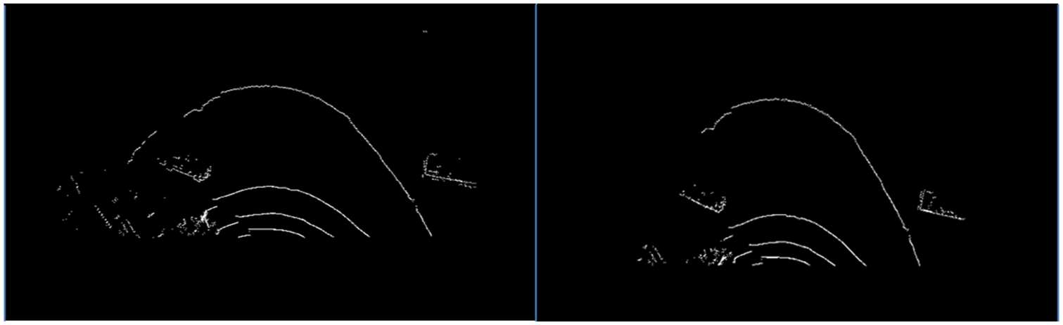
Data frame before outlier remover (left) and after outlier remover (right).
Ground Plane Identification and Segmentation
Correctly and accurately identifying and segmenting the ground plane is an essential step for the proposed data processing procedure. The ground plane here is defined as a group of concentric circle points when LiDAR scanning the ground. Therefore, these sparse noises are subject to being identified and removed. The ground plane is recognized as the noise of the data frame, thus random sample consensus (RANSAC) ( 11 ), an iterative method to estimate the parameters of mathematical models, was adopted. The input of RANSAC method contains three parts: the data to be processed, a candidate mathematical model fit into the data frame outliers, and parameters related to the estimation of the model. Here a mathematical model was considered as a surface function which could represent the ground plane. There are two key parameters. The first parameter is the number of iterations. The iteration limit was set to 200 by experiments regarding efficiency and successful rate ( 12 ). The second allowed error parameter is the allowed deviate angle. This deviate angle was set to 15º, which means the direction of the estimated surface could not deviate 15º away from the vertical vector (0, 0, 1). If the estimated surface has a degree larger than this, it will automatically trigger failure segmentation.
The RANSAC iteration method contains four steps. A random subset of the original data was selected first. This subset of data was called hypothetical inliers. Then, the predefined model was fitted to the set of hypothetical inliers. Next, all other data are tested against the fitted model. Those points that fitted this model well would be incorporated into this model. This larger estimation model is considered as a good model if there are enough points in the model. Finally, if the model is not good, another subset of data frame was randomly selected and estimated. RANSAC can estimate the surface function parameters even with significant noises presented in the data frame, but it has no guarantee of delivering optimal solutions within limited iterations. This suggests that by computing a greater number of iterations the optimized solution was approximated. Other variants of RANSAC ( 13 ) were also tested. RANSAC solves the selection problem as an optimization problem with a bounded loss function. The loss function is defined as a summation of geometric distance for all the points to the estimated plane. When a point is within allowed distance, this point is considered to belong to the estimated plane hence the loss value for this point is set to zero.
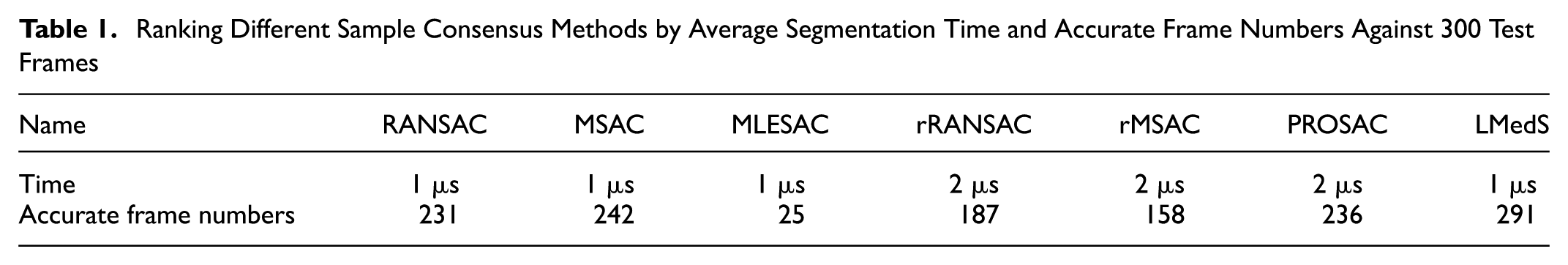
LMedS is a modified RANSAC method. LMedS method does not need any tuning variable because it tries to minimize median squared error ( 14 ). Hence it is considered as a robust estimation. Robust here means fast and insensitive to noises of a data frame. Different modified RANSAC methods were tested against the same data frames; the LMedS model was found to achieve a high accuracy while only consuming a limited computation time, as presented in Table 1. Therefore, it was adopted for ground plane segmentation method in this research. The accurate frame in the table was defined as a frame whose ground plane was perfectly removed and there is no scanning line on the ground left for this frame after ground plane segmentation.
Ranking Different Sample Consensus Methods by Average Segmentation Time and Accurate Frame Numbers Against 300 Test Frames
It should be noted that none of the mentioned methods could guarantee a perfect segmentation for all tested data frames. In this research, a follow-up cleaning algorithm was designed. This algorithm removes a 0.2 m thick cuboid by utilizing the plane model parameters, instead of just removing points in a plane. This follow-up algorithm deletes residual ground points around the plane while keeping the vehicle clouds points integrated and completed. Figure 3 indicates the effect of the ground removal step.
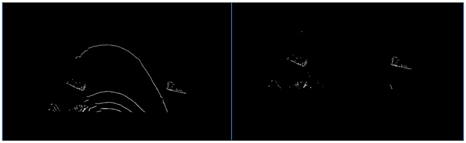
Data frame before ground plane remover (left) and after ground plane remover (right).
Vehicle Clustering
A clustering method is needed to cluster points of different vehicles. The algorithm applied in this research was developed by Rusu ( 15 ). This clustering algorithm was named Basic Clustering Techniques. The key part is letting the system understand what an object point cluster is, and what makes it different from another. A threshold is required as the input to this algorithm, which is the minimal distance between two cloud sets. Rusu proposed to approximate nearest neighbors via the kd-tree structure ( 16 ). First, an empty list of clusters was set up, and an empty queue was set up. Then for a random point P in a LiDAR data frame, P is added to the current queue. The algorithm then searches points within a user-defined radius from point P. These neighbor points are marked as processed points and will not be added to another queue. After the search for point P and adding all its neighbor points into the current queue, the corresponding queue will be saved, then a new one is created. The next candidate point is randomly selected, and its neighbor points are searched in the same method. The algorithm terminates when all points have been stored in queues. After clustering, the points are grouped into individual objects and subject to extraction of the useful information. Figure 4 demonstrates clustered result.
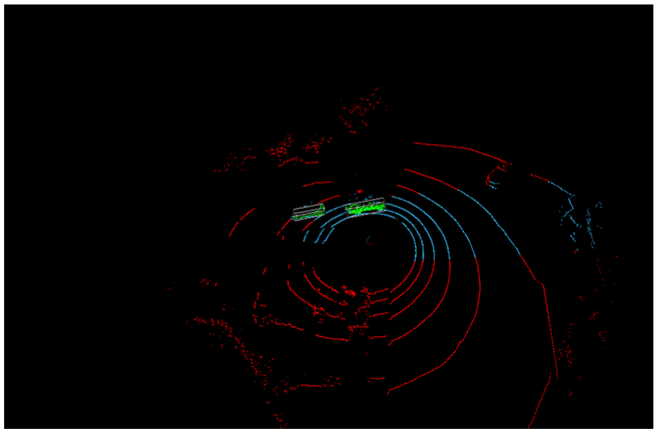
Results of LiDAR points clustering: red points indicate raw data; blue points indicate data after preprocessing; green points indicate clustered vehicles.
Vehicle Identification
Because the LiDAR sensor would penetrate the window of vehicles, or simply the scanning could not cover every corner of the vehicle, the vehicle identification step is to identify the location and shape of vehicles accurately. The space center of a cluster is first identified to represent the location of a vehicle. However, the center of a vehicle shifts frame by frame due to the incomplete structure of objects. The LiDAR sensor can only detect a part of a vehicle body in a frame, so the detected part changes when the vehicle moves. Thus, a reconstruction method is used to restore the shape of vehicles before identification of the actual location of vehicles. It is to find the minimum-volume oriented bounding box (OBB) of a given finite set of N points. There are several methods to identify the OBB for a given finite set of points: O’Rourke’s Algorithm, brute-force methods, principal components analysis (PCA) based methods and some other method like (1+ε)-Approximation ( 17 ). In this research, a min-max PCA-based OBB method was used to identify vehicle boundaries. This method first calculates the principles (eigenvectors), and then a reference coordinate system is constructed based on these eigenvectors. The original vehicle cluster is translated into this new reference coordinate system, and a bounding box is constructed for the vehicle. This bounding box is then translated back to the original coordinate system and used as the optimum bounding box for this vehicle. The front corner point and back corner point, which are closest to the sensor, are identified as a key data pair to represent the location of this vehicle. Figure 5 indicates the identified vehicle boundary and the points used to track a vehicle.
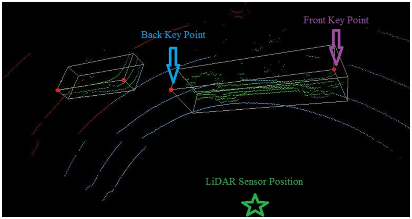
Identified vehicle boundary and key data pair.
Vehicle Tracking
Finally, an object tracking algorithm was applied to track vehicle trajectories. This tracking algorithm utilizes the geometric location information of vehicle key data pair to identify key points in different frames belonging to same vehicles. The algorithm tracks the front key point when the vehicle is approaching the sensor and tracks the back corner key point when the vehicle is leaving the sensor.
Figure 6 describes the whole data processing procedure.
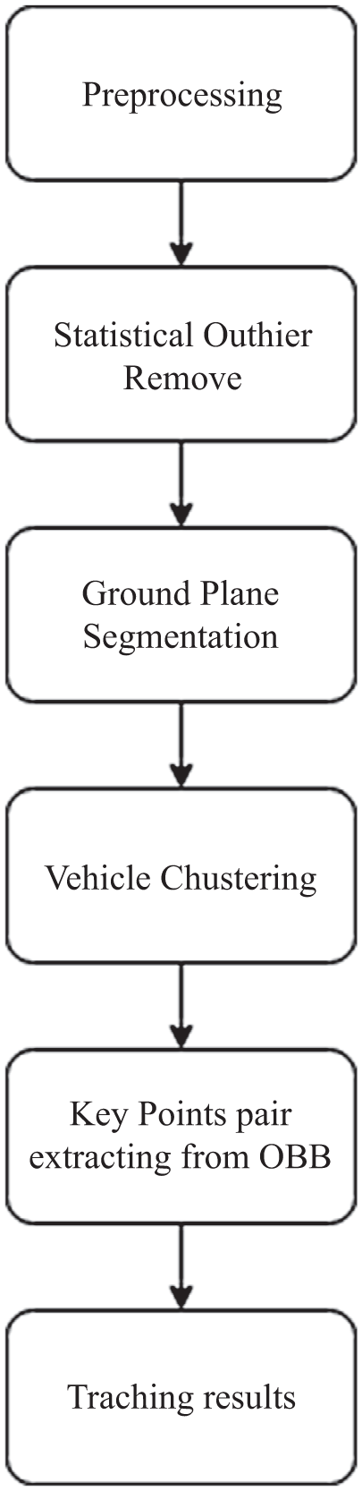
Flow chart of vehicle speed tracking with roadside LiDAR.
Testing Data Sets and Results
The data processing procedure has been tested with data collected at three sites for different traffic scenarios. To compare the tracking results and actual vehicle speeds, the authors installed a logging system at a testing vehicle. The logging system read and stored vehicle speeds from the on-board diagnostics (OBD) interface of the vehicle. This dataset was collected at the University of Nevada, Reno’s northern parking lot. Figure 7 presents the comparison of the extracted speeds from LiDAR data and the logged speeds of the testing vehicle. The tracking results of both directions match to the OBD speed very well. This indicates that this data processing procedure is precise and able to track vehicles in both directions.
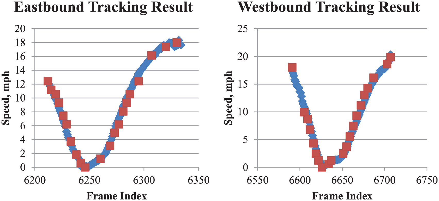
Parking lot tracking results: blue dots indicate tracking result; red dots indicate OBD speed.
Another dataset was collected at the intersection of Evans Street and Enterprise Road in Reno, Nevada, which is a two-way-stop-sign intersection with four legs. Trajectories of two vehicles are shown in Figure 8. The leading vehicle stopped at the eastbound Enterprise Road, waited for a gap, and then crossed the intersection. The follow-up vehicle decreased speed and waited for the leading vehicle to pass the street, as the frame index 4000–4500 indicates. The follow-up vehicle then accelerated and approached to stop bar. When there was a gap, it accelerated sharply and crossed the intersection. This experiment demonstrates the effectiveness of data processing framework in a multiple-vehicles passing environment.
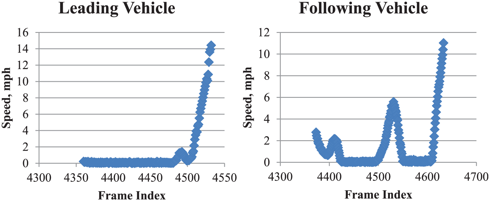
Two vehicle tracking results at the intersection of Evans street and Enterprise road (two-way-stop-sign scenario).
The data processing procedure was then applied to the data collected on Kietzke Lane. Kietzke Lane is an arterial road with a speed limit of 40 mph in Reno, Nevada. Figure 9 shows the tracking results. It should be noted that some vehicles slowed down when approaching the sensor. It is possibly the data collection that attracted drivers’ attention and caused the speed reduction. The flat speed profile suggests higher speed tracking is also effective and stable.
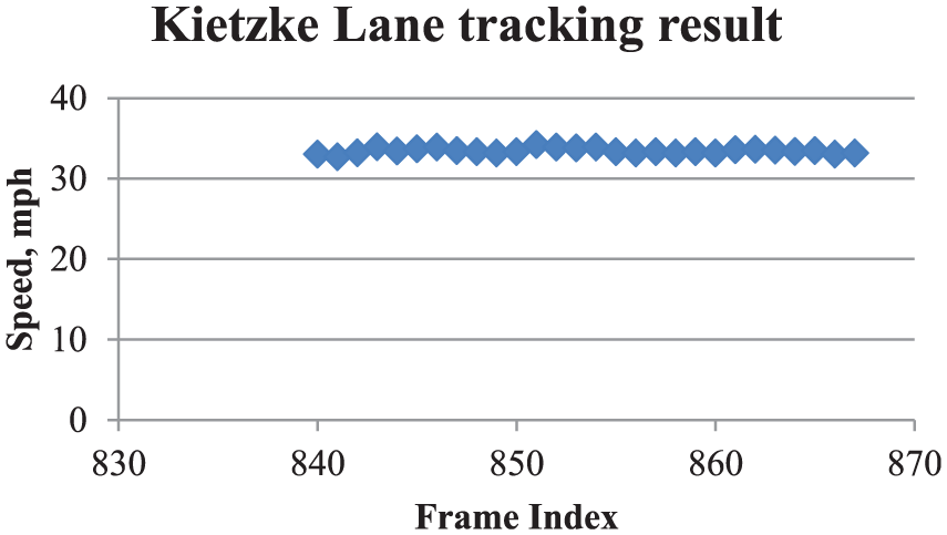
One vehicle tracking result on Kietzke lane (free-flow scenario).
To test whether this data processing procedure obtains accurate traffic volumes, the research group tested this procedure against another additional dataset collected at the intersection of 15th Street and Virginia Street, Reno Nevada. Vehicle information from 1000 frames of data was extracted by hand and was considered as valid references for comparison. Out of 36 passing vehicles, 35 vehicles were accurately tracked. One vehicle was missing because a near-sensor vehicle proceeded at the same speed with the missing vehicle, and this near-sensor vehicle blocks the missing vehicle’s whole body all the way.
Another finding from this research is that the tracking speed of vehicles passing the sensor using this data processing procedure might suddenly drop or increase. The scanning shape of a vehicle may not be complete when this vehicle is close to the sensor, so when tracking the vehicles, the front key point would be cut short. This would cause the drop of the tracking speed. A sudden increase of speed is also possible because the sensor saves the next frame’s vehicle data into the current frame, which would cause a sudden extension of the front tracking point. The first situation is not likely to happen when there is a distance, preferably 3 m, between the sensor and vehicles. These 3-m distances create space for LiDAR to obtain the complete shape of the vehicles. The second situation is caused by VLP-16 LiDAR itself therefore could not be avoided. Although these scenarios are not common, they can be identified, smoothed, and reported before generating the actual tracking speed profiles in the developed method.
Conclusions and Future Research
This paper presented a data processing procedure to extract vehicle trajectories from roadside LiDAR data. The procedure includes preprocessing of the raw data, statistical outlier removal, an LMedS based ground estimation method to accurately remove the ground, vehicle data clouds clustering, a PCA-based OBB method to estimate the location of a vehicle, and a geometrically-based tracking algorithm. The documented data processing procedure has been applied to a two-way-stop-sign intersection and free-flow traffic in the Reno area. The results have been compared and verified with speed data from a logger-equipped testing vehicle. A total of 18,000 frames data were collected and tested. The result suggests that the proposed data processing procedure could be used to track vehicle speed at stop-sign intersections and arterial roads, as well as parking lots. This research could be applied to other roads and intersections, and be extended to tracking vehicles in other types of traffic segments, such as four-way-stop-sign intersections or freeways.
This data processing procedure can be applied to extract high-resolution trajectories for various traffic applications. First, by utilizing the roadside LiDAR data processing procedure, connected vehicles could perceive unconnected vehicles. Secondly, traffic safety analysis could be conducted because high-resolution LiDAR data would reveal more details on the roads. Thirdly, traffic counts could be directly extracted from the data processing procedure regardless of daytime or nighttime. This would save time and effort for traffic engineers. Fourthly, this research would benefit operation performance evaluation. Signal evaluation, delay time evaluation or stop time evaluation all will benefit from this research. Finally, the self-detected device could be designed. The ordinary Rectangular Rapid Flash Beacon (RRFB) could be upgraded to detect and predict pedestrian behavior automatically. In summary, the proposed data processing procedure would benefit connected-vehicle applications, traffic safety analysis, traffic mobility analysis, operation performance evaluation and self-detected traffic device design.
Future research will investigate how to integrate multiple LiDAR sensors to extend the detection range. The extension of detection range requires additional algorithms to fuse multiple datasets, while real-time tracking demands the procedure be fast enough to generate and display result within 0.1 seconds. In particular, this paper has not researched bad weather datasets, such as heavy rain and snow, which will introduce noises to the dataset. It is even possible for them to blind the sensor. How to filter snow or rain noise, and still achieve a satisfactory detection range, speed, and accuracy remains to be researched.
Footnotes
Acknowledgements
This research was funded by the SOLARIS Institute, a Tier 1 University Transportation Center (UTC) under Grant No. DTRT13-G-UTC55 and matching funds by the Nevada Department of Transportation (NDOT) under Grant No.P224-14-803/TO #13. The authors gratefully acknowledge this financial support. This research was also supported by engineers with the Nevada Department of Transportation, the Regional Transportation Commission of Washoe County, Nevada, and the City of Reno.
Author Contributions
The authors confirm contribution to the paper as follows: study conception and design: Yuan Sun, Hao Xu; data collection: Hao Xu, Jianqing Wu, Jianying Zheng, Kurt M. Dietrich; analysis and interpretation of results: Yuan Sun, Hao Xu; draft manuscript preparation: Yuan Sun, Hao Xu. All authors reviewed the results and approved the final version of the manuscript.
The Standing Committee on Information Systems and Technology (ABJ50) peer-reviewed this paper (18-00110).