Automated Validation and Interpolation of Long-Duration Bicycle Counting Data

Abstract

Bicycle flow data is crucial for transportation agencies to evaluate and improve cycling infrastructure. Average annual daily bicyclists (AADB) is commonly used in research and practice as a metric for cycling studies such as ridership analysis, infrastructure planning, and injury risk. AADB is estimated by averaging the daily cyclist totals measured throughout the year using a long-term automated bicycle counter, or by using long-term bicycle counting data to extrapolate data from a short-term counting site. Extrapolation of a short-term bicycle counting site requires an accurate and complete set of daily factors from a group of references: long-term bicycle counters. In practice, validation of reference data is done manually, an exercise that is time-consuming but crucial as significant error can be introduced into AADB extrapolation if reference data are not validated. This paper proposes an automated method to validate long-term bicycle count data and interpolate anomalous portions of data. As part of this work, the methods are validated using a relatively large dataset of automated bicycle counts. For validation of our approach, data anomalies are created artificially in a way that removes data (first trial), or reduces counts to 25% or 40% of the measured bicycle counts (second and third trials), for 6 hours, 12 hours, and full days. Of the more than 100 generated anomalies, the validation process flagged approximately 90% in the first and second trials and 80% in the third trial. The average absolute relative error of the interpolated daily values was approximately 10% for all three trials.

Bicycle flow data is crucial for transportation agencies to evaluate and improve cycling infrastructure. Transportation agencies can use bicycle flow data at locations across a network to help prioritize intersections awaiting road treatments, to determine which intersections require bike signal phasing, and to estimate exposure in traditional crash-based safety analysis for cyclists ( 1 ). Measuring flow and estimating daily averages is considerably simpler for motorized vehicles as compared to bicycles. Firstly, cyclists are harder to count than vehicles using traditional automated counting systems; vehicles are big and typically occupy a predictable space making them easy to count using automated counting technologies. Secondly, vehicle flows tend to be large and daily volume is stable over time, therefore short-duration counts can be used to predict daily averages with a relatively high-level of accuracy. Bicycle flows, on the other hand, tend to be smaller and vary significantly as a function of time and weather. Thus, the estimation of daily averages from short-duration counts is a laborious process and prone to error.

Average annual daily bicyclists (AADB) is the standard metric used by researchers and practitioners to quantify cycling flow, referred to as exposure, volume, ridership, or activity on bicycle facilities, at intersections or on road sections ( 2 , 3 ). Automated bicycle counting systems, used for measuring bicycle ridership, fall into two categories: long-term counters that run continuously at one location for multiple years, and mobile counters that capture a short duration of cycling demand (typically from 1 day to a month, and ideally for longer than a week) ( 3 ). The data from long-term counters can be used to calculate the AADB at a location when installed for more than 1 year, simply by averaging the daily bicycle demand throughout the year or bicycle season. Estimating the AADB with a short-term count is possible but requires extrapolation methods using knowledge of daily cycling demand patterns from appropriate references: long-term counting sites ( 3 , 4 ). Direct measurement of AADB using a long-term counter can be highly accurate but expensive. On the other hand, estimating AADB with a short-term count and extrapolation techniques, although relatively inexpensive, will produce results of varying accuracy. The accuracy of an AADB estimation is known to vary with several characteristics of the short-term count, including the time of year the data were collected, the count duration, and the level of cycling demand ( 3 , 5 ), as well as the goodness of match between the short-term count and the reference(s) used in extrapolation ( 6 ).

The accuracy of AADB estimation from short-term counts is also highly susceptible to error in the reference data, particularly in cases in which the reference experiences significant undercounting during the same period that the short-term count is taken. Undercounting of the reference count data can be difficult to identify if the counts are significantly reduced but non-zero. Undercounting can have many causes including automatic counter malfunction, temporary loss of power, and construction on or near cycling facilities. The most common source of undercounting may be the presence of utility, moving, or other vehicles diverting bicycles around the counting site.

At present, long-term bicycle count validation is done manually in practice, if at all, by researchers and practitioners. It is an arduous task involving many steps; however, it is crucial as long-term bicycle counting sites form the backbone of any city- or region-wide counting program. They provide rich data sets that can be used to evaluate bicycle ridership growth, in addition to being used as references to estimate AADB from short-term count data. However, when extrapolation is done, any errors in the long-term count data will be magnified as error in the AADB estimate of the short-term counting site. This is particularly true of zero- or highly suppressed counts in the long-term counts ( 6 ). An automated process that runs through all the steps of bicycle count data validation of long-term reference sites, by flagging and removing anomalous data and then replacing it through interpolation, would be useful in comprehensive bicycle counting programs and would make the AADB estimation from short-term counts more feasible in practice. This study builds on previous work related to semi-automated data validation of permanent bicycle counts ( 6 ). It has been demonstrated that nearby reference counting sites can be grouped together if their temporal cycling patterns are similar ( 4 , 6 , 7 ). Groups of similar counting sites can subsequently be used to identify periods of anomalous count data and to correct data during those periods.

The study objectives are to develop and fully automate a methodology for data validation and data interpolation to be used on reference counting data; and to test the methodology on long-term bicycle count data with simulated zero-count or suppressed-count anomalies. The simulated anomalies are limited to reduced or zero counts; however, this methodology also applies to anomalies that increase counts. The data used in this study come from 16 long-term bicycle counting sites in Arlington, VA. The proposed methodology is the result of collaboration with Eco-Counter, a manufacturer of automatic bicycle and pedestrian counting equipment. The methodology has been incorporated into software that will be accessible to jurisdictions with Eco-Counter equipment, but could be applied to continuous daily bicycle count data collected from any bicycle counting system.

Literature Review

A complete bicycle counting program, administered by a city, regional or state/provincial transportation agency, requires both long-term reference counting sites as well as short-term counting sites. A growing body of work has demonstrated several bicycle demand extrapolation techniques, with varying accuracy, for short-term counting sites ( 3 , 6 – 15 ). Nordback et al. demonstrated that average annual daily traffic extrapolation techniques for motor vehicle counting can be borrowed to estimate AADB ( 3 ). These techniques use day-of-week and month-of-year factors developed using continuous count data, taken over an entire year, from a group of counters located at similar cycling facilities. The authors explored how the error in AADB estimation is related to the duration of the short-term count, the month in which the short-term count was taken and the average bicycle demand. Nosal, Miranda-Moreno, and Krstulic examined four methods for AADB extrapolation including the disaggregated factor method, also known as the day-of-year factor method, which produced the best results ( 8 ). In this method, an expansion factor is computed for each day of the year using the raw daily counts and the annual, or seasonal daily average of a long-term reference counting site. This set of factors would typically be produced using a long-term counting site near the short-term counting site that requires extrapolation. The idea behind this method is that the proximity of the two counting locations ensures that weather affects cycling demand at both locations to a similar extent. The average absolute relative error (AARE) was compared for different extrapolation methods for short-term counts ranging from 1 day to 1 month’s duration.

Esawey studied AADB estimation error from short-duration counts using automated bicycle counters ( 11 – 14 ). In one study, daily and monthly adjustment factors were used to estimate AADB; estimation errors were then compared across different days of the week and across different months of the year ( 12 ). In another study, Esawey compared the estimation accuracy of methods used to estimate AADB including both traditional factor methods and day-of-year factor methods ( 14 ). Fournier proposed a sinusoidal model with a calibration factor to adjust for impact of seasonal demand change ( 16 ). The model can estimate monthly average daily bicycle counts and AADB using as little as two short-term counts, at high- and low-points in the cycling season. Hankey, Lindsey, and Marshall compared the day-of-year factor method to the more traditional day-of-week and month-of-year factor methods using data from off-street trail locations and found a significant reduction in AADB extrapolation error using the day-of-year factor method ( 9 ). A couple of studies have explored how AADB extrapolation error could be further reduced by correcting for specific sources of error. Beitel and Miranda-Moreno explored two approaches for extrapolating AADB that improved on previously reported work on the day-of-year factor method, and achieved more consistently accurate estimates than previously reported methods ( 6 , 8 , 9 ). One method utilized a filtering technique to remove AADB estimate outliers (Beitel and Miranda-Moreno, 2016). Figliozzi et al. proposed a methodology to reduce AADB extrapolation error by applying a correction function that used a regression model to account for weather and non-school days ( 10 ).

Several studies have demonstrated extrapolation techniques to estimate AADB from short-term counts ( 3 , 6 , 9 , 11 – 16 ). Each study assessed the accuracy of the extrapolation method developed using AARE (referred to in other studies as mean average percent error or MAPE) and some have compared errors for different methods developed in the literature ( 6 , 8 , 9 , 12 , 14 ). Furthermore, several studies have explored the relationship between AADB estimation error and short-term count duration, bicycle demand, time-of-year of the short-term count, and other factors ( 3 , 5 , 9 , 14 ). Some recent contributions have addressed important research gaps related to site selection and implementation of bicycle counting programs ( 17 – 19 ) and methodologies to assist in quality assurance and quality control ( 19 – 21 ). The Traffic Monitoring Guide, produced by the U.S. Federal Highway Administration, provides guidance on non-motorized counting programs, describes challenges in collecting non-motorized data, and includes case studies that define manual quality-control techniques that can be applied to bicycle count data ( 19 ). The national bicycle and pedestrian count archive, called Bike-Ped Portal, completed on behalf of the National Institute for Transportation and Communities, allows for nationwide data sharing and offers some built-in features including data visualization and zero-data detection ( 22 ). These contributions have helped make AADB extrapolation from short-term counts more feasible. However, a significant research gap remains that limits the applicability of AADB estimation from short-term counts in practice. No studies have developed a robust, automated technique for the validation of long-term reference count data.

Validating and correcting reference bicycle count data is crucial in achieving a high accuracy in AADB extrapolation, regardless of the extrapolation method subsequently used. Undercounting of the reference data can have a large impact on the accuracy of the daily AADB extrapolation of a short-term counting location because the daily bicyclist factors of the reference data appear in the denominator of the estimate ( 6 ). Therefore, a partial restriction of a bicycle facility, at a reference counting location, that reduces the bicycle counts by 75% during the period of the short-term count would produce an AADB estimation error at the short-term count location of 300%. In estimating AADB, Nosal manually removed all zero and missing data, resulting in a loss of 4% of data ( 8 ). Currently, the only available method for identifying undercounting and other anomalies is to manually analyze continuous data by hourly intervals. This is typically done by viewing data graphically; all anomalies that cannot be explained by variation in local weather are then flagged or removed ( 4 , 6 ). This method, though highly valuable, is arduous and time-consuming. It can also be challenging to spot data that is highly reduced yet non-zero due to a partial blockage of the bike facility. An automated method would be significantly less time-intensive and more complete than the manual methods that are used in practice. The automated validation method proposed in this study is an extension of a semi-automated validation method proposed by Beitel ( 6 ). In the case that data from multiple reference counters are available for an entire year (or cycling season) in a single city or region, then data validation and anomaly identification can be achieved by validating the daily factors of each counting site against the daily factors of other similar counting sites. An automated process that validates reference bicycle count data would provide practitioners with a tool that can help in the estimation of bicycle flows at many locations across city- or region-wide bicycle networks.

Methodology

Anomalous data are easily identified as periods when a counting location has a variation about its daily factor that is not mirrored at other, similar counting locations. The proposed process identifies similar counting sites for each reference site, detects days of the cycling season when similar sites have differing daily factors, and, if necessary, removes and interpolates the anomalous daily factor. The process consists of the following six steps:

(1) Calculate the daily factors for each long-term counting location. Each daily factor is calculated by taking the quotient of the bicycle count on that day and the annual, or seasonal, daily average. Note that the method for determining the daily factors was proposed by Nosal as part of the day-of-year factor method for estimating AADB and is used in this study in a different context, for validating reference data ( 8 ).

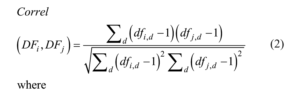
(2) Calculate the correlation between all possible pairs of reference sites. For each site i, calculate the correlation between the vector of daily factors and the vector of daily factors for each other site j, according to Equation 1 and simplified to Equation 2.

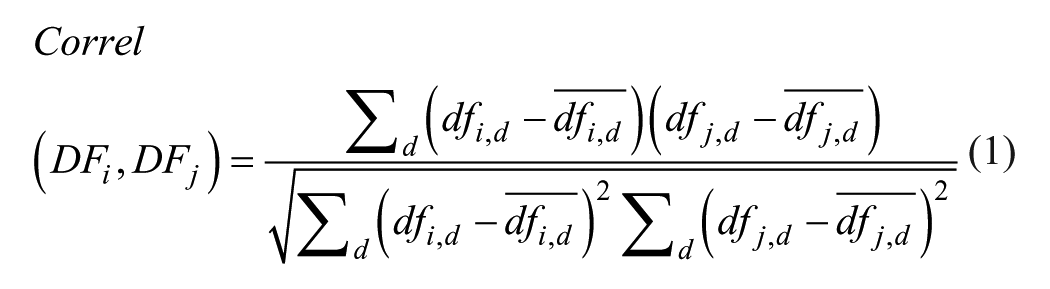
\begin{array}{l} C o r r e l \\ (D F_{i}, D F_{j}) = \frac{\sum_{d} (d f_{i, d} - \bar{d f_{i, d}}) (d f_{j, d} - \bar{d f_{j, d}})}{\sqrt{\sum_{d} {(d f_{i, d} - \bar{d f_{i, d}})}^{2} \sum_{d} {(d f_{j, d} - \bar{d f_{j, d}})}^{2}}} \end{array}

where

Correl( $D F_{i}, D F_{j}$ ) varies between 0 and 1, being 1 when factors are perfectly correlated,

$D F_{i}, D F_{j}$ represent the vector of daily factors for the reference counting sites i and j respectively,

$d f_{i, d}, d f_{j, d}$ represent the daily factor on day d for the reference counting sites i and j respectively.

As the average daily factor is equal to 1 for any site, the formula simplifies to,

\begin{array}{l} C o r r e l \\ (D F_{i}, D F_{j}) = \frac{\sum_{d} (d f_{i, d} - 1) (d f_{j, d} - 1)}{\sqrt{\sum_{d} {(d f_{i, d} - 1)}^{2} \sum_{d} {(d f_{j, d} - 1)}^{2}}} \\ where \end{array}

(3) Select similar counting sites. For each reference site i, select up to two counting sites j with the highest correlation of daily factors calculated in Step 2. For a similar counting site to be chosen, the correlation between the daily factors must be greater than a threshold, corr_min (in this study, corr_min = 0.75).

(4) Compute the ratio of daily factors. For each day of the counting season, calculate the ratio, $d f_{i} / d f_{j}$ , for the two similar counting sites j selected in Step 3.

(5) Set threshold and flag days. Set a value for e (in this study, e = 2), then, for both sets of ratios computed in Step 4, flag all daily ratios that are outside of the interval [1/e, e].

(6) Remove and interpolate. All reference daily factors on days that are flagged in both sets of ratios from Step 5 are removed and interpolated. The interpolated daily factor is the average of the daily factors of the two similar counting sites.

The automatic data validation and interpolation program was tested on Arlington data. Several values of each software parameter were tested first to determine optimal values for use in the study. The corr_min value, used in Step 3 of this procedure, is 0.75. Therefore, for a counting site to be validated using similar sites, the correlation of the daily factors of the two sites is required to be at least 0.75. If the correlation is lower, the site under scrutiny is considered excessively divergent for validation purposes. A corr_min value of 0.75 strikes a balance between being overly restrictive to sites with multiple days of anomalous data and overly permissive in allowing sites with extremely different temporal profiles to be used as references for one another. Note that as the number of days that a counting site has anomalous (zero, reduced, or inflated) data in a year increases, its correlation with other counting sites tends to decrease. This relationship places an upper limit on the number of days of missing data a counting site can have in a year. The threshold used in this study was 15 days, and is described in the Data section.

The e value, used in Step 5 of the procedure, is 2. This means that the ratio of daily factors between two counting sites that falls outside of the interval [0.5, 2] is flagged for removal and replacement by interpolation. Different values of e were tested prior to this study. Lower values of e (for example, e = 1.5) set a lower threshold for triggering the flag and the interpolate feature of the software. Lower values of e have the advantage of being more sensitive to anomalous data and can detect partial days of anomalous counts, however, they are prone to false positives, i.e., flagged non-anomalous daily factors from inherent variation of counts. On the other hand, higher values of e (for example e = 2.5) set too great a threshold and tend not to detect days with counts reduced by as much as 60%. The validation procedure was repeated for values of e ranging from 1.5 to 2.5 in 0.1 increments. The value of e = 2 was found to be optimal with the test data because false positives were eliminated whereas the filter preserved a strong sensitivity to anomalous data; full days of simulated anomalous data were flagged more than 19 times out of 20 (see Results and Discussion section).

Table 1 presents a matrix of correlation values calculated between all i–j counter pairs. This is an example that consists of six counting sites. Each row has two shaded boxes corresponding to the two most similar reference sites to the counting site representing the ith row, determined by having the highest correlation.

Table 1.

Example of Correlation Matrix Calculated in Step 2 and Used in Step 3 of Validation Process

Counting site	Site 1	Site 2	Site 3	Site 4	Site 5	Site 6
Site 1	na	0.828	0.916	0.914	0.937	0.969
Site 2	0.828	na	0.930	0.944	0.921	0.787
Site 3	0.916	0.930	na	0.979	0.944	0.872
Site 4	0.914	0.944	0.979	na	0.962	0.890
Site 5	0.937	0.921	0.944	0.962	na	0.918
Site 6	0.969	0.787	0.872	0.890	0.918	na

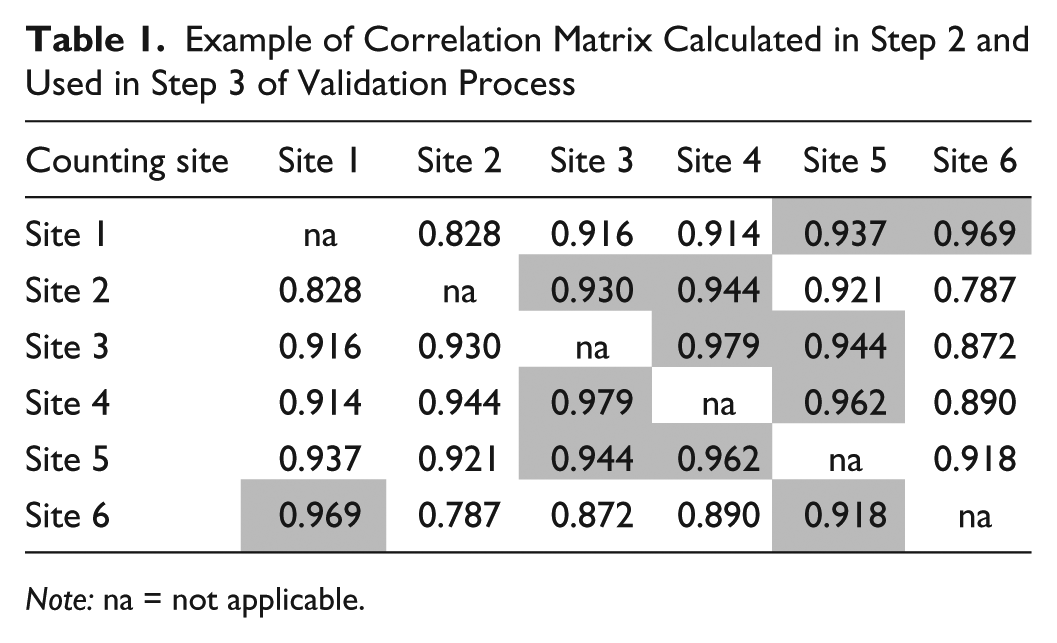
Note: na = not applicable.

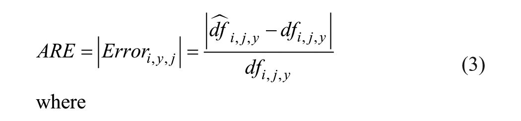
Error Measurement

The accuracy of a daily factor estimation is defined by the absolute relative error (ARE) as given in Equation 3. The flagged daily factors are removed and estimated through interpolation. The ARE of each daily factor interpolation is reported in the Results and Discussion section.

\begin{array}{l} A R E = | E r r o r_{i, y, j} | = \frac{| {\hat{d f}}_{i, j, y} - d f_{i, j, y} |}{d f_{i, j, y}} \\ where \end{array}

$| E r r o r_{i, y, j} |$ = the ARE for reference bicycle counting site i, based on the estimated and observed daily factors on day j of cycling season y,

${\hat{d f}}_{i, y, j}$ = the estimated daily factor for reference site i on day j of cycling season y,

$d f_{i, y, j}$ = the observed daily factor for reference site i on day j of cycling season y.

Data

The continuous bicycle count dataset used in this analysis was obtained from inductive loop bicycle counters manufactured by Eco-Counter and owned by Arlington County. Data from this equipment has been used in a wide range of studies and, when operating properly, ARE of these counters has been shown to be below 4% ( 2 , 23 – 25 ).

The data used to test the methods developed in this study came from 16 long-term bicycle counters in Arlington. The bicycle demand data in the analysis includes both weekday and weekend data for the 2015 and 2016 cycling seasons. The cycling season, which was defined in this study as all months where the cycling demand was at least 50% of the peak season demand, is from April 1 to November 30 in Arlington. Counting sites were only considered for the study if the AADB was greater than 250. Four counters in the Arlington dataset were disqualified from analysis for not satisfying that condition, bringing the number of eligible counters down to 16 from 20. The choice of cycling season months, with a threshold of 50% retention rate of the peak-demand month, and the minimum AADB condition were chosen to ensure that the daily bicycle counts at each counting site were large enough for validation purposes. As bicycle counts decrease, the proposed filtering method becomes less effective as the relative temporal variation in counts tends to rise rapidly. These two conditions represent limitations on when and where the filtering method can be applied.

Data Preparation

The automated validation and interpolation process has two stages. In the first stage, the data is scanned for extended periods of zero counts or missing data. The validation and interpolation program includes a parameter: the zero or missing data threshold. If a counting site has missing or zero data for more days than the threshold permits, then that counting site is removed from analysis. The threshold was set at 15 days in this study. This threshold was selected to agree with the corr_min value described in the Methodology section. If a counting site has more than 15 days of missing or zero data in a year, then the correlation of daily factors with other counting sites is not high enough for validation purposes. In the second stage, the ratio of daily factors for each counting site to the daily factors of the two closest references, as explained in Step 3 of the Methodology section, are taken to flag any days with anomalous bicycle counts. Each counting site in the analysis was validated and interpolated prior to testing the process with anomaly simulations. The first stage of the process removed two counters from analysis in 2015 and one in 2016. In the second stage seven and eight counter-days were flagged and interpolated in 2015 and 2016 respectively.

Simulation of Zero and Reduced Data

Once the data was prepared, by initially running the two stages of the validation and interpolation process, counting data was altered from the dataset to simulate anomalies in the bicycle counting data. For each bike season, 25 data anomalies were randomly created. For each anomaly, a counting site and date during the cycling season were randomly selected. Then, an anomaly duration was randomly chosen from the following possibilities: 6 hours (7:00 a.m. to 1:00 p.m.), 12 hours (7:00 a.m. to 7:00 p.m.), 1 day, 2 days, and 5 days. For the Arlington data, a total of 64 days of data anomalies were randomly selected for 2015, of which four were 6 hours’ duration, five were 12 hours and 55 were full-day anomalies. In 2016, a total of 45 days of data anomalies were randomly selected, of which six were 6 hours, six were 12 hours and 33 were full days.

Three separate trials were performed. In the first trial, anomalies were created by replacing ground truth hourly counts with zero values for the duration of each anomaly. This situation represents either a complete blockage of the bicycle facility, or an automatic counter going offline. In the second and third trials, the hourly counts were reduced to 25% and 40% of the ground truth values, respectively, for the same randomly chosen counters, dates, and durations. The second and third trials represent situations that diminish but do not reduce bicycle counts to zero, such as construction projects near bicycle facilities, or partial blockages of a bicycle facility at the counting site location.

Results and Discussion

The data validation process is highly effective at filtering out days with significantly reduced bicycle count anomalies. Table 2 shows a summary, by counting site and by year, of all the days reduced to zero and 25% of the measured bicycle counts, and the proportion of those days that were subsequently flagged and interpolated. When combining the 2 years of analysis, 113 counter-days were simulated to have anomalous data in Arlington, of which, 98 days were flagged and interpolated in both the first (zero data) and second (25% of the measured bicycle counts) trials. None of the 10 days with only 6 hours of anomalous data were flagged, 10 out of 11 days with 12 hours of anomalous data were flagged and interpolated, and 88 out of 92 days with the entire day of anomalous data were flagged and interpolated. The days with 6 hours of anomalous data were not flagged because the daily factor was not decreased sufficiently to be triggered in Step 5 of the validation procedure. Had a lower e value been used, more of these days would have been flagged; however, it would have come at the cost of false positives due to inherent variation in daily factors between sites. Most (91%) of the days with 12 hours of anomalous data were flagged and interpolated because they had a more substantial decrease in their daily factor. Almost all (96%) of the full days of anomalous data were flagged and interpolated. There were four full days of anomalous data that were not flagged (at the Roosevelt Bridge counting site in 2015) because one of the two reference sites had anomalous data over the same period. This result exposes one of the vulnerabilities of the process in detecting zero or reduced data; if multiple counting sites have periods of zero or reduced data simultaneously, the ability of the process to identify those anomalies is diminished. However, a well-maintained set of long-term counters is not likely to have multiple counting sites offline over the same period. The trials in this study introduced considerably more anomalies to the set of counting sites than what was typically observed in the bicycle counting data.

Table 2.

Results from Automated Validation of Data Anomaly Simulations

	2015				2016
Arlington counting site	AADB	Anomalies/flagged			AADB	Anomalies/flagged
Arlington counting site	AADB	6 h	12 h	Full day	AADB	6 h	12 h	Full day
Trials 1 and 2: reduced to 0% and 25% of ground truth
14th Street Bridge	1739			10/10	1896			5/5
Arlington Mill Drive Trail	350	NA			354			7/7
Ballston Connector	288			14/14	291			5/5
Bikeometer	1246			5/5	1302			3/3
Bluemont Connector	199			7/7	208	NA
CC Connector	689		1/1		722	0 /1
Custis Bon Air	1009				1026		1/1	4/4
Custis Rosslyn	1321		1/1		1434	0/1
Key Bridge	1955				1943	0/1
MVT Airport South	2155				2125		2/2
Roosevelt Bridge	398			5/9	445		1/1	2/2
TR Island	1332	0/1			1308	0/1
WOD Bon Air East	1014	0/1	0/1	3/3	968	0/1	1/1	1/1
WOD Bon Air West	1504	0/1	1/1	5/5	1484
WOD Columbia Pike	846	0/1	1/1	6/6	805	0/1	1/1	6/6
WOD East Falls Church	750	NA			1116
Total		0/4	4/5	55/59		0/6	6/6	33/33
Trial 3: reduced to 40% of ground truth
14th Street Bridge	1739			10/10	1896			5/5
Arlington Mill Drive Trail	350	NA			354			7/7
Ballston Connector	288			14/14	291			4/5
Bikeometer	1246			5/5	1302			1/3
Bluemont Connector	199			7/7	208	NA
CC Connector	689		1/1		722	0/1
Custis Bon Air	1009				1026		0/1	4/4
Custis Rosslyn	1321		0/1		1434	0/1
Key Bridge	1955				1943	0/1
MVT Airport South	2155				2125		0/2
Roosevelt Bridge	398			5/9	445		1/1	2/2
TR Island	1332	0/1			1308	0/1
WOD Bon Air East	1014	0/1	0/1	3/3	968	0/1	1/1	1/1
WOD Bon Air West	1504	0/1	0/1	5/5	1484
WOD Columbia Pike	846	0/1	1/1	5/6	805	0/1	1/1	6/6
WOD East Falls Church	750	NA			1116
Total		0/4	2/5	54/59		0/6	3/6	30/33

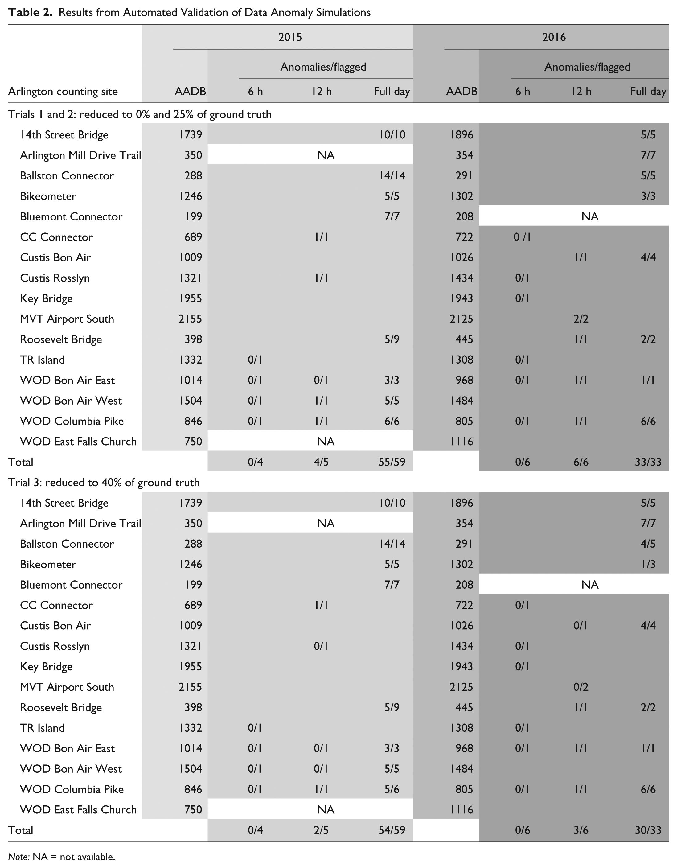
Note: NA = not available.

The results from the third trial, in which bicycle counts were reduced to 40% of the measured bicycle counts for the duration of the simulated anomaly, are also presented in Table 2. The results indicate that an anomaly causing bicycle counts to reduce to 40% of ground truth counts is likely to be detected by the validation program only if the anomaly persists for most of the day. A total of 89 days of anomalous data were flagged, compared with 98 days in the first and second trials. None of the 10 days with only 6 hours of anomalous data were flagged, which was unchanged from the first and second trials. The process did not perform as well in cases with 12 hours of anomalous data in the third trial compared with the first two; only 5 out of 11 days were flagged and interpolated. Although most (84 out of 92 days) anomalies spanning an entire day were flagged and interpolated, the results were inferior when compared with the first two trials. Four full days of anomalous data were not flagged by the process that had been flagged in the first two trials. These results are in concert with the theoretical limits of the process. If the parameter e is set at 2, as it was in all three trials, then the filtering process is not likely to detect anomalies that reduce bicycle counts by less than half of the daily total.

In cases where the anomaly was flagged, a daily factor was then interpolated by averaging the daily factor of the two most similar reference counting sites. Table 3 presents the anomalous daily factors for all three trials, the interpolated daily factors in the first (zero-data) trial and the ground truth factors for each of the 98 days that were flagged in the first and second trials. On average, the interpolated daily factor in the first and second trial had an ARE of 9.5% when compared with the ground truth; the third trial had a ARE of 10.2%. Note that 9 days have missing anomalous daily factors in the third trial because those days were not flagged in that trial. The distribution of ARE values is shown in Figure 2, illustrating that most of the 98 interpolated daily factors had an ARE <10%. For illustrative purposes, the daily factors for the counting site known as Ballston Connector, for 2015 are shown in Figure 3. The green trendline shows the ground truth daily factors. The red triangles represent the 14 days of anomalies simulated in the first trial, blue squares in the second trial, and orange circles in the third trial. The black diamonds represent the interpolated daily factors for the same 14 days in the first trial. The interpolated daily factors follow the ground truth factors closely. The ARE of the 14 days ranged from 1% to 16%. Note that the interpolated daily factors varied slightly when comparing the first two trials with the third trial. In several cases, a counting site with multiple days of anomalies would be assigned a different reference in the third trial when compared with the first two trials, which could result in slightly differing interpolated daily factors. To conserve space, the interpolated daily factors in figures 2 and 3 and Table 3 are only included for the first trial.

Table 3.

Reduced, Interpolated and Ground Truth Daily Factors for Three Data Anomaly Trials

Date	Counting site	Daily factor for zero anomaly Trial 1	Daily factor for 25% anomaly Trial 2	Daily factor for 40% anomaly Trial 3	Interpolated factor for zero anomalyTrial 1	Factor (ground truth)	ARE (%) for zero anomaly Trial 1
15-07-16	14th Street Bridge	0.000	0.410	0.652	1.467	1.588	8%
15-07-17	14th Street Bridge	0.000	0.310	0.489	1.169	1.194	2%
15-07-18	14th Street Bridge	0.000	0.180	0.282	0.832	0.691	21%
15-07-19	14th Street Bridge	0.000	0.200	0.315	0.835	0.768	9%
15-07-20	14th Street Bridge	0.000	0.296	0.468	1.045	1.141	8%
15-09-10	14th Street Bridge	0.000	0.201	0.320	0.755	0.777	3%
15-09-11	14th Street Bridge	0.000	0.341	0.540	1.350	1.315	3%
15-09-12	14th Street Bridge	0.000	0.067	0.106	0.563	0.259	117%
15-09-13	14th Street Bridge	0.000	0.248	0.391	1.205	0.956	26%
15-09-14	14th Street Bridge	0.000	0.345	0.544	1.345	1.331	1%
15-04-02	Ballston Connector	0.000	0.314	0.471	1.044	1.144	9%
15-06-21	Ballston Connector	0.000	0.245	0.370	1.000	0.894	12%
15-08-01	Ballston Connector	0.000	0.300	0.464	1.133	1.106	2%
15-08-02	Ballston Connector	0.000	0.260	0.406	1.134	0.988	15%
15-08-03	Ballston Connector	0.000	0.311	0.482	1.160	1.158	0%
15-08-04	Ballston Connector	0.000	0.340	0.529	1.221	1.270	4%
15-08-05	Ballston Connector	0.000	0.322	0.496	1.247	1.207	3%
15-09-06	Ballston Connector	0.000	0.274	0.420	1.198	1.005	19%
15-09-07	Ballston Connector	0.000	0.333	0.514	1.151	1.249	8%
15-09-08	Ballston Connector	0.000	0.318	0.493	1.198	1.190	1%
15-09-09	Ballston Connector	0.000	0.311	0.486	1.273	1.151	11%
15-09-10	Ballston Connector	0.000	0.234	0.359	0.843	0.859	2%
15-11-23	Ballston Connector	0.000	0.179	0.279	0.691	0.685	1%
15-11-24	Ballston Connector	0.000	0.190	0.290	0.712	0.692	3%
15-04-17	Bluemont Connect.	0.000	0.247	0.385	1.013	0.919	10%
15-04-18	Bluemont Connect.	0.000	0.361	0.544	1.341	1.331	1%
15-07-12	Bluemont Connect.	0.000	0.340	0.523	1.205	1.306	8%
15-07-13	Bluemont Connect.	0.000	0.247	0.359	0.844	0.879	4%
15-07-14	Bluemont Connect.	0.000	0.309	0.477	1.129	1.180	4%
15-07-15	Bluemont Connect.	0.000	0.304	0.472	1.158	1.145	1%
15-07-16	Bluemont Connect.	0.000	0.381	0.605	1.428	1.512	6%
15-09-30	CC Connector	0.128	0.285	0.372	0.837	0.742	13%
15-07-10	Custis Rosslyn	0.190	0.461		1.269	1.266	0%
15-04-21	Roosevelt Bridge	0.000	0.356	0.562	1.258	1.368	8%
15-04-22	Roosevelt Bridge	0.000	0.256	0.390	0.863	0.969	11%
15-05-11	Roosevelt Bridge	0.000	0.418	0.655	1.390	1.611	14%
15-05-12	Roosevelt Bridge	0.000	0.385	0.606	1.414	1.481	4%
15-11-17	Roosevelt Bridge	0.000	0.279	0.431	0.988	1.064	7%
15-04-04	WOD Bon Air East	0.000	0.148	0.233	0.540	0.577	6%
15-04-05	WOD Bon Air East	0.000	0.339	0.536	1.150	1.333	14%
15-08-21	WOD Bon Air East	0.000	0.302	0.481	1.220	1.194	2%
15-04-07	WOD Bon Air West	0.000	0.170	0.267	0.645	0.663	3%
15-04-08	WOD Bon Air West	0.000	0.109	0.171	0.428	0.423	1%
15-04-09	WOD Bon Air West	0.000	0.096	0.150	0.440	0.373	18%
15-04-10	WOD Bon Air West	0.000	0.102	0.159	0.433	0.396	9%
15-04-11	WOD Bon Air West	0.000	0.348	0.555	1.358	1.373	1%
15-11-17	WOD Bon Air West	0.096	0.246		0.778	0.681	14%
15-06-30	WOD Columbia Pike	0.000	0.260	0.410	1.113	1.009	10%
15-07-01	WOD Columbia Pike	0.000	0.236	0.371	0.993	0.912	9%
15-07-02	WOD Columbia Pike	0.000	0.173	0.272	0.694	0.672	3%
15-07-03	WOD Columbia Pike	0.000	0.470		1.800	1.823	1%
15-07-04	WOD Columbia Pike	0.000	0.167	0.259	0.748	0.639	17%
15-07-11	WOD Columbia Pike	0.000	0.375	0.593	1.373	1.458	6%
15-09-22	WOD Columbia Pike	0.113	0.315	0.434	0.990	0.902	10%
15-11-18	Bikeometer	0.000	0.209	0.328	0.934	0.815	15%
15-11-19	Bikeometer	0.000	0.089	0.135	0.436	0.339	29%
15-11-20	Bikeometer	0.000	0.204	0.322	0.827	0.797	4%
15-11-21	Bikeometer	0.000	0.133	0.206	0.525	0.513	2%
15-11-22	Bikeometer	0.000	0.065	0.103	0.332	0.258	29%
16-05-03	14th Street Bridge	0.000	0.153	0.243	0.645	0.604	7%
16-05-04	14th Street Bridge	0.000	0.201	0.316	0.774	0.786	2%
16-05-05	14th Street Bridge	0.000	0.184	0.289	0.708	0.717	1%
16-05-06	14th Street Bridge	0.000	0.055	0.087	0.262	0.216	21%
16-05-07	14th Street Bridge	0.000	0.152	0.241	0.663	0.600	11%
16-09-21	Arlington Mill Drive	0.000	0.304	0.481	1.207	1.173	3%
16-09-22	Arlington Mill Drive	0.000	0.273	0.421	1.279	1.049	22%
16-10-08	Arlington Mill Drive	0.000	0.045	0.063	0.15	0.180	17%
16-10-09	Arlington Mill Drive	0.000	0.149	0.237	0.684	0.581	18%
16-10-10	Arlington Mill Drive	0.000	0.264	0.409	1.034	1.029	0%
16-10-11	Arlington Mill Drive	0.000	0.215	0.335	0.897	0.840	7%
16-10-12	Arlington Mill Drive	0.000	0.270	0.418	1.059	1.015	4%
16-09-02	Ballston Connector	0.000	0.319	0.500	1.247	1.239	1%
16-09-03	Ballston Connector	0.000	0.249		0.874	0.933	6%
16-09-04	Ballston Connector	0.000	0.302	0.479	1	1.191	16%
16-09-05	Ballston Connector	0.000	0.302	0.465	1.157	1.160	0%
16-09-06	Ballston Connector	0.000	0.344	0.535	1.432	1.321	8%
16-05-13	Custis Bon Air	0.000	0.165	0.262	0.651	0.649	0%
16-05-14	Custis Bon Air	0.000	0.243	0.385	1.022	0.952	7%
16-09-20	Custis Bon Air	0.183	0.468		1.198	1.289	7%
16-11-02	Custis Bon Air	0.000	0.323	0.510	1.154	1.262	9%
16-11-03	Custis Bon Air	0.000	0.218	0.343	0.797	0.851	6%
16-07-09	MVT Airport South	0.146	0.452		1.285	1.359	5%
16-08-05	MVT Airport South	0.198	0.418		1.095	1.068	3%
16-10-27	Roosevelt Bridge	0.000	0.213	0.328	0.737	0.820	10%
16-10-28	Roosevelt Bridge	0.000	0.251	0.384	0.887	0.964	8%
16-11-26	Roosevelt Bridge	0.013	0.080	0.117	0.267	0.272	2%
16-05-17	WOD Bon Air East	0.056	0.087	0.099	0.227	0.165	37%
16-09-02	WOD Bon Air East	0.000	0.378	0.601	1.448	1.495	3%
16-04-03	WOD Columbia Pike	0.000	0.100	0.160	0.363	0.393	8%
16-04-04	WOD Columbia Pike	0.000	0.103	0.158	0.437	0.383	14%
16-04-05	WOD Columbia Pike	0.000	0.069	0.104	0.307	0.264	16%
16-04-06	WOD Columbia Pike	0.000	0.129	0.198	0.497	0.494	1%
16-04-07	WOD Columbia Pike	0.000	0.054	0.078	0.169	0.198	15%
16-09-30	WOD Columbia Pike	0.000	0.100	0.158	0.429	0.392	9%
16-11-18	WOD Columbia Pike	0.068	0.249	0.354	0.836	0.775	8%
16-04-17	Bikeometer	0.000	0.296		1.059	1.169	9%
16-04-18	Bikeometer	0.000	0.324		1.031	1.280	19%
16-09-28	Bikeometer	0.000	0.144	0.228	0.609	0.567	7%

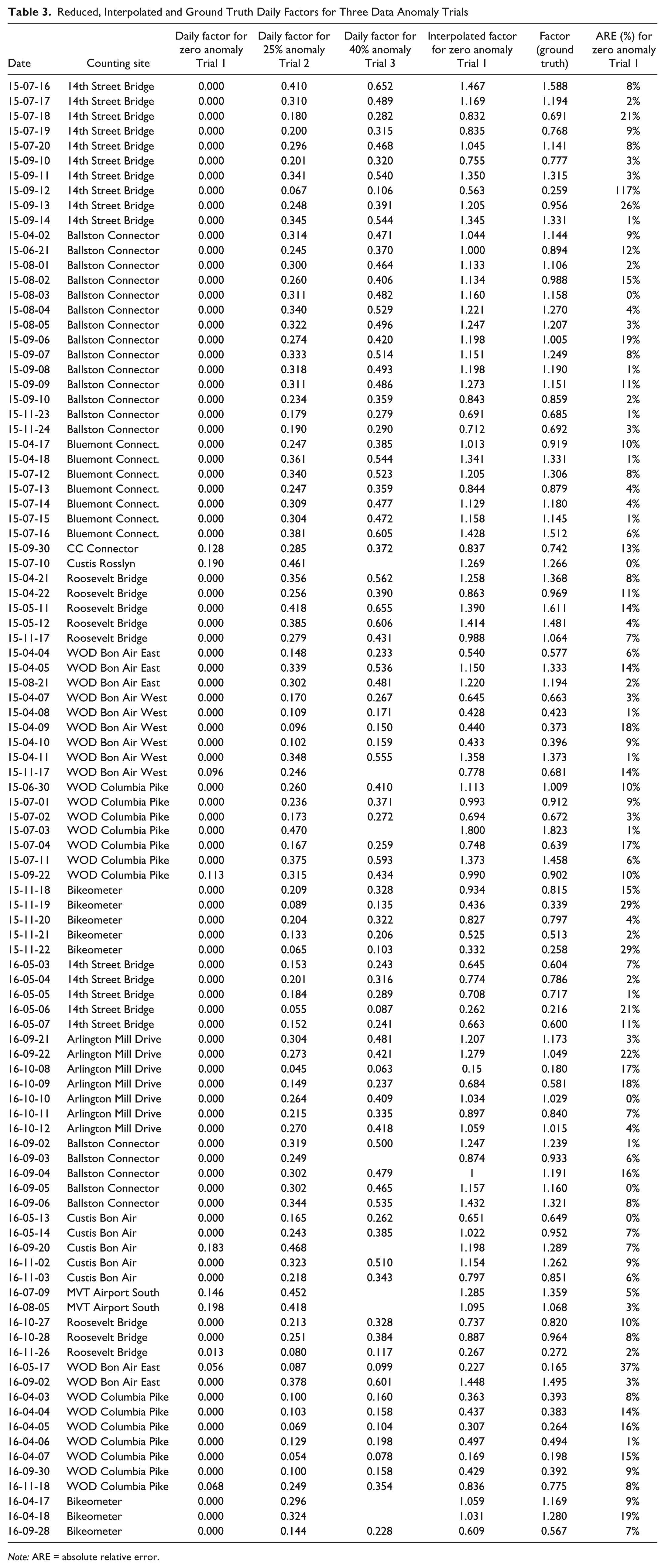
Note: ARE = absolute relative error.

Figure 1.

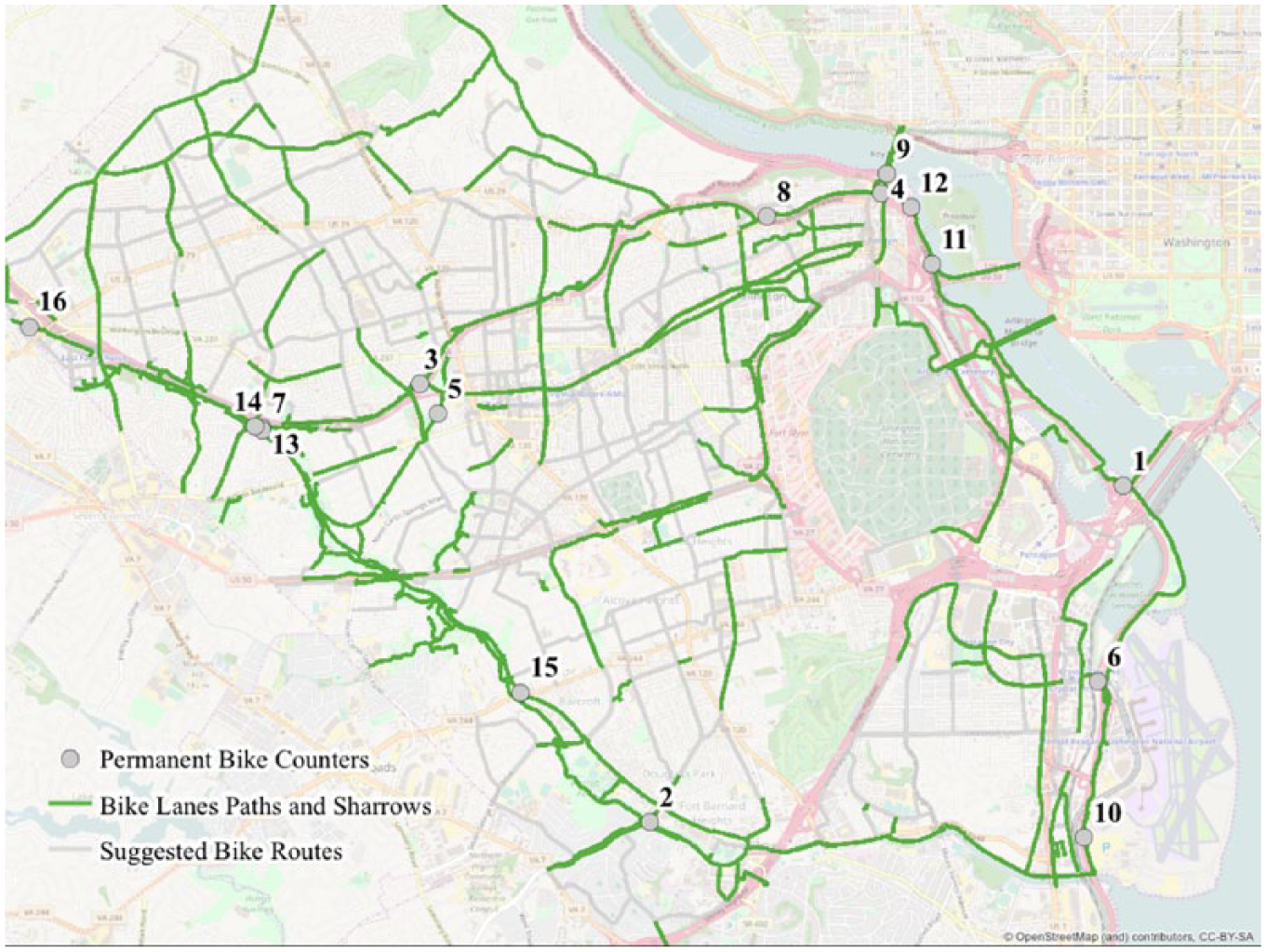
Long-term bicycle counters in Arlington, VA: 14th Street Bridge (1), Arlington Mill Drive Trail (2), Ballston Connector (3), Bikeometer (4), Bluemont Connector (5), CC Connector (6), Custis Bon Air (7), Custis Rosslyn (8), Key Bridge (9), MVT Airport South (10), Roosevelt Bridge (11), TR Island (12), WOD Bon Air East (13), WOD Bon Air West (14), WOD Columbia Pike (15), and WOD East Falls Church (16).

Figure 2.

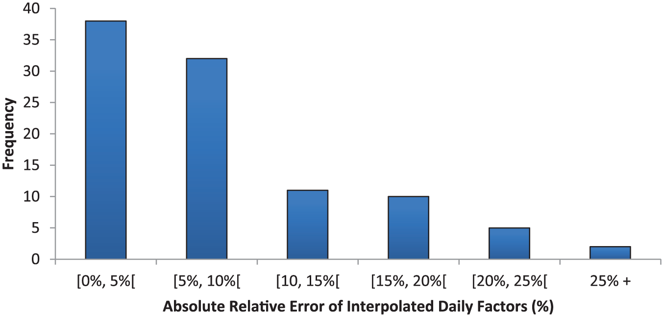
Frequency of ARE of interpolated daily factors for first trial, zero-anomaly simulations.

Figure 3.

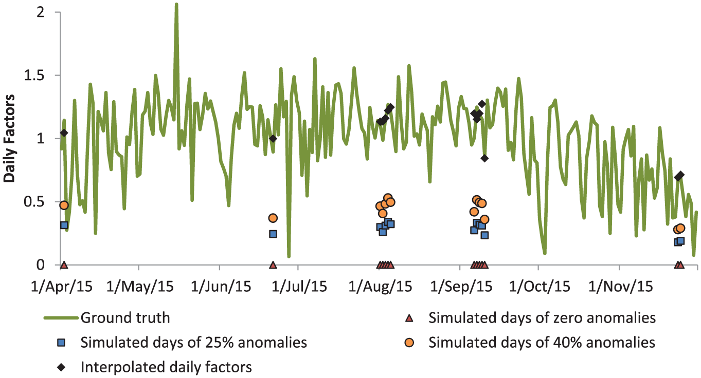
Example of interpolated daily factors after the automated data validation and interpolation process.

Conclusion

The accuracy of AADB estimation from short-term counts is highly sensitive to error in the reference data, particularly when the reference experiences significant undercounting during the short-term count period. An automated validation and interpolation process for reference bicycle count data would improve the quality of the reference data and, in the process, make AADB estimation from short-term counts more feasible in practice. This study proposed a methodology for grouping similar counting sites, validating the data by comparing daily factors of similar sites and interpolating any periods of anomalous data using the daily factors of the similar counting sites. The methodology was then tested on long-term bicycle count data from Arlington, with simulated anomalies. In three trials, data anomalies were artificially created that reduced counts to 0%, 25%, and 40%, respectively, of the measured bicycle counts for 6 consecutive hours, 12 consecutive hours, a full day, two consecutive full days, and five consecutive full days.

The days with 6 hours of anomalous data were not flagged in any of the three trials because the daily factors were not decreased sufficiently to be identified in the validation procedure. In the first and second trials, 91% of the days with 12 hours of anomalous data were flagged compared with 45% in the third trial. Similarly, in the first and second trials, 96% of full-day anomalies were flagged compared with 91% in the third trial. The third trial, in which hourly bicycle counts were reduced to 40% of measured values, approached the validation program limit. Given the parameters used in the study, if an anomaly does not reduce counts to below 50% of the ground truth daily total, then the validation program is not likely to flag the anomaly. When anomalies are flagged, the interpolated daily factors are close to the ground truth. Of the 98 anomalies flagged in the first and second trials, the AARE of the interpolated daily factor was 9.5%. Of the 89 anomalies flagged in the third trial, the AARE was 10.2%.

The proposed methodology, allowing for automatic validation and interpolation of reference bicycle count data, is part of a research project conducted in partnership with Eco-Counter. The methodology has been incorporated into software that will be accessible to jurisdictions with Eco-Counter equipment. However, the proposed methodology could be applied to continuous daily bicycle count data collected from any bicycle counting system and could be incorporated into other bicycle data archive and visualization tools. By applying this methodology, a transportation agency with multiple proximate reference counters could identify missing and erroneous data and subsequently interpolate to correct it. Two limitations of the proposed methodology must be highlighted. Firstly, an absolute minimum of three proximate reference counters are needed, thus this methodology is most applicable to bicycle counting sites across an urban center or region. Ideally, a transportation agency might have 10 or more reference counters across their jurisdiction to collect bicycle count data at several similar locations for each type of cycling facility present across the bicycle network. Secondly, in colder climates, this analysis is only appropriate during the cycling season. In this study, the cycling season was defined as all months with at least 50% of the cycling demand compared with the peak month. During the winter season, in many jurisdictions located in cold climatic zones, a combination of low cycling demand, high weather variability, and great variability in surface conditions across cycling facilities complicate the validation and interpolation process making an automated tool prone to error.

Future work will include testing the validation and interpolation tool developed in this paper with larger datasets and testing anomalies that result in increased bicycle counts. The logic behind the validation process could also be expanded to allow for more than two references to be used. The tool is intended to be the first stage of a larger program that estimates AADB from short-term counts. The program would receive both short-term counts and long-term reference counts as inputs. The program would then validate and interpolate reference data, cluster validated reference sites into similar groups, match short-term counts to reference clusters, estimate the quality of the short-term count, and finally estimate the AADB of the short-term counting site. By completely automating the process of data validation and AADB extrapolation of short-term counts, transportation agencies would find it more feasible to conduct comprehensive bicycle count programs that extend to hundreds of locations through a city or regional bike network. The outcome would help practitioners in bicycle infrastructure planning, and in evaluating injury risk across the network.

Footnotes

Acknowledgements

Funding for this project was provided in part by the Natural Sciences and Engineering Research Council and Eco-Counter. We thank Arlington County for access to their bicycle counting data.

Author Contributions

The authors confirm contribution to the paper as follows: study conception and design: DB; data collection: Eco-Counter, Arlington County; analysis and interpretation of results: DB, SM, FM, LM-M; draft manuscript preparation: DB. All authors reviewed the results and approved the final version of the manuscript.

The Standing Committee on Highway Traffic Monitoring (ABJ35) peer-reviewed this paper (18-04717).

References

Fournier

Christofa

Knodler

M. A.

A Mixed Methods Investigation of Bicycle Exposure in Crash Rates. Accident Analysis & Prevention, March 1, 2017.

Nosal

Miranda-Moreno

L. F.

Cycling and Weather: A Multi-City and Multi-Facility Study in North America. Presented at 91st Annual Meeting of theTransportation Research Board, Washington, D.C., 2012.

Nordback

Marshall

W. E.

Janson

B. N.

Stolz

Estimating Annual Average Daily Bicyclists: Error and Accuracy. Transportation Research Record: Journal of the Transportation Research Board, 2013. 2339: 90–97.

Nosal

Miranda-Moreno

L. F.

The Effect of Weather on the Use of North American Bicycle Facilities: A Multi-City Analysis Using Automatic Counts. Transportation Research Part A: Policy and Practice, Vol. 66, No. 1, 2014. 213–225.

Beitel

McNee

Miranda-Moreno

L. F.

Quality Measure of Short-Duration Bicycle Counts. Transportation Research Record: Journal of the Transportation Research Board, 2017. 2644: 64–71.

Beitel

Miranda-Moreno

Methods for Improving and Automating the Estimation of Average Annual Daily Bicyclists. Presented at 95th Annual Meeting of the Transportation Research Board, Washington, D.C., 2016.

Miranda-Moreno

L. F.

Nosal

Schneider

R. J.

Proulx

Classification of Bicycle Traffic Patterns in Five North American Cities. Transportation Research Record: Journal of the Transportation Research Board, 2013. 2339: 68–79.

Nosal

Miranda-Moreno

L. F.

Krstulic

Incorporating Weather: A Comparative Analysis of Average Annual Daily Bicyclist Estimation Methods. Presented at 93rd Annual Meeting of the Transportation Research Board, Washington, D.C., 2014.

Hankey

Lindsey

Marshall

Day-of-Year Scaling Factors and Design Considerations for Nonmotorized Traffic Monitoring Programs. Transportation Research Record: Journal of the Transportation Research Board, 2014. 2468: 64–73.

10.

Figliozzi

Johnson

Monsere

Nordback

Methodology to Characterize Ideal Short-Term Counting Conditions and Improve AADT Estimation Accuracy Using a Regression-Based Correcting Function. Journal of Transportation Engineering, Vol. 140, No. 5, 2014, p. 04014014.

11.

El Esawey

Mosa

A. I.

Determination and Application of Standard K Factors for Bicycle Traffic. Transportation Research Record: Journal of the Transportation Research Board, 2015. 2527: 58–68.

12.

El Esawey

Lim

Sayed

Mosa

A. I.

Development of Daily Adjustment Factors for Bicycle Traffic. Journal of Transportation Engineering, Vol. 139, No. 8, 2013. 859–871.

13.

El Esawey

. Estimation of Annual Average Daily Bicycle Traffic with Adjustment Factors. Transportation Research Record: Journal of the Transportation Research Board, 2014. 2443: 106–114.

14.

El Esawey

Toward a Better Estimation of Annual Average Daily Bicycle Traffic: Comparison of Methods for Calculating Daily Adjustment Factors. Transportation Research Record: Journal of the Transportation Research Board, 2016. 2593: 28–36.

15.

Nosal

Improving the Accuracy of Bicycle AADT Estimation: Temporal Patterns, Weather and Bicycle AADT Estimation Methods. Masters degree thesis. Civil Engineering and Applied Mechanics, McGill University, Montreal, 2014.

16.

Fournier

Christofa

Knodler

M. A.

A Sinusoidal Model for Seasonal Bicycle Demand Estimation. Transportation Research Part D: Transport and Environment, Vol. 50, 2017. 154–169.

17.

Lindsey

. The Minnesota Bicycle and Pedestrian Counting Initiative: Implementation Study. Minnestoa Department of Transportation, St. Paul, MN, 2015.

18.

Jackson

K. N.

Stolz

Cunningham

Nonmotorized Site Selection Methods for Continuous and Short-Duration Volume Counting. Transportation Research Record: Journal of the Transportation Research Board, 2015. 2527: 49–57.

19.

FHWA. Traffic Monitoring Guide. U.S. Department of Transportation, Federal Highway Administration, Washington, D.C., 2013.

20.

Jackson

K. N.

O’Brien

S. W.

Searcy

S. E.

Warchol

S. E.

Quality Assurance and Quality Control Processes for a Large-Scale Bicycle and Pedestrian Volume Data Program. Transportation Research Record: Journal of the Transportation Research Board, 2017. 2644: 19–29.

21.

TRB. Guidebook on Pedestrian and Bicycle Volume Data Collection. The National Academies Press, Washington, D.C., 2014.

22.

Nordback

Tufte

McNeil

Harvey

Watkins

Bike-Ped Portal: Development of an Online Nonmotorized Traffic Count Archive. National Institute for Transportation and Communities (NITC), Portland, OR, 2017.

23.

Miranda-Moreno

Nosal

Weather or Not to Cycle. Transportation Research Record: Journal of the Transportation Research Board, 2011. 2247: 42–52.

24.

Nordback

Piatkowski

Janson

B. N.

Marshall

W. E.

Krizek

K. J.

Main

D. S.

Using Inductive Loops to Count Bicycles in Mixed Traffic. Journal of Transportation of the Institute of Transportation Engineers, Vol. 2, No. 1. 39–56, 2011.

25.

Nordback

Janson

Automated Bicycle Counts: Lessons from Boulder, Colorado. Transportation Research Record: Journal of the Transportation Research Board, 2010. 2190: 11–18.