Fuel Consumption Optimization Model for the Multi-Period Inventory Routing Problem

Abstract

In the traditional multi-period inventory routing problem (MIRP), traveling distance is considered as the only measurement of vehicles’ variable transportation cost; however, it is in fact the fuel consumption cost, not the distance, which is the greater concern. This paper evaluates vehicles’ variable transportation cost by fuel consumption, which is influenced by distance, load, and fuel price. It presents an integer program to formally characterize the fuel consumption considered MIRP (FCMIRP), which can help enterprises obtain a more accurate tradeoff between transportation and inventory costs. It also benefits the environment, because reducing fuel consumption will curb carbon dioxide (CO₂) emissions. Valid inequalities are added to strengthen the model and use a branch-and-cut algorithm. Computational tests indicate that the FCMIRP can decrease fuel consumption and total cost over the traditional model. Factors that influence the results of FCMIRP are also discussed.

With growing energy shortages and rising prices, governments and enterprises have begun to pay close attention to sustainable development, to save energy and protect the environment. For example, the U.S. government has made energy policies to reduce fossil fuel consumption ( 1 ). The United Nations and the European Union have enacted legislation to control energy consumption. Companies like Wal-Mart and IKEA have started to invest in renewable energy, hoping to decrease traditional energy (petroleum or coal) consumption.

Supply chain activities, such as production, transportation, and inventory, all consume energy. Therefore, in recent years, researchers have begun to consider energy consumption in the supply chain ( 2 ). Among all the logistics activities, transportation is regarded as one of the largest consumers of petroleum ( 3 ). Thus, reducing fuel consumption in transportation will contribute to green logistics and cost reduction.

Generally, transportation costs are divided into two parts: (i) fixed cost, including driver wages, vehicle maintenance and depreciation, and so on; and (ii) variable cost, which mainly refers to fuel cost ( 4 ). Therefore, accurate computation of transportation cost can help plan more practical vehicle routes. Because fuel cost is related to many factors (distance, load, road condition, speed, etc.) ( 2 , 4 ), it is not accurate to consider travel distance alone. For example, the fuel consumption of a fully loaded vehicle is always greater than an identical but empty vehicle when they are traveling along a specific route at the same speed.

Up to now, many studies on inventory routing problems (IRPs) have used distance as the sole measurement of variable transportation cost. Because in IRPs there is a tradeoff to be made between transportation and inventory costs, if the computation of transportation cost is inaccurate, it will not only lead to suboptimal traveling schedules, but will also fail to achieve exact inventory strategies. Therefore, in this paper fuel cost is used as vehicles’ variable transportation cost. It is worth mentioning that considering fuel consumption in MIRP also benefits the environment, because transportation is logistics’ largest source of CO₂ emissions ( 5 ), which are caused by fuel consumption.

To conclude, this study makes the following contributions:

As far as is known, this paper is among the first to examine the influence of fuel cost on MIRP in detail.

Numerical experiments demonstrate that FCMIRP can reduce overall cost and achieve a better environmental benefit. This could provide managerial insights for enterprises and governments in green logistics.

The remainder of the paper is organized as follows. Section 2 reviews related literature. Section 3 presents mathematical models for the FCMIRP and the traditional MIRP. Section 4 describes the solution method, and Section 5 presents numerical results. Conclusions follow in Section 6.

Literature Review

The IRP is a classic combinatorial optimization problem which determines simultaneously the optimal inventory strategy and vehicle schedules to minimize the supply chain’s total cost. IRP has been extensively studied since its introduction in ( 6 ). By considering different industrial applications and constraints, various types of IRPs have been formulated. For industrial applications, IRPs are classified as road-based IRPs or maritime IRPs. As to constraints, IRPs can be defined according to the following criteria: time horizon, supply chain topology, routing component, inventory policy, and fleet composition and size ( 7 ). For more details on IRPs see ( 7 , 8 ).

In a MIRP, the total cost is minimized by determining retailers’ optimal replenishment time and vehicle routes. ( 9 ) addresses a single period model which schedules multi-item replenishment with uncertain demand. ( 10 ) considers a many-to-one distribution network with multi-supplier and multi-product. ( 11 ) studies a multi-product multi-vehicle MIRP. There are also extensive studies on the algorithm for solving MIRP. The first type is the exact algorithm, including the branch-and-cut (B&C) algorithm and the branch-price-and-cut (BPC) algorithm. ( 12 ) develops the first B&C algorithm: in that paper, only one vehicle is available for each period. ( 13 ) uses the B&C algorithm for several classes of MIRPs: multi-vehicle MIRPs with homogeneous and heterogeneous vehicles, MIRPs with transshipment options, and MIRPs with added consistency features. ( 14 ) uses a BPC algorithm to solve a one-to-many MIRP with maximum-level (ML) inventory replenishment policy. Under an ML policy, any quantity of products can be delivered to a retailer as long as the retailer’s maximal inventory capacity is respected. The MIRP subsumes a vehicle routing problem (VRP) which is NP-hard, so (meta)heuristics are developed, including Variable Neighborhood Search ( 15 ), Tabu Search ( 16 ), Genetic Algorithm ( 10 ), and so on.

With increasing environmental pressures, researchers have started to consider fuel consumption and CO₂ emissions in the supply chain. ( 17 , 18 ) summarize recent models for sustainable supply chain management (SSCM). In SSCM, one of the most extensively studied areas is green VRP which explicitly includes fuel or emission cost in VRP models. ( 2 ) addresses a capacitated VRP that minimizes fuel consumption. ( 19 ) explores cumulative VRP, in which both distance and vehicle load are considered for calculating fuel consumption. ( 20 ) compares different objective functions for VRP to quantify their influence on cost and emissions, including minimizing comprehensive cost, minimizing travel distance, minimizing weighted load, and minimizing energy consumption. ( 21 ) extends the traditional heterogeneous VRP objective to include fuel and emission costs, and analyzes their influences. ( 22 ) proposes to consider CO₂ emissions in the facility location problem and suggests the difference between cost-minimization solutions and emission-minimization solutions. For detailed reviews of green logistics see ( 1 , 23 ).

Problem Formulation

In this section, the mathematical models for the FCMIRP and the traditional MIRP are presented.

Problem Description

Consider an outbound product distribution system consisting of a supplier and $N$ geographically dispersed retailers. In each period, vehicles depart from the supplier to distribute products to the retailers. Assumptions include:

The supplier only offers one type of product. At the beginning of each period, products are ready for distribution.

Vehicle routes start and end at the supplier, and can be completed in one time period.

Waiting, loading, and unloading times at each vertex are not considered.

Vehicles are homogeneous and capacitated.

Split delivery is not allowed: a retailer is visited by at most one vehicle in each period.

Retailers’ demands are deterministic but variable over periods. Their demands must be fulfilled; therefore, backorders are not allowed.

Retailers’ inventory capacities are limited, and the ML replenishment policy is applied.

Inventory holding costs are considered for both the supplier and the retailers. At the beginning of the time horizon, the initial inventory levels at each vertex are known.

The proposed FCMIRP uses the following notations:

Sets

$V = {0, 1, \dots, N}$ A set of all vertices, $i, j \in V$ ; vertex 0 is the supplier

$V' = {1, 2, \dots N}$ A set of retailers

$T =$ { $1, 2, \dots p$ } Time horizon, $t \in T$

Parameters

$d_{i}^{t}$ Retailer $i$ ’s demand in period $t$ (kg)

$c_{i j}$ Distance between vertex $i$ and vertex $j$ (km)

$Q$ The weight capacity of each vehicle (kg)

$h_{i}$ Inventory holding cost at vertex $i$ per unit weight per period ($/kg/period)

$I_{i}^{0}$ Initial inventory level of vertex $i$ at the beginning of the time horizon (kg)

$C_{i}$ Maximal inventory holding capacity at retailer $i$ (kg)

$r^{t}$ The product weight supplier receives (or produces) in period $t$ (kg)

$u$ Unit fuel price ($/L)

$u'$ Variable transportation cost per unit distance per vehicle ($/km)

$F$ Fixed vehicle cost per trip ($/trip)

$f_{d}$ Driver wage per hour ($/h)

$v$ Vehicle speed (km/h)

Decision variables

$x_{i j}^{t}$ $x_{i j}^{t} = 1$ if arc $(i, j)$ is traversed by a vehicle in period $t$ , otherwise 0

$a_{i j}^{t}$ The product weight carried by a vehicle through arc $(i, j)$ in period $t$ (kg)

$q_{i}^{t}$ The product weight delivered to retailer $i$ in period $t$ (kg)

$I_{i}^{t}$ The inventory level at vertex $i$ at the end of period $t$ (kg)

$ρ_{i j}^{t}$ Fuel consumption rate of each vehicle from vertex $i$ to vertex $j$ in period $t$ (L/km)

${F C}_{i j}^{t}$ Fuel cost of each vehicle from vertex $i$ to vertex $j$ in period $t$ ($)

Fuel Cost

The model proposed by ( 4 , 5 ) is used to compute fuel consumption. These papers state that fuel consumption mainly results from two elements: distance and fuel consumption rate (FCR)—fuel consumption per unit of distance, where FCR is linearly associated with a vehicle’s load according to statistical data. Some other complicated models for fuel calculation are also available. For example, it is possible to consider the effect of vehicle speed, road angle, acceleration, weather, and traffic condition. However, here a choice has been made to neglect some factors, based on the following reasons: (i) it is found that in many pieces of research the road angle and acceleration are set to 0 and the speed is assumed to be constant ( 21 , 24 , 25 ); (ii) it is impractical and unreasonable to attempt to quantify factors such as weather and traffic, because they vary significantly in different regions ( 5 ); (iii) IRP is a problem that is even more difficult than VRP, and it is necessary to keep the model tractable.

FCR is first formulated as

ρ_{i j}^{t} = ρ^{0} + \frac{ρ^{*} - ρ^{0}}{Q} a_{i j}^{t}

(1)

where $ρ^{0}$ , $ρ^{*}$ are the empty-load and full-load FCR respectively. As $ρ^{0}$ , $ρ^{*}$ and $Q$ are fixed for a specific type of vehicle, Equation 1 is simplified as

ρ_{i j}^{t} = ρ^{0} + β a_{i j}^{t}, in which β = \frac{ρ^{*} - ρ^{0}}{Q}

(2)

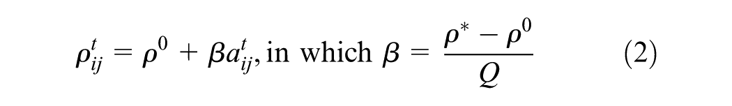
Therefore, the fuel cost from node $i$ to node $j$ in period $t$ is

{F C}_{i j}^{t} = u ρ_{i j}^{t} c_{i j} = u (ρ^{0} + β a_{i j}^{t}) c_{i j}

(3)

Mathematical Formulation

The completed formulation for FCMIRP is

\begin{matrix} Min f_{1} = \sum_{t \in T} \sum_{i \in V} h_{i} I_{i}^{t} + \sum_{t \in T} \sum_{j \in V'} {F x}_{0 j}^{t} + \sum_{t \in T} \sum_{i \in V} \sum_{j \in V} f_{d} c_{i j} x_{i j}^{t} / v \\ + \sum_{t \in T} \sum_{i \in V} \sum_{j \in V} u (ρ^{0} x_{i j}^{t} + β a_{i j}^{t}) c_{i j} \end{matrix}

(4)

subject to

I_{0}^{t} = I_{0}^{t - 1} + r^{t} - \sum_{i \in V'} q_{i}^{t} \forall t \in T

(5)

I_{i}^{t} = I_{i}^{t - 1} + q_{i}^{t} - d_{i}^{t} \forall i \in V', t \in T

(6)

I_{i}^{t} \geq 0 \forall i \in V, t \in T

(7)

I_{i}^{t} \leq C_{i} \forall i \in V', t \in T

(8)

q_{i}^{t} \leq C_{i} - I_{i}^{t - 1} \forall i \in V', t \in T

(9)

a_{i j}^{t} \leq {Q x}_{i j}^{t} \forall i \in V, \forall j \in V, t \in T

(10)

\sum_{j \in V} x_{i j}^{t} = \sum_{j \in V} x_{j i}^{t} \forall i \in V, t \in T

(11)

\sum_{j \in V} a_{i j}^{t} = \sum_{j \in V} a_{j i}^{t} - q_{i}^{t} \forall i \in V', i \neq j, t \in T

(12)

\sum_{j \in V} x_{j i}^{t} \leq 1 \forall i \in V', t \in T

(13)

x_{i i}^{t} = 0 \forall i \in V, t \in T

(14)

a_{i j}^{t} \geq 0 \forall i \in V, j \in V, t \in T

(15)

q_{i}^{t} \geq 0 \forall i \in V', t \in T

(16)

x_{i j}^{t} \in {0, 1} \forall i \in V, j \in V, t \in T

(17)

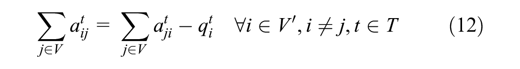
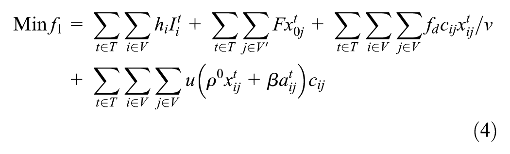
The objective function (4) minimizes the total cost, including inventory cost, fleet cost, driver wage, and fuel cost. Constraints (5) and (6) are the inventory balance equations at the supplier and the retailers respectively. Constraint (7) means that inventories cannot be negative at each vertex. Constraint (8) imposes maximal inventory level at retailers. Constraint (9) limits the product weight delivered to each retailer, to satisfy demand and to respect maximal inventory capacity. Constraint (10) guarantees that vehicles’ capacities are not violated. Constraint (11) indicates that the number of vehicles leaving a node is equal to that arriving at a node. Constraint (12) is the product flow balance equation at retailers and eliminates all subtours. Constraint (13) ensures that split delivery is not allowed. Constraints (14)–(17) define variable types.

For contrast, the mathematical formulation for traditional MIRPs is

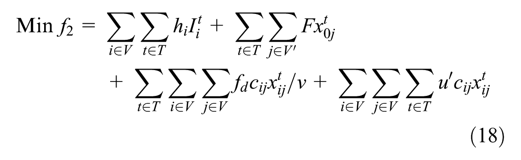
\begin{matrix} Min f_{2} = \sum_{i \in V} \sum_{t \in T} h_{i} I_{i}^{t} + \sum_{t \in T} \sum_{j \in V'} {F x}_{0 j}^{t} \\ + \sum_{t \in T} \sum_{i \in V} \sum_{j \in V} f_{d} c_{i j} x_{i j}^{t} / v + \sum_{i \in V} \sum_{j \in V} \sum_{t \in T} u' c_{i j} x_{i j}^{t} \end{matrix}

(18)

subject to (5)–(17) and

\sum_{i \in V'} q_{i}^{t} = \sum_{j \in V'} a_{0 j}^{t} \forall t \in T

(19)

Constraint (19) ensures that in each period the product weight delivered to all retailers is equal to that provided by the supplier. If this constraint is absented from the traditional model, sometimes a vehicle may carry more product (more than the weight delivered to all retailers) from the supplier, and then at the end of the trip the vehicle carries surplus product back to the supplier. However, these constraints are not necessary in FCMIRP, as vehicles will consume more fuel in such a scenario, which is not a wise choice for FCMIRP.

Valid Inequality and Solution Method

Valid Inequalities

( 11 , 12 , 26 ) have introduced several classes of valid inequalities for the IRPs. Some of them are extended to strengthen the models.

\sum_{j \in V} \sum_{l = 1}^{t} x_{j i}^{l} \geq (\sum_{l = 1}^{t - 1} d_{i}^{l} - I_{i}^{0}) / C_{i} \forall i \in V', \forall t \in T

(20)

Inequality (20) means that for retailer i, if its total demand over $[1, t - 1]$ is greater than its initial inventory level, then it has to be visited at least the number of times that corresponds to the right-hand side of the inequality in the interval $[1, t]$ .

Constraint (20) can be extended to any time interval $[t_{1}, t_{2}]$ ; consider that the maximal delivery weight takes the minimal value between a vehicle’s capacity and retailers’ inventory capacities. This yields inequality (21):

\begin{matrix} \sum_{j \in V} \sum_{t' = t_{1}}^{t_{2}} x_{j i}^{t'} \geq (\sum_{t' = t_{1}}^{t_{2}} d_{i}^{t'} - I_{i}^{t_{1} - 1}) / \min {Q, C_{i}} \forall i \in V^{'}, \\ \forall t_{1}, t_{2} \in T, t_{2} \geq t_{1} \end{matrix}

(21)

For retailer $i,$ if its inventory at the end of period $t_{1}$ − 1 is sufficient to meet its demands over $[t_{1}, t_{2}]$ , then it is not mandatory for vehicles to visit it. Otherwise, there has to be at least one visit to retailer i during $[t_{1}, t_{2}]$ . This yields inequality (22):

\begin{matrix} \sum_{j \in V} \sum_{t' = t_{1}}^{t_{2}} x_{j i}^{t'} \geq (\sum_{t' = t_{1}}^{t_{2}} d_{i}^{t'} - I_{i}^{t_{1} - 1}) / \sum_{t' = t_{1}}^{t_{2}} d_{i}^{t'} \forall i \in V^{'}, \\ \forall t_{1}, t_{2} \in T, t_{2} \geq t_{1} \end{matrix}

(22)

Note that the right-hand side of Equation 20 is rounded up, because it takes a constant value. However, this is not allowed in Equations 21 and 22, because their numerators contain variables, which will make them nonlinear otherwise.

Solution Method

For exact display of the different solutions obtained from the two models, exact algorithms are preferred in this study. Therefore, a B&C algorithm is used here. First, valid inequalities (20)–(22) are added into the model at the root node of the search tree. Then a commercial solver is used to solve the linear relaxation problems at each node. The best bound strategy is employed to select nodes.

Computational Experiments and Analyses

The aim of this section includes:

To display the solution differences between the two models in detail;

To discuss the factors that influence FCMIRP’s decisions.

Instance Data

As to MIRP, this study uses data sets generated by ( 11 ) for a single product. The names of instances indicate the numbers of retailers, product types, vehicles, periods, and the instance number. For example, label “20-1-3-5-4” is the fourth instance for 20 customers, one type of product, three vehicles, and five periods. Note that the number of vehicles is unlimited in this study. For a specific combination of customer and period, there are 15 instances by changing the number of vehicles. The distance between nodes is computed as $c_{i j} = ⌊ \sqrt{{(x_{i} - x_{j})}^{2} + {(y_{i} - y_{j})}^{2} + 0.5} / a ⌋$ , where ( $x_{i}$ , $y_{i}$ ) are the coordinates of vertex i, and α = 6. The vehicle speed $v = 80 .$ As to fuel consumption, according to ( 27 ), the values set are $ρ^{0} =$ 0.296 and $ρ^{*} =$ 0.390. Additionally, based on ( 21 , 24 , 25 ), $F = 35.19,$ $f_{d} = 10.35, u =$ 0.96, $u' =$ 0.75.

The B&C algorithm was implemented in Python language using Gurobi 7.5.1 as the solver. One thread was used. All computations were executed on a PC with an Intel Core i5 Processor (2.3 GHz) and 8GB RAM. A time limit of 1 h was imposed on each instance.

Comparisons between Models

Cost Configuration

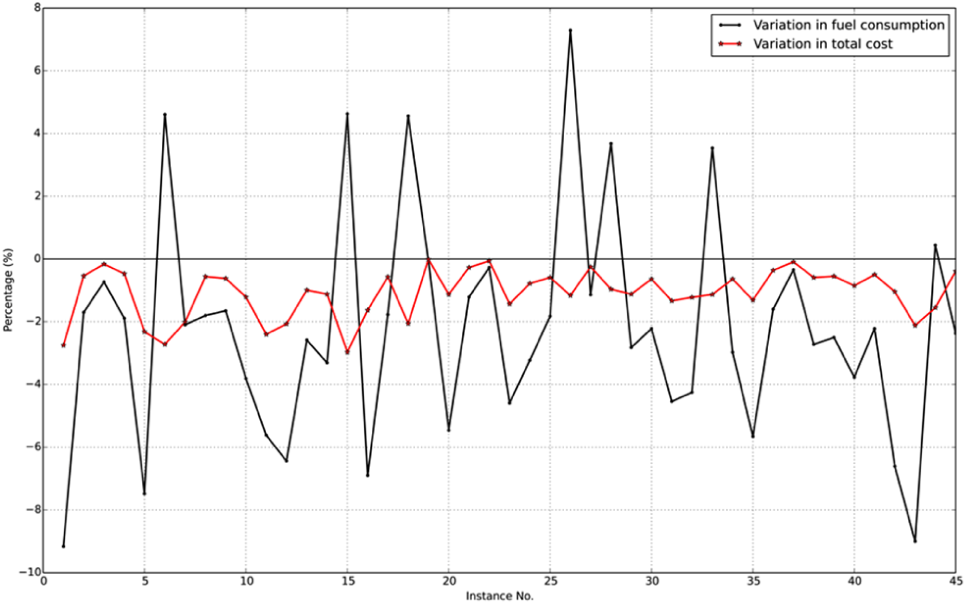
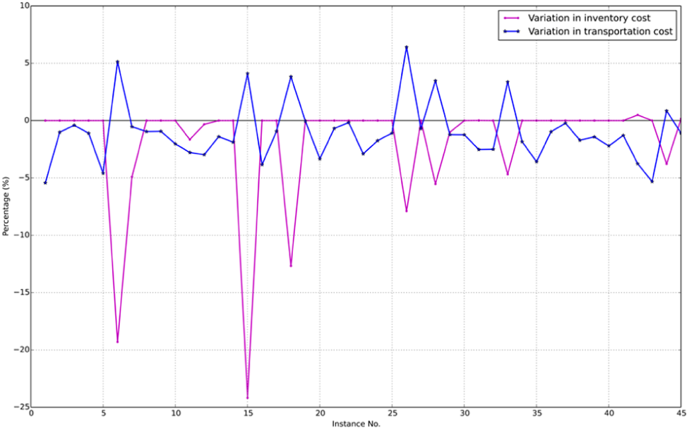
To study the differences between models, four aspects are compared: fuel consumption, inventory cost, transportation cost, and total cost. Only instances with optimal solutions under the time limit are reported. Note that in traditional MIRP, the amount of fuel consumption might be different for a given route, because the distance matrix is symmetric and a vehicle may travel from two opposite directions. In the following analyses, the worst-case fuel consumption is reported for the traditional model to indicate the maximal economic and environmental benefits which can be achieved from FCMIRP. Detailed comparison results are given in Table 1 and graphical comparison is presented in Figures 1 and 2. For ease of exposition, each instance is given a new number, for which refer to Table 1.

Table 1.

Detailed Comparison between the FCMIRP and the Traditional MIRP

No.	Instance	FCMIRP				Traditional MIRP				Gap (%)
No.	Instance	Fuel (L)	Inventory cost ($)	Transport cost ($)	Total cost ($)	Fuel (L)	Inventory cost ($)	Transport cost ($)	Total cost ($)	Fuel	Inventory cost	Transport cost	Total cost
1	10-1-1-3-1	142.94	225.88	231.66	457.54	156.03	225.88	244.23	470.11	−9.16	0.00	−5.43	−2.75
2	10-1-1-3-2	146.91	208.85	238.71	447.56	149.41	208.85	241.11	449.96	−1.70	0.00	−1.01	−0.54
3	10-1-1-3-3	92.64	239.77	162.80	402.57	93.31	239.77	163.45	403.22	−0.73	0.00	−0.40	−0.16
4	10-1-1-3-4	127.75	281.30	211.13	492.43	130.17	281.30	213.45	494.75	−1.89	0.00	−1.10	−0.47
5	10-1-1-3-5	179.55	273.79	281.04	554.83	192.98	273.79	293.93	567.72	−7.48	0.00	−4.59	−2.32
6	10-1-3-3-1	228.82	180.61	382.04	562.64	218.27	215.47	362.46	577.93	4.61	−19.30	5.13	−2.72
7	10-1-3-3-2	199.64	174.04	340.3	514.34	203.82	182.56	342.12	524.68	−2.10	−4.90	−0.53	−2.01
8	10-1-3-3-3	178.05	220.08	311.3	531.38	181.26	220.08	314.25	534.33	−1.80	0.00	−0.95	−0.56
9	10-1-3-3-4	200.75	168.97	341.5	510.47	204.06	168.97	344.68	513.65	−1.65	0.00	−0.93	−0.62
10	10-1-3-3-5	159.30	193.41	286.57	479.99	165.36	193.41	292.39	485.80	−3.81	0.00	−2.03	−1.21
11	10-1-5-3-1	214.20	203.92	396.33	600.24	226.23	207.28	407.36	614.64	−5.62	−1.65	−2.78	−2.40
12	10-1-5-3-2	194.80	190.79	370.98	561.77	207.34	191.41	381.99	573.40	−6.44	−0.32	−2.97	−2.07
13	10-1-5-3-3	253.05	189.79	446.57	636.35	259.58	189.79	452.84	642.63	−2.58	0.00	−1.40	−0.99
14	10-1-5-3-4	207.69	236.50	350.62	587.12	214.56	236.50	357.22	593.72	−3.31	0.00	−1.88	−1.12
15	10-1-5-3-5	290.00	165.49	495.75	661.24	276.56	205.51	475.35	680.86	4.63	−24.18	4.11	−2.97
16	10-1-1-5-3	206.90	479.58	353.74	833.32	221.17	479.58	367.31	846.89	−6.90	0.00	−3.84	−1.63
17	10-1-3-5-2	350.40	380.92	611.56	992.48	356.59	380.92	617.25	998.17	−1.77	0.00	−0.93	−0.57
18	10-1-3-5-5	351.23	360.42	647.94	1008.35	335.20	406.07	623.1	1029.17	4.56	−12.67	3.83	−2.06
19	20-1-1-3-1	194.32	522.88	301.82	824.71	194.44	522.88	301.93	824.81	−0.06	0.00	−0.04	−0.01
20	20-1-1-3-2	179.67	552.59	282.32	834.91	189.48	552.59	291.74	844.33	−5.46	0.00	−3.34	−1.13
21	20-1-1-3-3	160.55	386.60	254.4	641.00	162.49	386.60	256.13	642.73	−1.21	0.00	−0.68	−0.27
22	20-1-1-3-4	171.38	447.59	270.09	717.68	171.83	447.59	270.53	718.12	−0.27	0.00	−0.16	−0.06
23	20-1-1-3-5	230.76	360.69	351.16	711.86	241.35	360.69	361.33	722.02	−4.59	0.00	−2.90	−1.43
24	20-1-3-3-1	206.56	440.33	350.96	791.29	213.24	440.33	357.11	797.44	−3.23	0.00	−1.75	−0.78
25	20-1-3-3-2	271.27	361.31	438.05	799.37	276.20	361.31	442.78	804.09	−1.82	0.00	−1.08	−0.59
26	20-1-3-3-3	225.03	418.64	372.96	791.60	208.63	451.69	349.06	800.75	7.29	−7.89	6.41	−1.16
27	20-1-3-3-4	173.44	481.09	268.32	749.41	175.41	481.09	270.21	751.30	−1.14	0.00	−0.70	−0.25
28	20-1-3-3-5	221.94	360.41	370.38	730.79	213.76	380.35	357.48	737.83	3.68	−5.53	3.48	−0.96
29	20-1-5-3-1	276.93	411.56	478.67	890.23	284.75	415.70	484.5	900.20	−2.82	−1.01	−1.22	−1.12
30	20-1-5-3-2	277.29	448.62	479.67	928.28	283.45	448.62	485.58	934.20	−2.22	0.00	−1.23	−0.64
31	20-1-5-3-3	275.73	423.72	477.52	901.25	288.26	423.66	489.55	913.21	−4.54	0.01	−2.52	−1.33
32	20-1-5-3-4	248.58	428.00	406.31	834.31	259.15	428.00	416.45	844.45	−4.25	0.00	−2.50	−1.22
33	20-1-1-5-2	344.39	684.85	537.48	1222.33	332.19	716.87	519.3	1236.17	3.54	−4.68	3.38	−1.13
34	30-1-1-3-1	206.07	598.85	319.31	918.16	212.20	598.85	325.19	924.04	−2.97	0.00	−1.84	−0.64
35	30-1-1-3-2	240.21	633.86	363.34	997.20	253.80	633.86	376.39	1010.25	−5.66	0.00	−3.59	−1.31
36	30-1-1-3-3	224.93	571.96	342.46	914.42	228.52	571.96	345.78	917.74	−1.60	0.00	−0.97	−0.36
37	30-1-1-3-4	247.80	587.98	375.16	963.14	248.66	587.98	375.98	963.96	−0.34	0.00	−0.22	−0.09
38	30-1-1-3-5	218.64	626.66	333.31	959.98	224.57	626.66	339.01	965.67	−2.72	0.00	−1.71	−0.59
39	30-1-3-3-1	218.19	587.88	367.94	955.83	223.64	587.88	373.17	961.05	−2.50	0.00	−1.42	−0.55
40	30-1-3-3-2	247.86	651.09	404.84	1055.93	257.20	651.09	413.8	1064.89	−3.77	0.00	−2.21	−0.85
41	30-1-3-3-3	238.06	616.95	392.85	1009.8	243.35	616.95	397.93	1014.88	−2.22	0.00	−1.29	−0.50
42	30-1-3-3-4	222.05	658.25	371.91	1030.17	236.74	654.99	385.88	1040.87	−6.61	0.50	−3.76	−1.04
43	30-1-3-3-5	264.42	649.00	429.53	1078.53	288.22	649.00	452.38	1101.38	−9.00	0.00	−5.32	−2.12
44	30-1-5-3-1	323.47	580.91	540.69	1121.59	322.03	602.86	536.07	1138.93	0.44	−3.78	0.85	−1.55
45	30-1-5-3-2	271.55	562.45	436.51	998.96	277.99	561.55	441.27	1002.82	−2.37	0.16	−1.09	−0.39
	Average	224.57	409.53	372.86	782.39	228.97	414.86	375.80	790.66	−2.21	−1.89	−1.00	−1.09

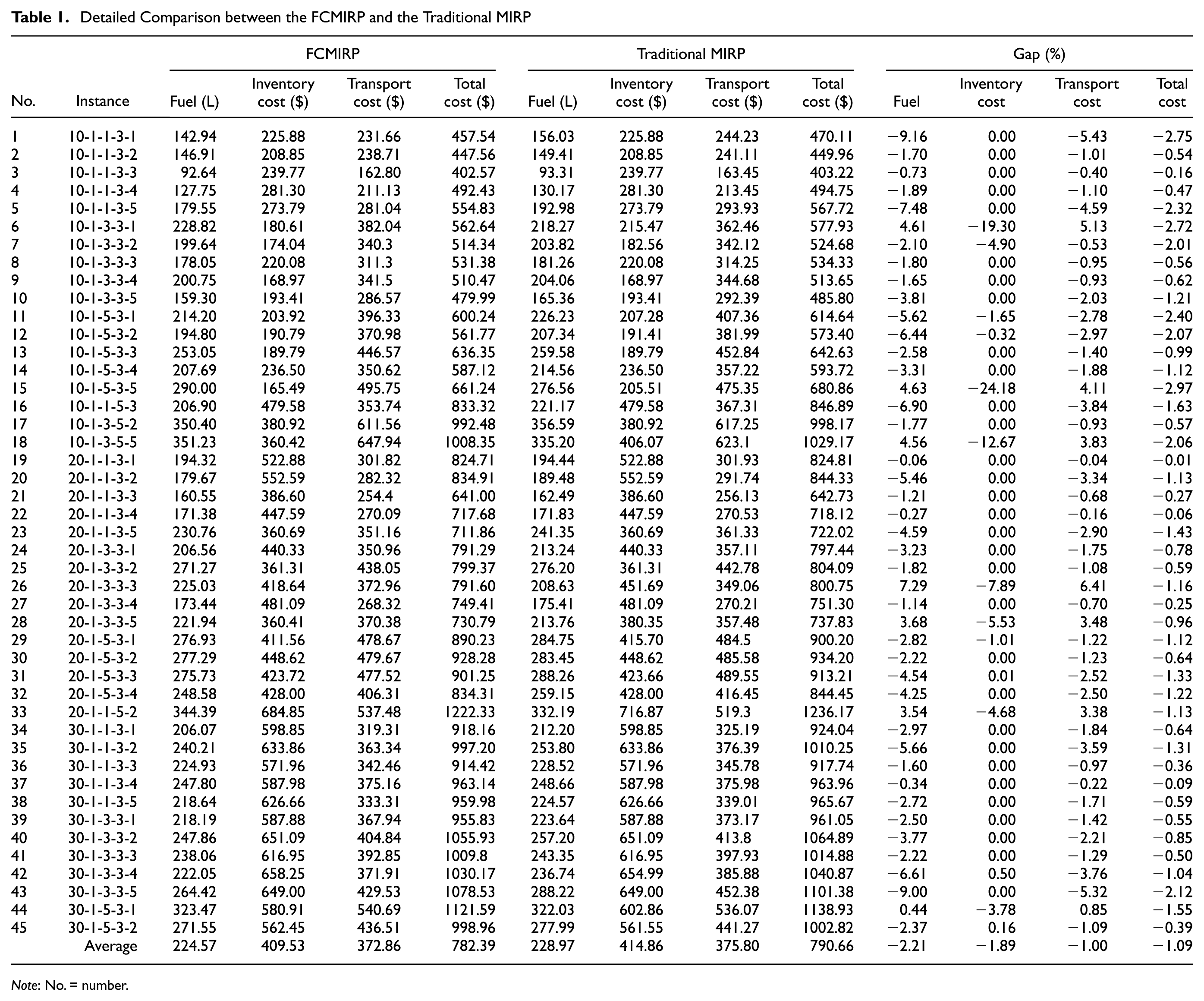
Note: No. = number.

Figure 1.

Gap in fuel consumption and total cost compared with traditional MIRP.

Figure 2.

Gap in inventory and transportation cost compared with traditional MIRP.

From Table 1 and Figure 1, in most instances (38 out of 45, about 84.4%), the fuel consumption of the FCMIRP is less, and it can achieve a saving of 2.21% on average. For instances 1, 5, 12, 16, 42, and 43, the saving is over 6%. Because fuel consumption is the direct cause of CO₂ emissions, the conclusion is that in most cases, FCMIRP can help enterprises achieve a better environmental benefit. Moreover, in all instances, FCMIRP generates solutions with lower cost, leading to an average saving of 1.09%. Figure 2 shows that in some cases, even though the inventory cost of the two models is the same, the transportation cost of the FCMIRP is lower, because less fuel is consumed. For instances 6, 15, 18, 26, 28, and 33, the transportation cost has a slight increase, to lower inventory cost. This suggests that considering fuel consumption in MIRP will lead to a new balance between inventory and transportation costs.

In seven instances, vehicles consume more fuel in the FCMIRP. This counter-intuitive phenomenon can be explained by the FCMIRP’s cost-oriented nature; sometimes a small increase in fuel consumption can lead to a large decrease in inventory cost, resulting in a lower total cost. In the following sections, four instances will be used to exemplify the specific differences in the solutions of these two models.

Route Direction and Order

FCMIRP will lead to a difference in route direction, because decision makers will only choose the direction in which vehicles consume less energy. However, in traditional MIRP, a vehicle may travel in either direction. Taking instance “10-1-1-3-1” as an example, in the two models the route length and inventory cost are the same whereas the route direction is converse, as shown in Table 2.

Table 2.

Instance 10-1-1-3-1 to Show the Difference in Route Direction

FCMIRP	Traditional MIRP
Period 1: No routePeriod 2: 0→9→4→5→6→2→3→1→10→0 (fuel consumption: 142.94)Period 3: No route	Period 1: No routePeriod 2: 0→10→1→3→2→6→5→4→9→0 (fuel consumption: 156.03)Period 3: No route

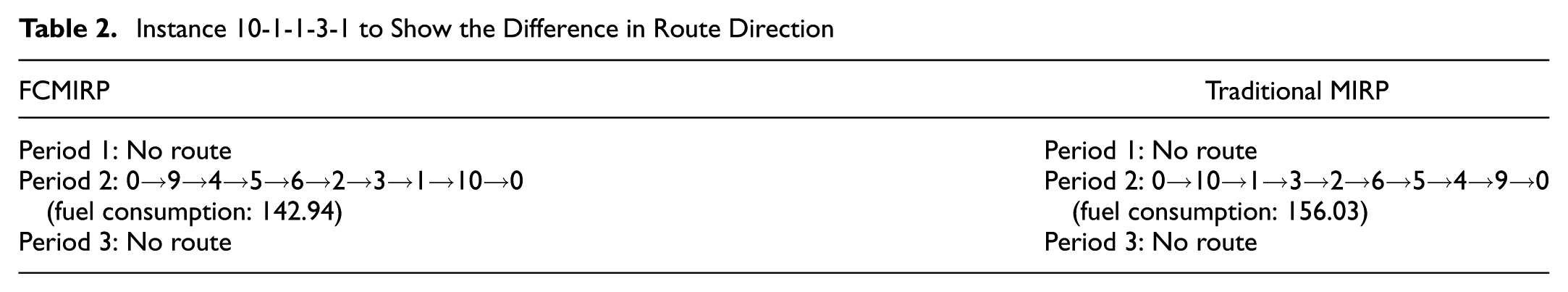
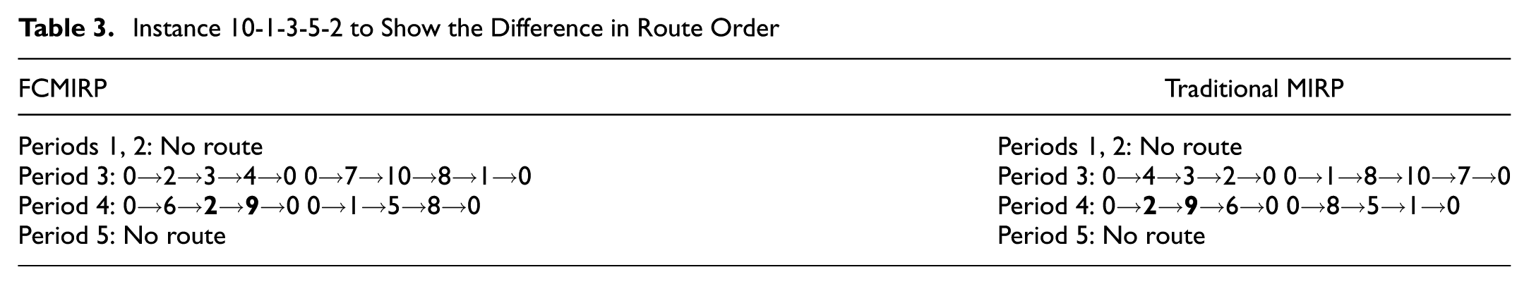
From Table 2 one may conclude that it is possible to directly transform traditional MIRP to FCMIRP by simply reversing the route direction, but this method does not always work. Take instance “10-1-3-5-2,” presented in Table 3, for example. For traditional MIRP, if one route in period 2 is reversed, becoming “0→6→9→2→0,” then the fuel consumption will be 47.64. However, if the visiting order of retailers 2 and 9 is further exchanged, just as the route in the FCMIRP, the fuel consumption will be 45.27. Therefore, a simple reverse operation cannot guarantee a maximal saving of energy.

Table 3.

Instance 10-1-3-5-2 to Show the Difference in Route Order

FCMIRP	Traditional MIRP
Periods 1, 2: No routePeriod 3: 0→2→3→4→0 0→7→10→8→1→0Period 4: 0→6→2→9→0 0→1→5→8→0Period 5: No route	Periods 1, 2: No routePeriod 3: 0→4→3→2→0 0→1→8→10→7→0Period 4: 0→2→9→6→0 0→8→5→1→0Period 5: No route

Inventory Strategy

Sometimes even though the routes of the two models are similar, their inventory strategy may be different. Take instance “10-1-5-3-1,” for example.

Table 4 shows that the routes of the two models are very similar except that retailer 7 is visited in different periods. For traditional MIRP, visiting retailer 7 in period 2 will reduce route length, result in lower driver cost and variable transportation cost. However, for FCMIRP, it is better to visit retailer 7 later, because its inventory holding cost coefficient is much higher than that of the supplier, and the saving of inventory cost will exceed the increase of driver cost.

Table 4.

Instance 10-1-5-3-1 to Show the Difference in Inventory Strategy

FCMIRP	Traditional MIRP
Periods 1: No routePeriod 2: 0→10(45)^a→4(116)→9(37)→5(28)→1(1)→00→2(61)→8(119)→0Period 3: 0→2(75)→7(24)→0	Period 1: No routePeriod 2: 0→10(45)→4(116)→9(37)→5(28)→1(1)→00→2(61)→8(119)→7(24)→0Period 3: 0→2(75)→0

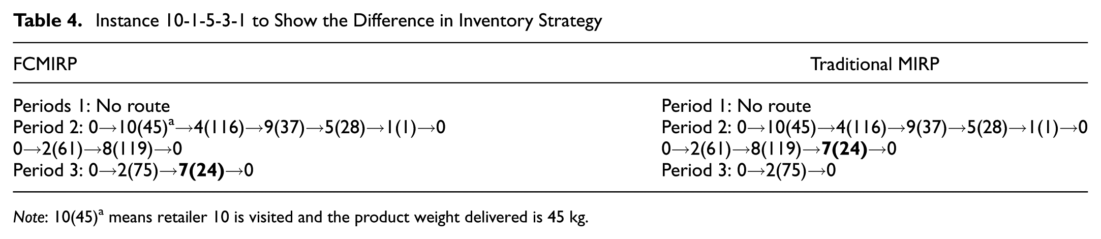
Note: 10(45)^a means retailer 10 is visited and the product weight delivered is 45 kg.

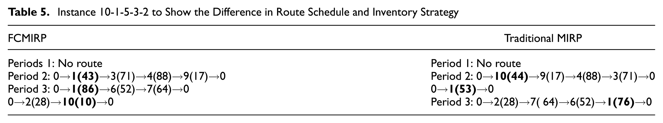
Route Schedule and Inventory Strategy

FCMIRP may result in a totally different route schedule and inventory strategy. Take instance “10-1-5-3-2” as an example, shown in Table 5. It demonstrates that the number of trips in each period is different and that the total product weight delivered to a retailer (such as retailer 10) varies. From instance data, the inventory holding cost coefficient of retailer 10 is 0; in traditional MIRP, then, more products are carried to the retailer, to control inventory cost, which on the other hand causes more fuel consumption.

Table 5.

Instance 10-1-5-3-2 to Show the Difference in Route Schedule and Inventory Strategy

FCMIRP	Traditional MIRP
Periods 1: No routePeriod 2: 0→1(43)→3(71)→4(88)→9(17)→0Period 3: 0→1(86)→6(52)→7(64)→00→2(28)→10(10)→0	Period 1: No routePeriod 2: 0→10(44)→9(17)→4(88)→3(71)→00→1(53)→0Period 3: 0→2(28)→7( 64)→6(52)→1(76)→0

To conclude, the solutions of the two models differ from each other in route direction, route order, and inventory strategy, which leads to a new tradeoff between inventory and transportation cost, and also generates different environmental implications.

Parameter Analyses

The study now examines the factors that may influence the decision of FCMIRP. The analyses are performed based on two randomly selected small instances (10-1-5-3-2, 10-1-5-3-3) and two medium instances (20-1-3-3-3, 20-1-1-5-2), because they are more time-efficient compared with large ones.

Distance Factor

The distance between nodes in the previous test has been scaled down, to consider the situation that during each trip the driver’s work time is shorter than 8 h (actually the results show that the average work time is 5.12 h per trip). Here this constraint is relaxed to model the case of long distance transport, in order to figure out FCMIRP’s potential for this application. The process in this case is to gradually increase the distance between nodes by changing α from 6 to 2 and observe its effect (Figure 3); other parameters’ values are the same as already given above as instance data.

Figure 3.

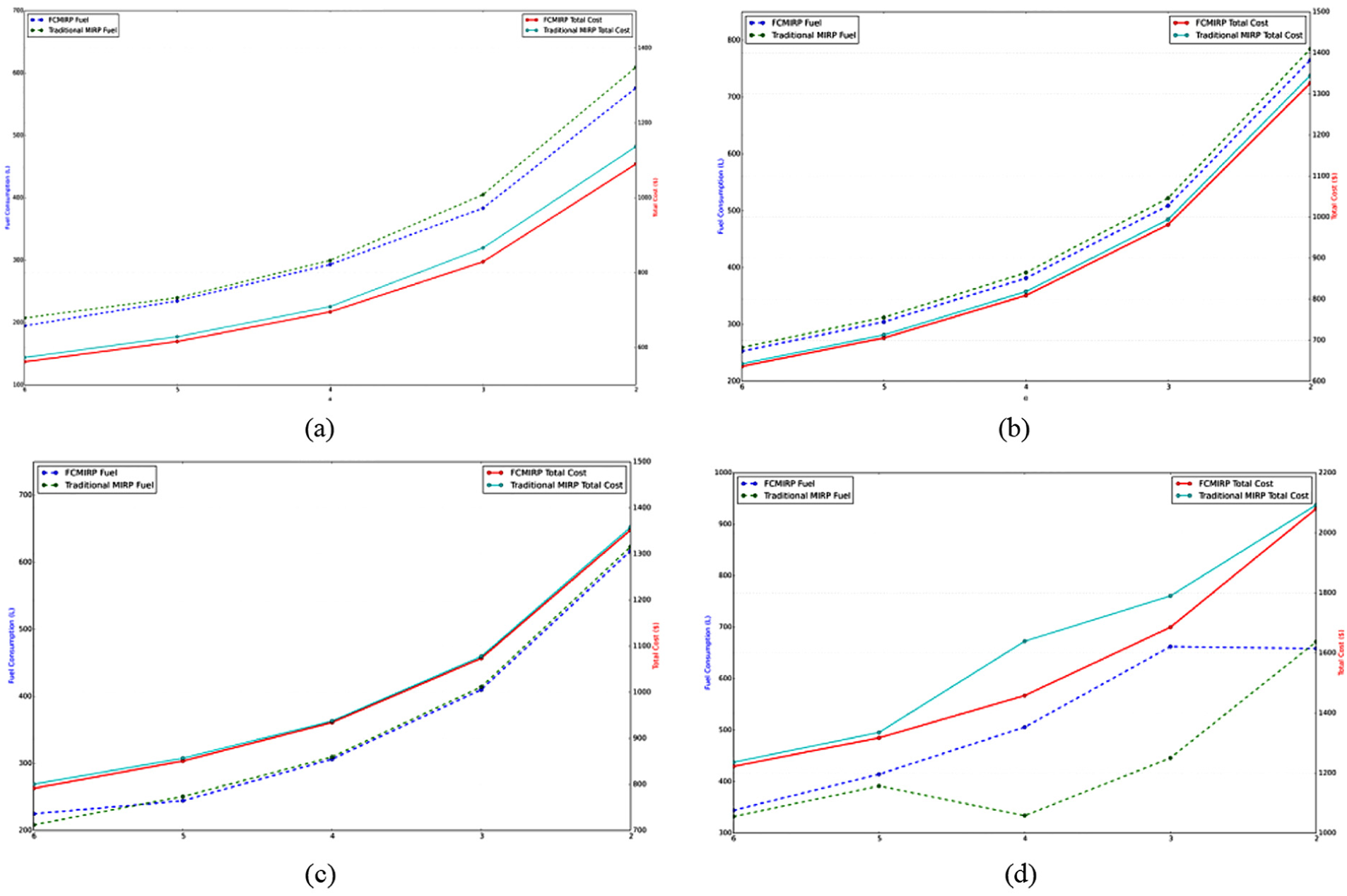
The influence of the distance factor for (a) instance 10-1-5-3-2, (b) instance 10-1-5-3-3, (c) instance 20-1-3-3-3, and (d) instance 20-1-1-5-2.

Figure 3 shows that as distance increases the total cost will increase as expected in these two models. However, the total cost of the FCMIRP is lower under any case. The average saving for each instance is 2.99%, 1.18%, 0.60%, and 4.34%, respectively. The maximal saving is 12.41% for instance 20-1-1-5-2 with α = 4. Thus, the conclusion is that the FCMIRP is also capable of saving cost for long distance transport, and sometimes it has a great potential to reduce cost.

The general fuel consumption trend is increasing for both models. For the first two instances, the FCMIRP can save 4.45% and 2.57% fuel on average. For the last instance, FCMIRP consumes more fuel in order to lower inventory cost and total cost.

Unit Fuel Price

For FCMIRP, u is changed step by step and its influence on fuel consumption and inventory cost is observed (Figure 4).

Figure 4.

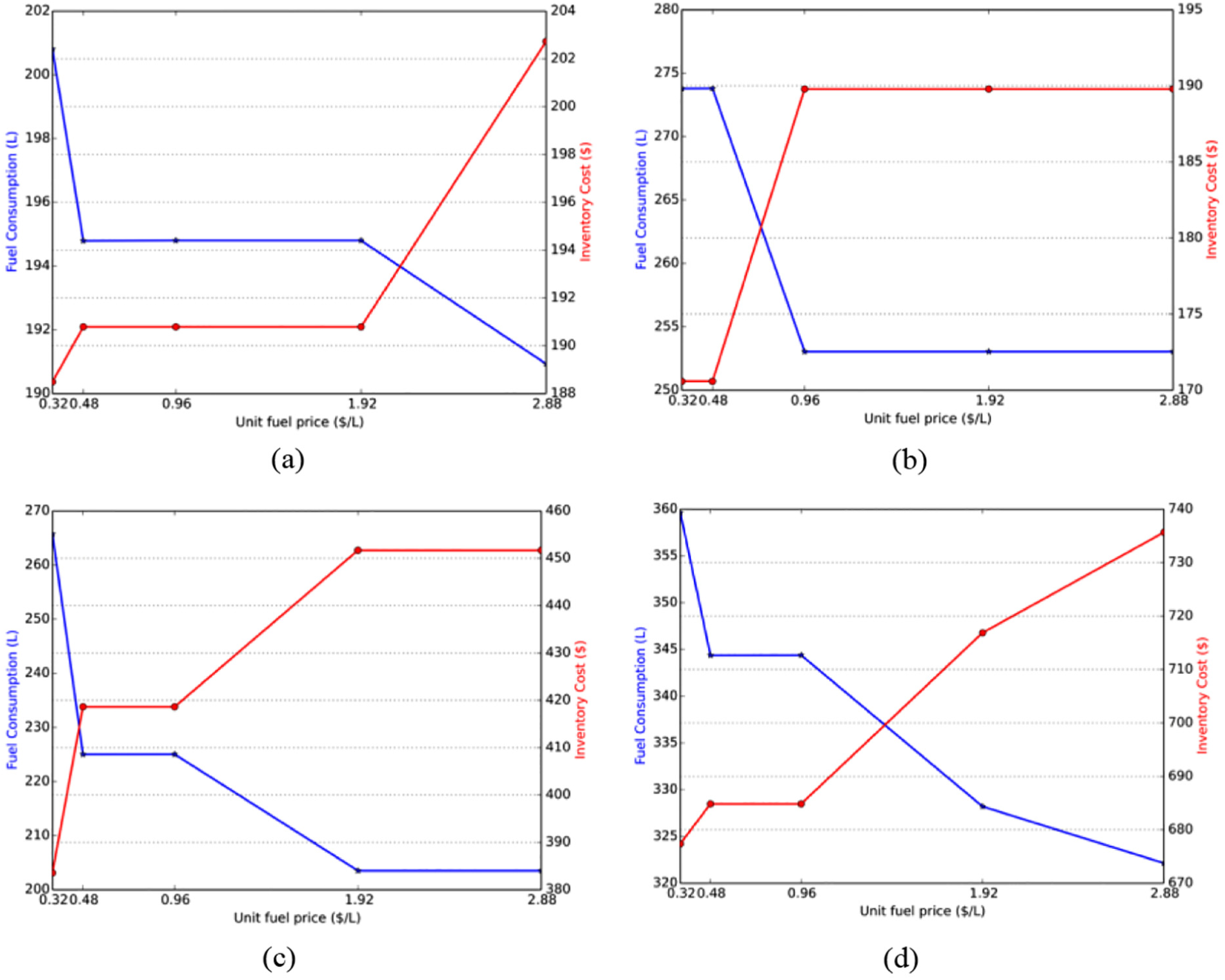
Trend of inventory cost and fuel consumption as u changes for (a) instance 10-1-5-3-2, (b) instance 10-1-5-3-3, (c) instance 20-1-3-3-3, and (d) instance 20-1-1-5-2.

As expected, when u increases the general trend of inventory cost is increasing and that of fuel consumption is decreasing. However, the process reveals that sometimes when the fuel price varies, both the inventory cost and fuel consumption remain constant. In these situations, if decision makers choose to further increase inventory expenses, it will cost more money, more than the decrease of transportation cost. Therefore, it is better to keep the current decisions. Because CO₂ emissions and fuel consumption are linearly dependent, it is also possible to recognize the fuel price here as an emission price (or carbon tax). Then Figure 4 can also represent the trend of CO₂ emissions with varying carbon taxing. Thus, the conclusion is that a higher fuel or emission price does not always mean a lower emission level.

Fleet Size

Instances 10-1-5-3-2 and 20-1-3-3-3 are used to analyze the influence of fleet size, as shown in Table 6. Constraint (23) is added to both models, where s is the maximal allowable trip number in each period. Meanwhile, the vehicle capacity is halved in each instance.

\sum_{j \in V'} x_{0 j}^{t} \leq s t \in T

(23)

Table 6.

The Influence of Fleet Size

	10-5-3-2						20-3-3-3
	FCMIRP		Traditional MIRP		Gap (%)			FCMIRP		Traditional MIRP		Gap (%)
s	Fuel	Cost	Fuel	Cost	Fuel	Cost	s	Fuel	Cost	Fuel	Cost	Fuel	Cost
2	282.13	770.68	291.51	780.43	−3.32	−1.27	1	270.55	928.63	283.33	942.81	−4.72	−1.53
3	282.13	767.32	291.51	777.07	−3.32	−1.27	2	270.32	897.66	281.19	908.53	−4.02	−1.21

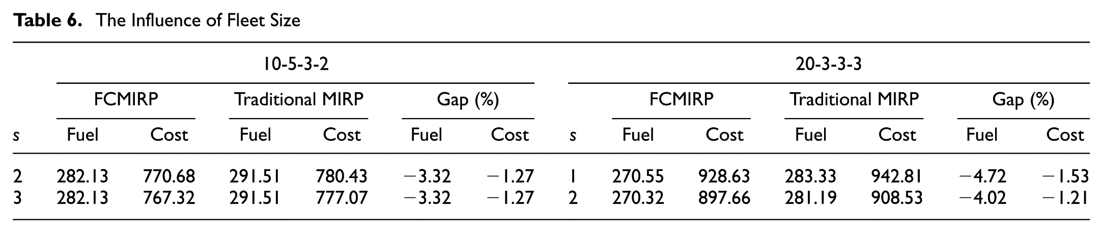
Table 6 shows that FCMIRP can still save fuel and total cost when this new constraint is added. As expected, when the allowable trip number is small, the total cost will increase, which mainly results from increasing inventory cost. This is because if fewer vehicles are available, it is necessary to move some trips to the next a few periods to be executed, and the inventory holding cost coefficient of the supplier is higher than that of some retailers.

Conclusion

This paper addresses a MIRP with environmental consideration. It is different from previous studies in that a new model considering fuel consumption is proposed, which can help enterprises make a more accurate tradeoff between transportation and inventory costs, and assist them to lower fuel consumption and CO₂ emissions. Numerical tests demonstrate that FCMIRP indeed generates different vehicle schedules and inventory strategies. For all instances, the FCMIRP is capable of saving overall cost, and in most cases it can decrease fuel consumption and CO₂ emissions.

Based on the numerical tests, it is possible to derive managerial insights from two points of view: (1) enterprises should reconsider their inventory replenishment (tactic) plan and vehicle routing (operational) plan by taking fuel consumption into account, as these have been proved to be quite different from the traditional distance-based plans; and (2) for government regulators, higher fuel prices or carbon taxing do not always lead to a better environmental benefit, because to pursue overall profits, enterprises may sacrifice transportation costs (therefore more emissions) for savings in inventory costs in cases in which inventory costs are a major component.

Future studies could be conducted on two aspects of the problem. First, it would be possible to develop powerful heuristic algorithms to solve large FCMIRP instances. Second, more factors, such as vehicle speed, road angles, and different vehicle types, could be incorporated when calculating fuel consumption.

Footnotes

Acknowledgements

This work is supported by the National Natural Science Foundation of China (71772100), Shenzhen Science and Technology Project (JCYJ20170412171044606), and National Key Technologies Research and Development Program (2016YFB0502601, 2016YFC0803107). The authors would like to thank anonymous referees for their helpful comments.

Author Contributions

The authors confirm contribution to the paper as follows: study conception and design: Cheng, C., Qi, M.; data collection: Cheng, C.; analysis and interpretation of results: Cheng, C., Qi, M., Rousseau, L. M; draft manuscript preparation: Cheng, C, Rousseau, L. M. All authors reviewed the results and approved the final version of the manuscript.

The Standing Committee on Freight Transportation Planning and Logistics (AT015) peer-reviewed this paper (18-00143).

References

Lin

Choy

K. L.

G. T. S.

Chung

S. H.

Lam

H. Y.

Survey of Green Vehicle Routing Problem: Past and Future Trends. Expert Systems with Applications, Vol. 41, No. 4 PART 1, 2014, pp. 1118–1138. https://doi.org/10.1016/j.eswa.2013.07.107.

Kara

B. Y.

Yetis

M. K.

Energy Minimizing Vehicle Routing Problem. In Combinatorial Optimization and Applications: First International Conference, COCOA 2007, Xi’an, China, August 14-16, 2007. Proceedings ( Dress

Zhu

, eds.), Springer Berlin Heidelberg, Berlin, Heidelberg, pp. 62–71.

Salimifard

Shahbandarzadeh

Raeesi

Green Transportation and the Role of Operation Research. Proc., 2012 International Conference on Traffic and Transportation Engineering, Vol. 26, Singapore, IACSIT Press 2012, pp. 74–79.

Xiao

Zhao

Kaku

Development of a Fuel Consumption Optimization Model for the Capacitated Vehicle Routing Problem. Computers and Operations Research, Vol. 39, No. 7, 2012, pp. 1419–1431. https://doi.org/10.1016/j.cor.2011.08.013.

Zhang

Lee

C. K. M.

Choy

K. L.

W. H.

Design and Development of a Hybrid Artificial Bee Colony Algorithm for the Environmental Vehicle Routing Problem. Transportation Research Part D: Transport and Environment, Vol. 31, 2014, pp. 85–99. https://doi.org/10.1016/j.trd.2014.05.015.

Bell

W. J.

Dalberto

L. M.

Fisher

M. L.

Greenfield

A. J.

Jaikumar

Kedia

Mack

R. G.

Prutzman

P. J.

Improving the Distribution of Industrial Gases with an On-Line Computerized Routing and Scheduling Optimizer. Interfaces, Vol. 13, No. 6, 1983, pp. 4–23.

Andersson

Hoff

Christiansen

Hasle

Løkketangen

Industrial Aspects and Literature Survey: Combined Inventory Management and Routing. Computers and Operations Research, Vol. 37, No. 9, 2010, pp. 1515–1536. https://doi.org/10.1016/j.cor.2009.11.009.

Coelho

L. C.

Cordeau

J. F.

Laporte

Thirty Years of Inventory Routing. Transportation Science, Vol. 48, No. 1, 2014, pp. 1–19. https://doi.org/10.1287/trsc.2013.0472.

Huang

S. H.

Lin

P. C.

A Modified Ant Colony Optimization Algorithm for Multi-Item Inventory Routing Problems with Demand Uncertainty. Transportation Research Part E: Logistics and Transportation Review, Vol. 46, No. 5, 2010, pp. 598–611. https://doi.org/10.1016/j.tre.2010.01.006.

10.

Moin

N. H.

Salhi

Aziz

N. A. B.

An Efficient Hybrid Genetic Algorithm for the Multi-Product Multi-Period Inventory Routing Problem. Vol. 7595, No. 225, 2011, pp. 1–21. https://doi.org/10.1016/j.ijpe.2010.06.012.

11.

Coelho

L. C.

Laporte

A Branch-and-Cut Algorithm for the Multi-Product Multi-Vehicle Inventory-Routing Problem. International Journal of Production Research, Vol. 51, No. 23–24, 2013, pp. 7156–7169. https://doi.org/10.1080/00207543.2012.757668.

12.

Archetti

Bertazzi

Laporte

Speranza

M. G.

A Branch-and-Cut Algorithm for a Vendor-Managed Inventory-Routing Problem. Transportation Science, Vol. 41, No. 3, 2007, pp. 382–391. https://doi.org/10.1287/trsc.1060.0188.

13.

Coelho

L. C.

Laporte

The Exact Solution of Several Classes of Inventory-Routing Problems. Computers and Operations Research, Vol. 40, No. 2, 2013, pp. 558–565. https://doi.org/10.1016/j.cor.2012.08.012.

14.

Desaulniers

Rakke

J. G.

Coelho

L. C.

A Branch-Price-and-Cut Algorithm for the Inventory-Routing Problem. Transportation Science, Vol. 50, No. 3, 2015, pp. 1060–1076. https://doi.org/10.1287/trsc.2015.0635

15.

Mjirda

Jarboui

Macedo

Hanafi

Mladenović

A Two Phase Variable Neighborhood Search for the Multi-Product Inventory Routing Problem. Computers and Operation Research, Vol. 52, 2014, pp. 291–299. https://doi.org/10.1016/j.cor.2013.06.006.

16.

Zachariadis

E. E.

Tarantilis

C. D.

Kiranoudis

C. T.

An Integrated Local Search Method for Inventory and Routing Decisions. Expert Systems with Applications, Vol. 36, No. 7, 2009, pp. 10239–10248. https://doi.org/10.1016/j.eswa.2009.01.069.

17.

Seuring

A Review of Modeling Approaches for Sustainable Supply Chain Management. Decision Support Systems, Vol. 54, No. 4, 2013, pp. 1513–1520. https://doi.org/10.1016/j.dss.2012.05.053.

18.

Brandenburg

Govindan

Sarkis

Seuring

Quantitative Models for Sustainable Supply Chain Management: Developments and Directions. European Journal of Operational Research, Vol. 233, No. 2, 2014, pp. 299–312.

19.

Cinar

Gakis

Pardalos

P. M.

A 2-Phase Constructive Algorithm for Cumulative Vehicle Routing Problems with Limited Duration. Expert Systems with Applications, Vol. 56, 2016, pp. 48–58.

20.

Bektaş

Laporte

The Pollution-Routing Problem. Transportation Research Part B: Methodological, Vol. 45, No. 8, 2014, pp. 1232–1250. https://doi.org/10.1016/j.trb.2011.02.004.

21.

Koç

Ç.

Koç

Ç.

Bekta

Jabali

Laporte

The Fleet Size and Mix Pollution-Routing Problem. Transportation Research Part B: Methodological, Vol. 70, 2014, pp. 239–254. https://doi.org/10.1016/j.trb.2014.09.008.

22.

Martínez

J. C. V.

Fransoo

J. C.

Green Facility Location. In Sustainable Supply Chains ( Bouchery

Corbett

C. J.

Fransoo

J. C.

Tan

, eds.), Springer International Publishing, New York, 2017, pp. 219–234.

23.

Dekker

Bloemhof

Mallidis

Operations Research for Green Logistics: An Overview of Aspects, Issues, Contributions and Challenges. European Journal of Operational Research, Vol. 219, No. 3, 2012, pp. 671–679. https://doi.org/10.1016/j.ejor.2011.11.010.

24.

Treitl

Nolz

P. C.

Jammernegg

Incorporating Environmental Aspects in an Inventory Routing Problem: A Case Study from the Petrochemical Industry. Flexible Services and Manufacturing Journal, Vol. 26, No. 1–2, 2014, pp. 143–169. https://doi.org/10.1007/s10696-012-9158-z.

25.

Soysal

Bloemhof-Ruwaard

J. M.

Haijema

van der Vorst

J. G. A. J.

Modeling a Green Inventory Routing Problem for Perishable Products with Horizontal Collaboration. Computers and Operations Research, Vol. 89, 2018, pp.168–182. https://doi.org/10.1016/j.cor.2016.02.003.

26.

Coelho

L. C.

Laporte

Improved Solutions for Inventory-Routing Problems through Valid Inequalities and Input Ordering. International Journal of Production Economics, Vol. 155, 2014, pp. 391–397. https://doi.org/10.1016/j.ijpe.2013.11.019.

27.

Ubeda

Arcelus

F. J.

Faulin

Green Logistics at Eroski: A Case Study. International Journal of Production Economics, Vol. 131, No. 1, 2011, pp. 44–51. https://doi.org/10.1016/j.ijpe.2010.04.041.