
Abstract
State agencies, regional agencies, cities, towns, and local municipalities design and maintain transportation systems for the benefit of users by improving mobility, reducing travel time, and enhancing safety. Cost–benefit analysis based on travel time savings and the value of reliability helps these agencies in prioritizing transportation projects or when evaluating transportation alternatives. This paper illustrates the use of monetary values of travel time savings and travel time reliability, computed for the state of North Carolina, to help assess the impact of transportation projects or alternatives. The results obtained indicate that, based on the illustration of the effect and impact of various transportation projects or alternatives, both improved travel time and reliability on roads yield significant monetary benefits. However, from cost–benefit analysis, it is observed that greater benefits can be achieved through improved reliability compared with benefits from a decrease in travel time for a given section of road.
Travel demand has progressively increased with the development of modern civilization and the need for more travel over the past few decades. The subsequent effect of this increasing travel demand is recurring congestion on a limited road network, a growing air quality problem, and the lack of safe and reliable transportation systems. New roads are being constructed, existing roads are being widened, or alternate modes of transportation are being explored to reduce congestion and handle the growth. However, resource constraints (funding limitations) fueled by effective utilization of resources compel practitioners to assess the impact of transportation projects or alternatives before prioritization and implementation.
For years, it has been assumed that the fastest path from an origin to a destination is used by most motorists. These motorists usually plan for some expected delay caused by recurring congestion, which is common today in many urban areas. Further, motorists’ approach toward trip planning seems to be changing because of fluctuations and uncertainty in traffic conditions. The unexpected or nonrecurring congestion caused by crashes, inclement weather, construction activity, and special events contributes most to these fluctuations and the uncertainty ( 1 – 4 ). Therefore, reliability (consistency or dependability in travel time) of a route is playing a more prominent role in departure and route choice decisions among various other travel time performance measures.
Reliability is defined as the probability that a component or system will perform a required function (without failure) for a given period of time, when used under stated operating conditions ( 5 ). For assessing travel time reliability or travel time variation, numerous indices were proposed by researchers in the past. The Federal Highway Administration recommends five standard measures of travel time reliability: 90th or 95th percentile travel time, travel time index (TTI), planning time index (PTI), buffer time index (BTI), and frequency that congestion exceeds some expected threshold ( 6 ). Lomax et al. grouped reliability related performance measures into three categories: statistical range, buffer time (BT) measures, and tardy trip indicators ( 7 ). The value of these performance measures and how they could be used to assess transportation projects or alternatives is vital as they are expected to be widely used in transportation planning, for project prioritization, and for allocation of resources.
The value of time refers to the monetary value travelers place on reducing their travel time. There exists a vast body of literature on the theoretical underpinning of the value of travel time ( 8 – 11 ), on travel time savings ( 12 , 13 ), and to a lesser extent on the value of reliability ( 14 – 20 ). Most of the past studies document limited and inconclusive research on the value of reliability, particularly based on motorists’ perceptions.
Cost–benefit analysis helps state agencies, regional agencies, cities, towns, and local municipalities in prioritizing transportation projects/alternatives. It helps them efficiently and effectively use the limited available resources. In the cost–benefit analysis, the effect and impact of various transportation projects or alternatives are monetized to assess and make improved decisions. Currently, there exists limited documentation on the illustration and applicability of evaluating reliability, the value of travel time savings, and the value of reliability to assist with such decisions. Therefore, the objective of this paper is to illustrate the use and applicability of the value of travel time savings and the value of reliability to evaluate transportation projects or alternatives.
Monetary Values of Travel Time and Reliability
Pulugurtha et al. recently conducted a preliminary random general survey, followed by focus group survey and final random survey, to collect data and evaluate motorists’ perceptions of reliability ( 20 ). The preliminary random general survey consisted of questions which were aimed at capturing stated preference choices to evaluate how the participants would react to hypothetical situations. Based on the results from preliminary random general survey of 417 participants, the average travel time for daily commute in the state of North Carolina is 23.47 min. The average additional trip time (planned maximum BT) is equal to 10.54 min. It does not seem to vary based on the average travel time. Some differences were observed in evaluation based on the income level of the participant. Low income group participants followed by high income group participants tend to plan for higher additional trip time than medium income participants. Males tend to choose an unreliable route more often than females. This indicates a difference in perception toward additional trip time by gender.
The generalized value of travel time for North Carolina is estimated to be $ 0.51 per minute. The generalized value of additional trip time is also $ 0.51, and participants are willing to pay, on average, $ 0.11 to reduce travel time by 1 min ($6.46 per hour). The value of additional trip time was observed to be different for peak and off-peak hours. It was also observed to vary by gender and income group of the participant. The computed value of additional trip time can be used as the maximum value of BT to evaluate the benefits of a proposed/designed transportation project/alternative.
Nine focus group meetings were carried out across North Carolina to collect data from 93 participants as a part of the research. The participants of the focus group survey were asked to choose between a reliable route and an unreliable route. The focus group survey aimed to observe participants’ tradeoff between travel time savings and reliability. The results obtained from focus group survey indicate that higher percentages of participants are willing to opt for routes with a lower number of days of unreliability, as they will have some travel time savings. However, as the unreliability increases (number of days), participants start shifting from an unreliable route to a reliable route. The generalized value of BT for North Carolina based on focus group survey is estimated as $ 0.48 per minute. However, the focus group sample did not seem to be a good representation of the North Carolina population. Therefore, this was followed by the final random survey.
The final random survey comprised 357 participants who were asked to choose between two routes, a reliable route with longer travel time and an unreliable route with shorter travel time (as in the case of focus group survey). The maximum tolerance limit for unreliability is observed to be 4 days a month for a maximum BT of 20 min for a typical work day trip (∼23 min).
Differences were observed when the findings from the final random survey were compared with the focus group survey. The generalized value of BT for North Carolina based on the final random survey is estimated as $ 0.45 per minute. This is based on the maximum BT that participants are willing to accept by selecting an unreliable route, hoping to save travel time for most of the trips, before choosing a reliable route. This value is less than the value of additional trip time from the preliminary random general survey and the value of BT from the focus group survey. It is recommended for use to evaluate the impact of transportation projects or alternatives, in addition to the generalized value of travel time. The monetary values of travel times and reliability estimated as a part of the research conducted for the North Carolina Department of Transportation (NCDOT) were used for illustration purposes in this paper.
Readers are encouraged to refer to Pulugurtha et al. for more details related to surveys conducted, sample, perceptions of participants, the value of reliability, and thresholds ( 20 , 21 ).
Value of Travel Time Savings: Illustration
The estimated generalized value of travel time savings for the state of North Carolina is $6.46 per hour for every motorist. This value of travel time savings can be used to evaluate the benefits from a proposed/designed transportation project/alternative. First, the costs associated with the implementation of a transportation project/alternative are evaluated. Then, the benefits associated with the implementation of the transportation project/alternative (i.e., travel time savings in this case) are monetized. The costs and benefits are then compared to evaluate the breakeven period and overall returns. Along with the travel time savings, there could be other user benefits such as vehicle operating cost savings and some safety benefits, which are not considered in illustrating the costs and associated benefits, in the following examples.
Example: Estimating the Benefits of Proposed Improvements
Consider the design and construction of an additional lane on a 5-mi road to relieve congestion. Assume that the total cost of the proposed additional lane is $6,000,000 and that the project is to be completed by year 2020. The present value of the project can be computed using

where
PV = Present value,
FV = Future value,
i = discount rate (3%), and
n = difference between the year of analysis and the year of costs and benefits being evaluated.
Assume that the average travel time savings per person after adding the lane amount to 25 s. Similarly, the total vehicle miles of travel (VMT) on this 5-mi facility are 10,000 vehicle miles per hour during morning and evening peak hours (total 4 h). Because there could be multiple passengers in a vehicle, consider the average occupancy rate of 1.20 passengers per vehicle to evaluate total passenger miles of travel (PMT) during each peak hour. The total PMT during morning and evening peak hours (2 h in the morning and 2 h in the evening, total 4 h) is 10,000 * 1.2 * 4 = 48,000. Table 1 summarizes the total cost savings for the proposed design considering the analysis timeframe of 25 years. Many values considered in the table can be obtained from the regional travel demand forecasting model outputs.
Total Present Costs and Benefits for the Proposed Design
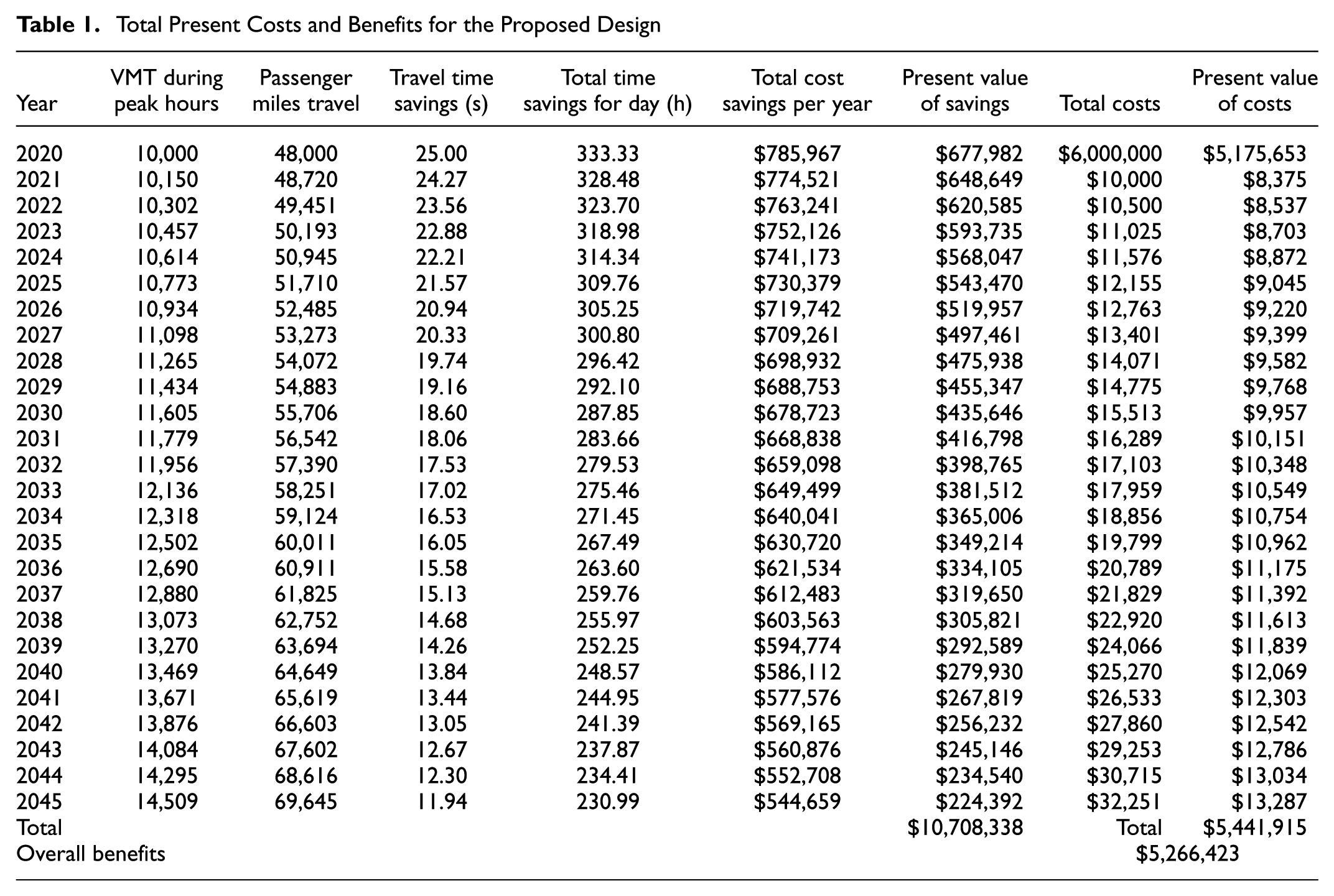
In the table, column 1 shows the time frame year, column 2 shows the VMT with an incremental rate of 1.5% each year, and column 3 shows the PMT for each year. With an increase in VMT, the travel time savings could decrease. Column 4 shows the travel time savings for each year with a 3% decrease in travel time savings, each year, from the previous year. Column 5 shows total travel time savings each day in hours and column 6 shows the total cost savings for each year. The cost savings are converted to 2015 dollars and are presented in column 7. Column 8 shows the cost incurred for implementation of the proposed design and other maintenance costs, each year, and column 9 shows the costs incurred in 2015 dollars. Overall, the proposed project will result in savings equal to $10,708,338 just because of reduced travel times. The savings could be even higher by considering reduced vehicle maintenance costs and improved safety. Considering a timeframe of 25 years, the overall benefit of the proposed design is $5,266,423.
Like the above example, a real-world scenario is considered to illustrate the benefits of proposed improvements. For this purpose, widening of a 10.3-mi section from four lanes to six lanes on I-40 South of Trinity Road, Raleigh is considered. The travel times decreased by 3.7 min and 5.5 min during morning peak hour and evening peak hour, after widening the road. With $6.46 per hour travel time saving value, the traffic volume after completion of road widening is considered to evaluate the cost savings from widening the road.
Table 2 shows the overall cost savings during peak hours on widening the I-40 section. The cost savings are estimated as $3,059 and $4,974 for morning peak hour and evening peak hour, respectively. Considering an overall of 4 h of peak volume on a given day (2 h in the morning and 2 h in the evening), the total cost savings in a year just during peak hours, because of widening the 10.3-mi section, are estimated as $5.86 million.
Cost Benefits from Widening of I-40
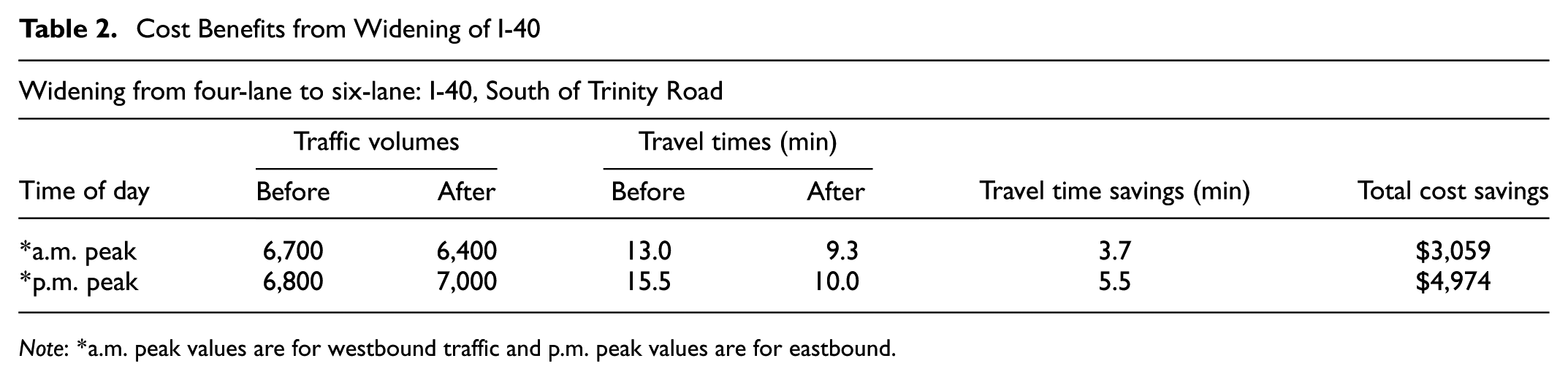
Note: *a.m. peak values are for westbound traffic and p.m. peak values are for eastbound.
Example: Evaluating Transportation Alternatives
For illustration, two hypothetical alternative designs (Alternative A and Alternative B) for a road alignment between two points are considered. The cost of Alternative A is $80 million and the cost of Alternative B is $100 million. After the construction of the alignment in year 2020, assume the average VMT per day on the proposed road is 120,000. Table 3 shows the comparison of benefits and costs between the two alternatives. Many values considered in the table (from column 2 to column 6) can be obtained from the regional travel demand forecasting model outputs.
Comparison of Costs and Benefits between Two Alternatives
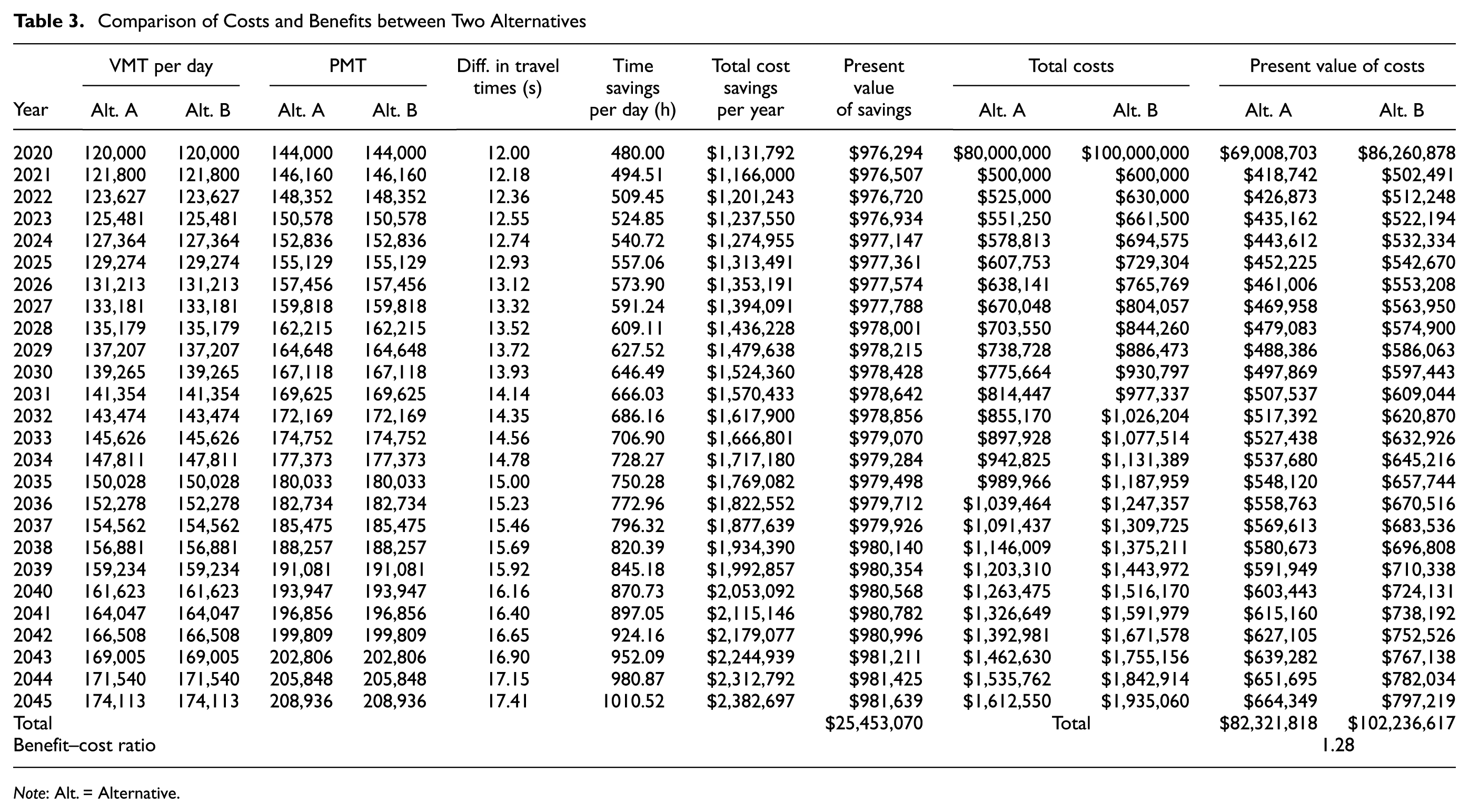
Note: Alt. = Alternative.
In Table 3, column 1 shows the year of analysis with a timeframe of 25 years; columns 2 and 3 show the VMT for both alternatives (which are the same) each year with a 1.5% increase in VMT each year; columns 4 and 5 show the PMT for both alternatives considering an average vehicle occupancy rate of 1.20; column 6 shows the travel time savings for Alternative B compared with Alternative A; column 7 shows the total time saving each day in hours; column 8 shows the total cost benefits each year from 2020 to 2045; column 9 shows the cost benefits as 2015 dollars; and, columns 10 to 13 show the overall costs including maintenance, each year, along with their respective 2015 costs.
The benefit–cost (B/C) ratio will help agencies evaluate transportation alternatives easily. The benefit–cost ratio is calculated as the ratio of total present value of the benefits between alternatives (sum of discounted benefits) to the discounted value of incremental costs (difference between the present values of cost of both the alternatives). If the B/C ratio is greater than 1, then the alternative considered is beneficial compared with the other alternative. From Table 3, the overall cost benefits from Alternative B over Alternative A are $25,453,070. The cost difference between the alternatives is $19,919,799 (Alternative B total cost – Alternative A total cost). The B/C ratio is 1.28, which is to say that Alternative B is more beneficial when compared with Alternative A, with a return on investments of $1.28 for every $1 spent. The procedure is repeated until all alternatives are considered to evaluate the most economically feasible alternative.
Reliability by Time-of-the-Day: Illustration
The reliability of a link or segment could vary based on the time-of-the-day. The possibility of capturing extensive, continuous, and dynamic travel time data from private sources such as HERE, INRIX and Tom Tom opened many pragmatic avenues to predict reliability at link-level by time-of-the-day ( 22 , 23 ). BT was observed to be strongly correlated to most travel time performance measures and may be suitable for assessing reliability ( 22 , 23 ). As sum of deviations is not the same as deviations of sums, data/measures should be carefully integrated when conducting path-level assessments (not used in the illustrations discussed in this paper).
Data from INRIX, for the year 2011, was used to illustrate the reliability of links by time-of-the-day and day-of-the-week (representative of general traffic conditions, with no construction activity within the vicinity of study segments). Travel time performance measures such as average travel time and 95th percentile travel time were computed by time-of-the-day and day-of-the-week for road links in the Charlotte metropolitan area. For illustration purposes, a 2.1-mi segment on I-77 northbound at the Harris Oak Boulevard/Reames Road/Exit 18 intersection and a 3.6-mi segment on I-77 northbound at the Gilead Road/Exit 23 intersection in the City of Charlotte area are considered.
Figure 1 shows the comparison of the average travel time and the 95th percentile travel time for the 2.1-mi segment on I-77 northbound at the Harris Oak Boulevard/Reames Road/Exit 18 intersection. The BT is the difference between the 95th percentile travel time and the average travel time at any given time-of-the-day. From Figure 1, it can be noticed that the 95th percentile travel times are always greater than the average travel times, irrespective of the time-of-the-day and day-of-the-week. This indicates that the segment is unreliable during all times of the day and days of the week.
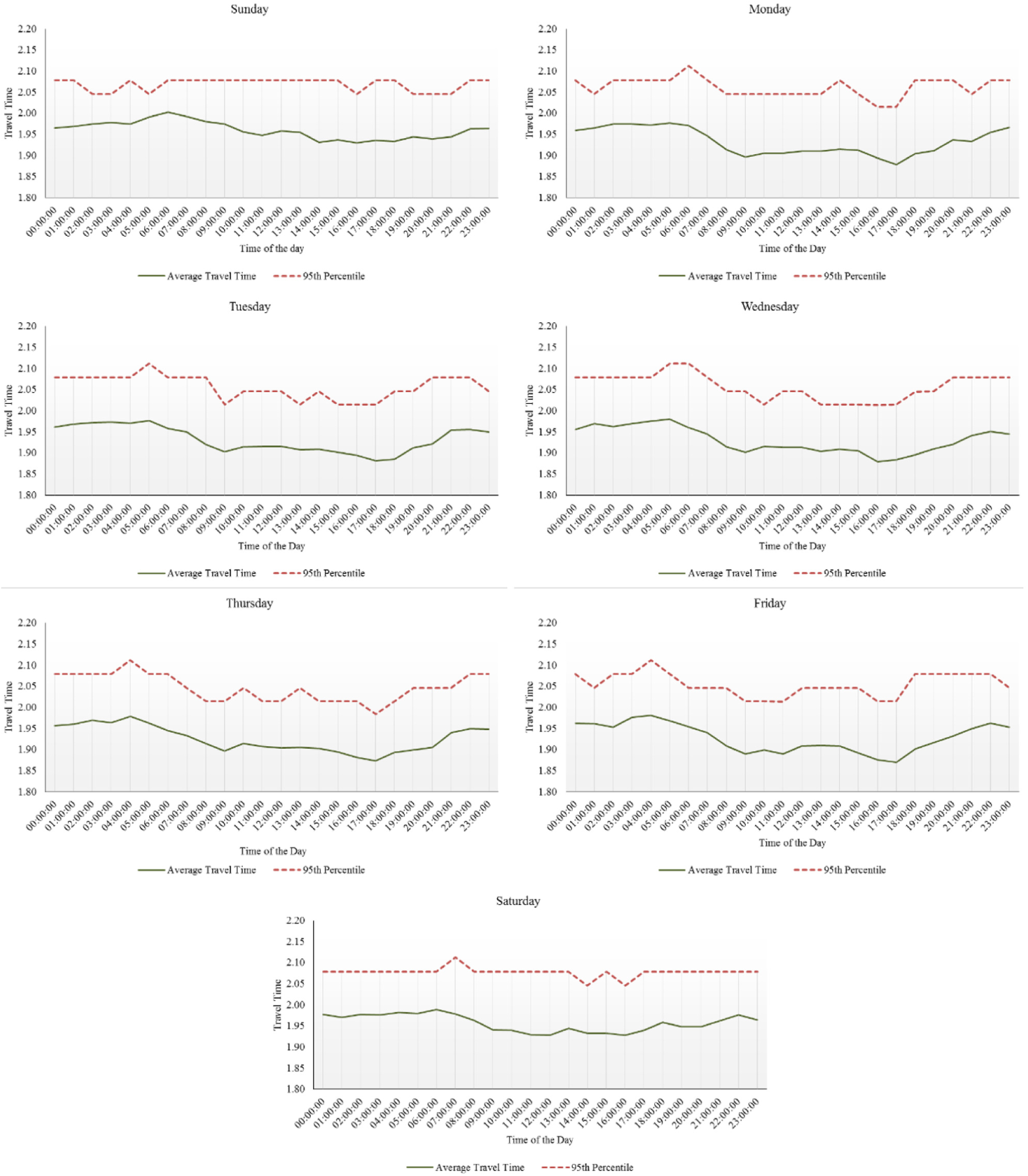
Segment that is unreliable during all times of the day and days of the week.
Figure 2 shows the comparison of the average travel time and the 95th percentile travel time for the 3.6-mi segment on I-77 northbound at the Gilead Road/Exit 23 intersection. From Figure 2, it can be noticed that the 95th percentile travel time is always equal to the average travel time, except during evening peak hours from Monday through Saturday. However, the 95th percentile travel time is equal to the average travel time during any time-of-the-day on Sundays. This indicates that the segment is unreliable only during evening peak hours from Monday through Saturday and completely reliable on Sundays.
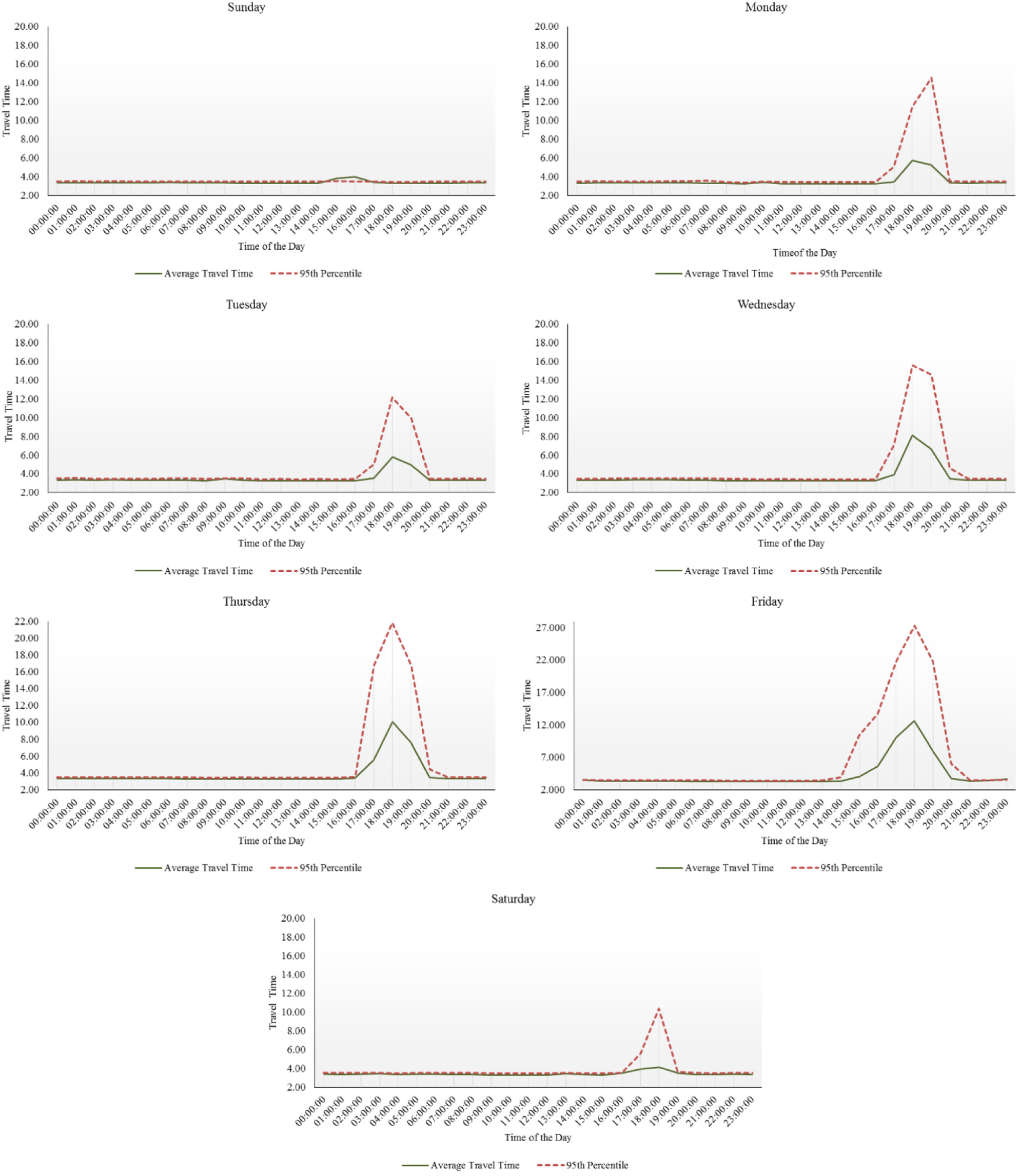
Segment that is unreliable during evening peak hours.
The reliability (total BT) of the link during a day-of-the-week can be evaluated by computing the area between the average travel time and 95th percentile travel time curves in Figures 1 and 2. For illustration, Figure 3 shows the area between the average travel time and the 95th percentile travel time for the 2.1-mi segment on I-77 northbound at the Harris Oak Boulevard/Reames Road/Exit 18 intersection on Mondays.
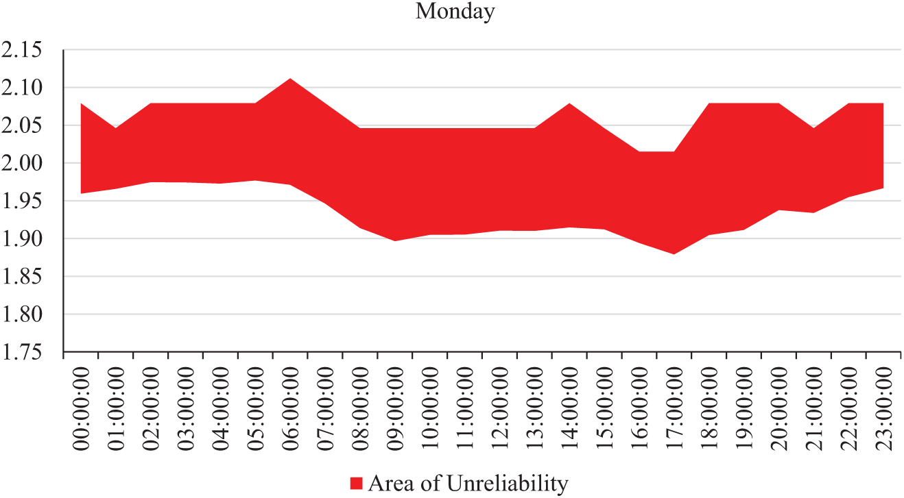
Area between average and 95th percentile travel time curves.
The BT between the curves during a peak hour (8:00 to 9:00 a.m.) is 15 s. Multiplying the BT with traffic volume between 8:00 and 9:00 a.m. (assume 6,000 vehicles) will give the total BT (1,500 min) during the considered peak period. Multiplying the total BT with the generalized value of reliability ($ 0.45 per minute) will help estimate the total value of unreliability ($600) during the considered peak hour. In case of availability of hourly traffic volumes for the entire day, the area in plots like Figure 3 with hourly traffic volumes on the x axis and BTs on the y axis will directly give the total BT for the time period considered. Multiplying the total BT with the generalized value of reliability will help monetize the value of reliability for the road segment considered by time-of-the-day and day-of-the-week.
Value of BT: Illustration
As discussed earlier, reliability accounts for consistency in travel times. Travelers account for the variability in the travel time and plan for BT along with the average travel time to their destination. The unreliability increases as the BT increases. The cost associated with the planned BT varies when compared with the travel time savings. For example, a traveler may plan for a BT of 15 min to his/her 25-min trip. The planned additional 15 min is because of the uncertainty in the travel time between the origin and destination (to ensure that he/she reaches a destination on time). As the uncertainty in the travel times on the road links between the origin and destination decreases, the planned BT will also decrease. The value of the planned BT is different when compared with the travel time savings for the 25-min trip. It also varies by time-of-the-day and day-of-the-week. The following example illustrates the use of the value of BT in estimating benefits.
Example: Estimating the Benefits from a Reliable Route
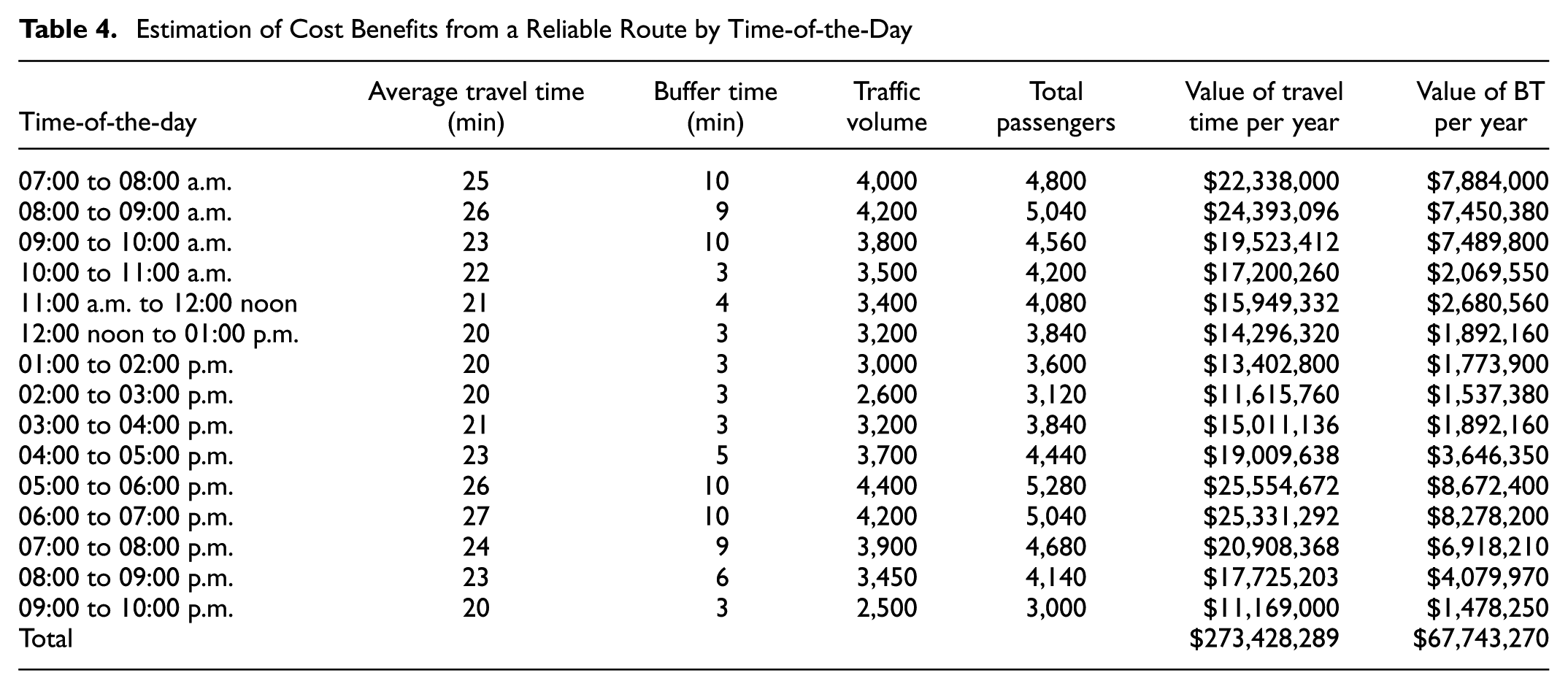
Consider a 10-mi road link with average travel times as presented in column 2 of Table 4. Column 3 is BT for each trip during the given hour. Similarly, the traffic volumes on the given road for each hour between 07:00 a.m. and 10:00 p.m. are shown in column 4. Column 5 shows the total passengers traveled with 1.2 as the average vehicle occupancy rate. Column 6 shows the value of travel time, and column 7 shows the value of BT. For this transportation project or alternative, the total value of travel time is $273,428,289 per year, whereas the total value of BT is $67,743,270 per year.
Estimation of Cost Benefits from a Reliable Route by Time-of-the-Day
Like the above example, a real-world scenario is considered to illustrate the value of reliability. For this purpose, widening of a 10.3-mi section from four lanes to six lanes on I-40 South of Trinity Road, Raleigh is considered. After widening the road, the difference between the maximum travel time (95th percentile travel time is not available for illustration) and the average travel time decreased from 9 min to 2 min during the morning peak hour. Similarly, the difference between the maximum travel time and the average travel time reduced from 10.5 min to 2.7 min during the evening peak hour.
The generalized value of BT is $ 0.45 per minute. The traffic volumes after completion of road widening are considered to evaluate the value of improved reliability from road widening. Table 5 shows the overall value of the project because of improved reliability during peak hours, on widening the I-40 section. A quick comparison with benefits created by a decrease in travel time for the same section indicates greater benefits achieved because of reduction in BT along this I-40 section.
Cost Benefits of Improved Reliability from Widening of I-40
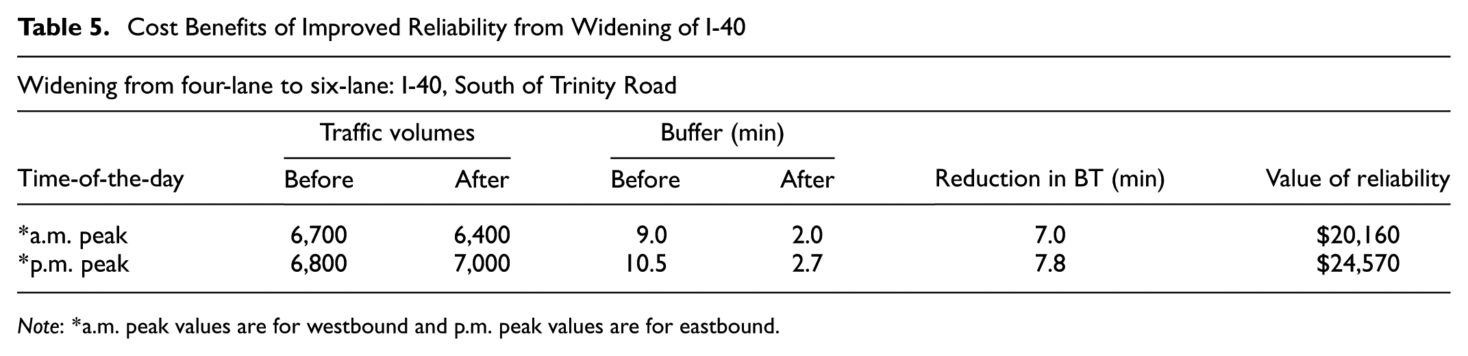
Note: *a.m. peak values are for westbound and p.m. peak values are for eastbound.
Conclusion
The average travel time and BT (difference between the 95th percentile travel time and the average travel time) are the performance measures that are considered for illustration to evaluate transportation projects or alternatives. This hourly data required for evaluation could be easily extracted from private data sources or other means. The monetary values for average travel time and BT are $ 0.51 and $ 0.45 per minute, respectively.
The illustration of the use of monetary values indicates that benefits achieved through reduction in BT are substantially higher compared with benefits from decrease in travel time for the same section. The illustration of use of monetary value of BT helps agencies in prioritizing transportation projects or alternatives. The processes help the agencies efficiently and effectively use the limited available resources.
The effect and impact of transportation projects or alternatives are monetized through illustrations to evaluate and make improved decisions. Both improved travel time and reliability on roads yield significant monetary benefits. However, greater benefits can be achieved through improved reliability compared with benefits from decrease in travel time for a given section of road.
The outcomes from this research to monetize reliability for evaluating the impact of transportation alternatives is completely based on the surveys obtained from passenger car users ( 20 ). Therefore, the illustrations presented in this paper are only applicable for evaluating the impact based on the value of travel time reliability for passenger cars. The findings are not applicable for other modes of travel or vehicle types (such as trucks).
There are many ways to address and reduce recurring and nonrecurring congestion. Only long-term solutions (such as construction projects) were considered for illustration purposes in this research. However, the illustrative approaches could be adopted or adapted to conduct assessments of other solutions and strategies (for example, freeway management patrols, incident management, etc.).
The illustrations presented in this paper are based on generalized values for the state of North Carolina. It is likely that tolerance levels and the value of reliability could vary based on the trip lengths (time or distance). Incorporating such variations in assessing the value of reliability merits an investigation.
Unreliable travel times for truckers could lead to late shipments and disruption of on-time delivery, resulting in loss of competitive edge over other shippers. Therefore, the value of travel time reliability for trucks could be very high compared with passenger car travel time reliability. Effective methods for evaluating travel time reliability for freight and monetizing reliability for trucks (freight transportation) also merit an investigation.
Footnotes
Acknowledgements
The authors acknowledge the NCDOT for providing financial support for this project. Special thanks are extended to J. Kevin Lacy, Kelly Wells, Dwayne Alligood, Cheryl Evans, Terry Hopkins, Ehren Meister, David Wasserman, A. Whitley IV, Terry Arellano, Joseph Geigle, Meredith McDiarmid, Alpesh Patel, Anthony Wyatt and Ernest Morrison of NCDOT for providing excellent support, guidance, and valuable inputs for successful completion of this project. In addition, data collection efforts by transportation engineering graduate students of the Department of Civil & Environmental Engineering at The University of North Carolina at Charlotte (UNC Charlotte) is also appreciated and recognized.
Author Contributions
The authors confirm contribution to each section of the paper. All the authors reviewed the results and approved the final version of the manuscript.
The Standing Committee on Transportation Programming and Investment Decision-Making (ADA50) peer-reviewed this paper (18-05371).
The contents of this paper reflect the views of the authors and not necessarily the views of the UNC Charlotte or the NCDOT. The authors are responsible for the facts and the accuracy of the data presented here. The contents do not necessarily reflect the official views or policies of either UNC Charlotte, NCDOT or the Federal Highway Administration (FHWA) at the time of publication. This paper does not constitute a standard, specification, or regulation.