Evaluation of Clustering Algorithms for the Prediction of Trends in Bus Travel Time

Abstract

Providing accurate and reliable travel time information to travellers is essential to improve the quality of public transit systems. With the availability of the latest technologies, it has become possible to collect a large amount of traffic data to analyze and understand these systems better. Traffic in India is characterized by lack of lane discipline and the presence of vehicles of varying static and dynamic characteristics, which makes prediction of bus travel time especially challenging. The aim of this study is to identify both a prediction algorithm that can handle high variability and suitable inputs or regressors to be used. Earlier studies performed offline manual grouping considering the patterns observed, which leads to limitations for automated field implementations. The present study explores the use of data-driven approaches, primarily clustering, to address the challenges for the prediction of bus travel time trends. Discrete wavelet transform (DWT) was used to extract trends from the travel time measurements. Three popular clustering algorithms—k-means, hierarchical, and self organizing maps (SOM)—were used to identify patterns. Travel time trends were then predicted by searching for similar cluster patterns within the historical database using pattern sequence-based forecasting (PSF). A comparison of the performance of these algorithms was carried out based on prediction errors. The clustering +prediction framework developed was also compared with the case when no clustering was done on the regressor dataset.

Travel time is one of the most popular measures of traffic system performance, as it can be easily perceived by users as well as by operators, planners, and researchers. Most of the private and public vehicles operating in metropolitan cities are now equipped with global positioning system (GPS) devices. Due to the low operation and maintenance costs associated with GPS devices, they are widely used for real-time tracking of vehicles such as public buses. In this process of tracking vehicles’ trajectories, a huge amount of trajectory data is generated which serves as a rich historical database. Many studies have reported on travel time prediction using GPS data from buses ( 1 – 3 ). In all these studies, however, a systematic method to identify the best inputs for the prediction process is lacking.

The accuracy of any prediction algorithm depends on the input provided to it. Hence, there is a need to identify correct inputs for the prediction algorithm by considering the natural groupings in the data and also the high variability in the system. Travel time, in general, follows certain patterns such as trip-wise, daily, weekly, monthly, and yearly, and they influence the selection of the correct regressor ( 4 – 7 ). In the majority of the earlier studies on bus travel time prediction, suitable regressors were selected manually offline, based on these patterns. However, for real-time implementations, there is a need for an automated method to analyze the data in order to identify the correct inputs, referred to as regressors here, to be used to predict bus travel times. For example, Kumar et al. ( 7 ) predicted travel times by identifying significant regressors using statistical analysis by considering each day of the week separately. The patterns were identified offline and were not dynamic in nature. However, in the real world these patterns may not be static and may vary depending on the day, time, location, etc. The system being very dynamic, a technique needs to be developed to group the data automatically rather than separating them manually using known patterns such as daily and/or weekly trajectories. Thus, there is a need to identify the correct regressors for the prediction algorithm by considering the natural groupings in the data and also the high variability in the system, ideally with an automated approach. Dynamic techniques need to be identified to do this grouping of data automatically rather than separating it manually using daily or weekly patterns. Clustering is one such data-driven, dynamic technique which can be used to identify the natural groups within a data set. This approach is possible if a large historical database is available. Once such groups are identified, the characteristics of the group can be used for better travel time prediction. For example, Van Der Voort et al. ( 8 ) predicted traffic flow on a motorway by dividing the data set manually into weekdays and weekends and also by clustering it using Kohonen maps. It was shown that the latter worked better than the case when the regressor dataset was divided manually.

The choice of the type of clustering technique to be used and the number of clusters into which the data should be divided are two major questions that should be answered. According to Jain et al. ( 9 ), there is no clustering technique that can be applied universally. Hence, the identification of the clustering technique that is best suited to the data is a major concern. The important clustering algorithms include: partitional, hierarchical, model-based, density-based, grid-based, and self organizing maps (SOM). Partitioning clustering algorithms, like k-means clustering, divide the dataset containing n unlabeled objects into k clusters such that each of the clusters formed has at least one object in it ( 10 , 11 ). However, the optimum value of k should be known. Hierarchical clustering ( 12 ) is another popular clustering algorithm which uses either agglomerative or divisive techniques to create a hierarchy of clusters. In a model-based clustering approach, the data is assumed to belong to a mixture of probability distributions, each representing a different cluster. It then finds the best fit of data to that model ( 13 ). SOM, or Kohonen maps ( 14 ), is a type of artificial neural network which projects higher dimensional data into a lower dimension (typically 2-D). Other popular clustering algorithms include density-based clustering ( 15 ) and grid-based clustering ( 16 ). However, parameters such as density thresholds ( 17 ) need to be defined and are not used for time series clustering due to high complexity ( 18 ).

Clustering techniques have been reported for prediction of traffic parameters. Chung ( 19 ) used a clustering algorithm to group historical travel time data. The computation time reduced significantly after the data was clustered, as only similar segments of the historical database need to be searched to identify the patterns. Ladino et al. ( 20 ) used a k-means clustering algorithm to organize a historical database into clusters and then used Kalman filtering technique to predict travel time for each cluster. Park et al. ( 21 ) used fuzzy c-means clustering and Kohonen SOM to cluster historical link travel times and calibrated individual artificial neural network (ANN) for each class. However, all these studies were limited to homogenous traffic conditions.

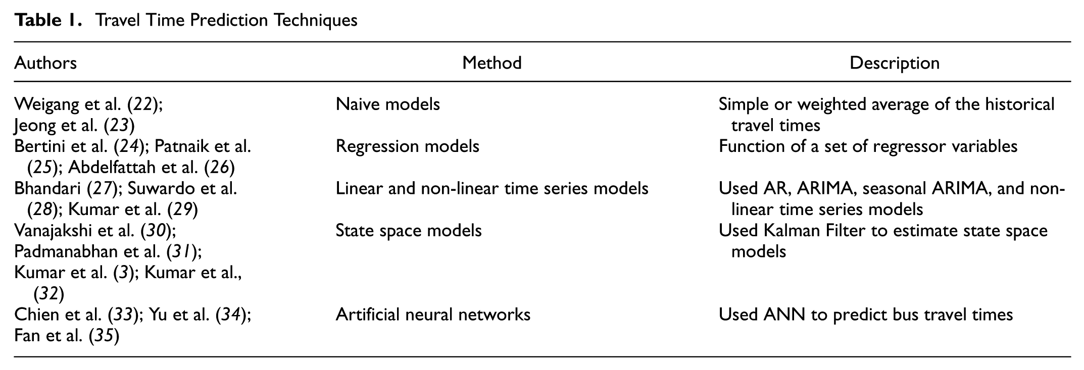
A detailed literature review on bus travel time prediction was carried out. The techniques used for travel time prediction can be categorized into naive models, regression models, linear and non-linear time series models, state space models, and ANN, as summarized in Table 1.

Table 1.

Travel Time Prediction Techniques

Authors	Method	Description
Weigang et al. ( 22 ); Jeong et al. ( 23 )	Naive models	Simple or weighted average of the historical travel times
Bertini et al. ( 24 ); Patnaik et al. ( 25 ); Abdelfattah et al. ( 26 )	Regression models	Function of a set of regressor variables
Bhandari ( 27 ); Suwardo et al. ( 28 ); Kumar et al. ( 29 )	Linear and non-linear time series models	Used AR, ARIMA, seasonal ARIMA, and non-linear time series models
Vanajakshi et al. ( 30 ); Padmanabhan et al. ( 31 ); Kumar et al. ( 3 ); Kumar et al., ( 32 )	State space models	Used Kalman Filter to estimate state space models
Chien et al. ( 33 ); Yu et al. ( 34 ); Fan et al. ( 35 )	Artificial neural networks	Used ANN to predict bus travel times

A prediction methodology was developed based on a pattern sequence-based forecasting (PSF) algorithm. The two main steps in PSF include the use of a suitable clustering technique to obtain cluster labels and prediction of future values by searching for the previous cluster labels within the database. Alvarez et al. ( 36 ) used PSF to predict future energy demand by clustering the data set using k-means. It was reported that this technique showed remarkable improvement compared with predictions made using autoregressive integrated moving average (ARIMA) or ANN. Jin et al. ( 37 ) extended energy demand forecasting using PSF technique, with SOM as the clustering technique. It was shown that PSF which used SOM as initial classifier worked better when compared with k-means as the initial classifier.

From the review of the literature, it was seen that not many studies which used clustering as a pre-processing tool for prediction involved mixed traffic conditions. In addition, in the majority of these studies, patterns in travel time were identified manually using chronological factors. There is a lack of an automated method for travel time prediction based on bus GPS data by identifying the trends in travel times. Considering these limitations, the present study aims to:

Identify natural groupings in the data using popular clustering techniques such as k-means, hierarchical, and SOM clustering.

Carry out the prediction of trends in travel time using PSF technique and compare the prediction performance using each of the clustering techniques.

Compare the performance of the clustering +prediction framework with the no clustering case.

Data Collection

The data used for the study were collected using GPS devices fixed to Metropolitan Transport Corporation buses in Chennai, the capital city of the state of Tamil Nadu, India. The 19B bus route was chosen as the study stretch. The route spans a length of 29.4 km and connects Kelambakkam, a suburban area of the city, to Saidapet, a major commercial area of the city. The northbound 19B route was chosen for the analysis. The GPS data were collected every 5 s from the GPS units fitted to the buses. Data were collected from a total of 1,024 trips during a period of 45 days. The obtained GPS data includes date, timestamp, and latitude and longitude of the bus location. The distance between two consecutive GPS points was calculated using the Haversine formula ( 38 ). For the purpose of analysis, the route was divided into 500-m sections, resulting in 56 sections. The travel times for each 500-m section were calculated using interpolation.

Preliminary Analysis

Travel times vary both spatially and temporally. In addition, travel times may follow yearly, monthly, weekly, daily, and hourly patterns. Many of these patterns are assumed to be recurrent in nature. Within a week, travel time patterns may differ between weekdays and weekends. Travel time also varies spatially and is affected by the characteristics of the area and the presence of signals, bus stops, and intersections. Based on all these, a data hierarchy structure of the travel time is prepared first and is shown in Figure 1. It can be seen from Figure 1 that the travel time data is high dimensional and varies with many factors.

Figure 1.

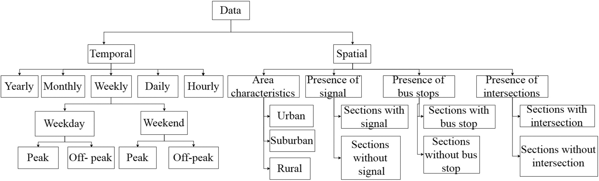
Data hierarchy.

To understand the variation of travel time in each section, the variance of travel time in each section was calculated using available data. Figure 2 shows the variance in travel times calculated for 500-m sections. It can be seen that the travel time along the study stretch is highly variable. The high peaks in the plot correspond to sections with bus stops and/or intersections. For example, the highest variance can be observed for section 47, a section near TIDEL Park, which is a major information technology park in Chennai. This section has a bus stop and two major intersections within 100 m distance. This causes delays, thereby increasing the travel times to a high value. It can also be seen that initial sections, such as section 10, have low travel time variance. The reason could be that these sections are located in the suburban area before the bus enters the city limits. Section 33 was taken as a representative sample section from within the city limits, but with no bus stops and/or intersections. It can be observed that the variance of travel time in this section is not as high as section 47, nor as low as section 10. These three sections were chosen as sample sections for further analyses, namely, section 10 for low travel time, section 33 for urban section with no bus stops or intersections, and section 47 for urban section with a bus stop and intersection.

Figure 2.

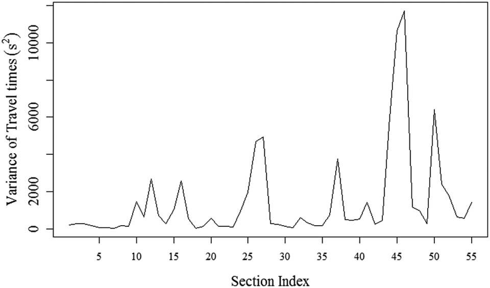
Variance in travel times for each section of route 19B.

Proposed Methodology

The proposed prediction methodology uses a PSF algorithm. This algorithm involves two main steps: clustering and prediction. The data is initially clustered and cluster labels are obtained. Further, the prediction is carried out based on the cluster labels. This method can be applied to predict travel times in a time series, either one-dimensional or multi-dimensional. Figure 3 shows the prediction framework used in this study. A detailed description of all the steps in the algorithm is provided in the following sections.

Figure 3.

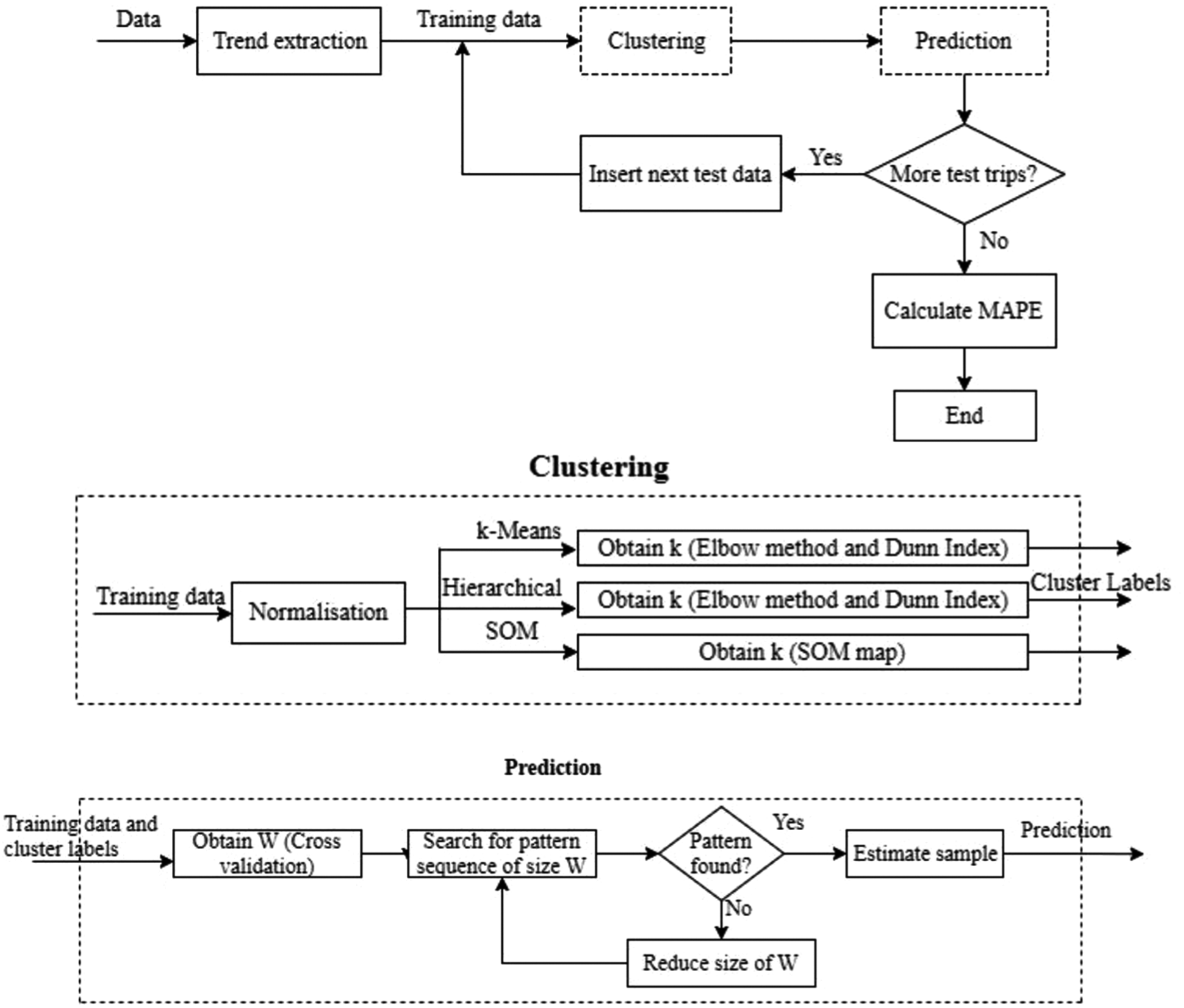
Proposed methodology of PSF.

Extraction of Travel Time Trends

A signal can be considered to be a combination of a trend component and a high-frequency component. The definition of trend is subjective based on the application. The trend, in general, can be defined as the predictable component of a signal, which will be predominantly the low-frequency part. It is the smoothened part of the signal and holds significant information contained in the signal. The travel time data under consideration is highly variable, consisting of both trends and high-frequency variations. In this study, the travel time trends extracted from the travel time measurements were used as regressors for prediction, while the high-frequency variations will be handled by a more sophisticated algorithm later.

Trends can be extracted from time series data using various techniques such as moving average filtering ( 39 ), median filtering ( 40 ), and discrete wavelet transforms (DWT) ( 41 ). Wavelet-based trend extraction was reported to be more efficient as it can reconstruct the signal without loss of much information ( 41 ). Hence, in this study, the trends in travel time were extracted using DWT. For this, the travel time data is first decomposed into wavelets at different levels of resolution. The wavelet coefficients at the lower levels of resolution were then thresholded using soft policy. In soft policy, the wavelet coefficients less than the threshold value are set to zero, whereas the threshold value is subtracted from those wavelet coefficients which are greater than the threshold. The threshold levels were chosen such that the trend extracted captures at least 70% of the signal. After thresholding, the signal is reconstructed. This reconstructed signal now contains the trends extracted.

Clustering

Clustering is a data-driven technique which can be used to find k clusters from the group of data such that objects belonging to the same cluster are similar and dissimilar to the objects in the other clusters. The type of clustering technique to be used and the number of clusters into which the data should be divided into are the two major questions that should be answered. From the literature review, it was seen that k-means, hierarchical, and SOM are three popular clustering techniques used to group highly varying data. Hence, these three clustering algorithms were chosen for further analysis. The travel time trends of each of the selected sections were clustered using k-means, hierarchical, and SOM separately and were used as regressors to the prediction. Based on the predictions made, performance analysis of the three clustering algorithms was done to identify the clustering technique suitable for each scenario.

The travel time trend data used for clustering was scaled to improve the convergence properties of the clustering algorithms ( 42 ). The optimum number of clusters (k) for each of the clustering algorithms needs to be determined. For k-means clustering and hierarchical clustering, many validation indices are available to find the optimum number of clusters. Out of these, two popular methods were chosen: elbow method ( 43 ), and Dunn index ( 44 ). For SOM, the number of optimum clusters (k) was identified from the U-Matrix ( 45 ). The optimum number of clusters k using k-means, hierarchical clustering, and SOM, respectively are: Section 10: {9, 5, 3}; Section 33: {9, 6, 4} and Section 47: {6, 6, 5}.

Pattern Sequence-Based Forecasting (PSF)

Given the travel time trends of a section up to trip d, our aim is to predict the travel time trend of the next trip d+1 for the same section. Let Y(i) be the travel time trend of the section for the i^th trip and C(i) €{1,…,k} be the cluster label for the i^th trip. Let S_wⁱ denote the sequence of cluster labels of the section travel time trend for W consecutive trips, from day i backward.

S_{W}^{i} = [C_{i - W + 1}, C_{i - W + 2}, \dots, C_{i}]

(1)

The prediction algorithm then searches for the sequence of labels of length S_W^d in the database to obtain the subsequence set $E S_{d + 1}$ .

E S_{d + 1} = {j such that S_{W}^{j} = S_{W}^{d}} .

(2)

In case no matching pattern is found, the value of W is reduced by 1 and the pattern search is again initiated. Once the pattern is identified, the predicted value of travel time trend for the next trip d+1 is obtained by averaging the travel time trends of the members in the set $E S_{d + 1}$ as:

\hat{Y} (d + 1) = \frac{1}{size (E S_{d + 1})} \sum_{j \in E S_{d + 1}} Y (j + 1),

(3)

where size( $E S_{d + 1}$ ) is the number of elements in the set $E S_{d + 1}$ . The process is repeated until all the test trips are predicted.

Determining the Number of Previous Trip Labels

The number of previous trip labels to be considered (W) for the PSF algorithm is another parameter that needs to be determined. The PSF algorithm searches the label sequence of W previous trips within the training data set in order to make a prediction. The value of W should be chosen such that the forecasting errors, as given in Equation 4, are minimized.

\sum_{d \in ts} ‖ \hat{Y} (d + 1) - Y (d + 1) ‖,

(4)

where $\hat{Y} (d + 1)$ is the predicted travel time trend of the(d+1)^th trip and Y(d+1) is the measured travel time trend of the (d+1)^th trip and ts denotes the training dataset. However, to find the value of $\hat{Y} (d + 1)$ , the members in the set $E S_{d + 1}$ should be known, which again depends on the value of W. Hence the value of W was found using cross-validation.

Cross-validation is the process of dividing a data set into a training data set for training the model and a test data set to evaluate the performance of the model ( 46 ). The traditional cross-validation can be applied only to data sets where the observations are independent. Hence, cross-validation is done on a rolling basis in this study ( 47 ). A 10-fold cross-validation is used for our study. The data set is divided into 10 partitions. In fold 1: partition [1] was used as training and partition [2] as the test set. In fold 2: partitions [1] and [2] were used as training and partition [3] was used as the test set. This process is repeated for all the folds. The mean absolute percentage error for cross-validation (MAPE_cv) was calculated for every fold, varying W. The average value of MAPE_cv (e_j) is then calculated for each window size by averaging across all 10 folds, as shown in Equation 5. W is selected as that value which minimizes the average value of MAPE_cv as shown in Equation 6.

e_{j} = \frac{1}{10} \sum_{i = 1}^{10} MAP E_{cv} {W = j},

(5)

W = \arg \min {e_{j}},

(6)

where j varies from 1 to W_max. Figure 4a, b and c below shows the sample plot of rolling cross-validation performed for travel time trends of section 47 using k-means, hierarchical, and SOM clustering, respectively. The values of W are chosen as 2, 1, and 1 for section 47 using k-means, hierarchical, and SOM clustering, respectively. A similar analysis was done for sections 10 and 33. The value of W obtained using k-means, hierarchical, and SOM clustering, respectively, are: Section 10: {3, 1, 1}; Section 33: {1, 2, 1} and Section 47: {2, 1, 1}.

Figure 4.

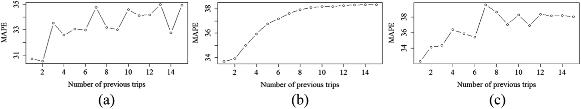
W for section 47 using (a) k-means, (b) hierarchical, and (c) SOM clustering.

Performance Evaluation

The PSF algorithm was implemented for each of the sections using the optimum number of clusters (k) and number of previous trip labels (W) obtained, as discussed above. The performance accuracy of each of the clustering algorithms for each section was quantified using mean absolute percentage error (MAPE) as follows:

MAPE = \frac{1}{n} \sum_{i = 1}^{n} \frac{| \hat{Y} - Y_{m} |}{Y_{m}} 100,

(7)

where $\hat{Y}$ is the predicted value of travel time trend, Y_m is the corresponding measured travel time trend, and n is the number of observations in the test data set. Figure 5a, b , and c show the measured versus the predicted travel time trends of section 10 using k-means, hierarchical, and SOM clustering. It can be seen that k-means works better for this section, which had low variance in travel times. Both hierarchical and SOM fail to capture the variations for the low variance section.

Figure 5.

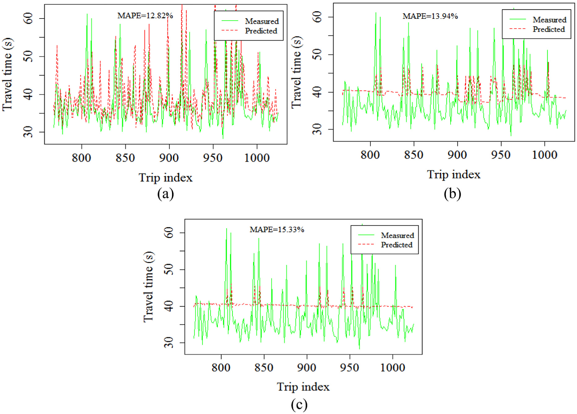
Measured and predicted travel time trends of section 10 using (a) k-means, (b) hierarchical, and (c) SOM clustering.

Figure 6 shows the measured versus the predicted travel time trends for section 33, which is an urban section without any signals or intersections. It can be seen that k-means also works best in this case, capturing the variations in travel time trends better than the other methods. Hierarchical clustering gives poor performance in this case too, whereas the performance of SOM has improved.

Figure 6.

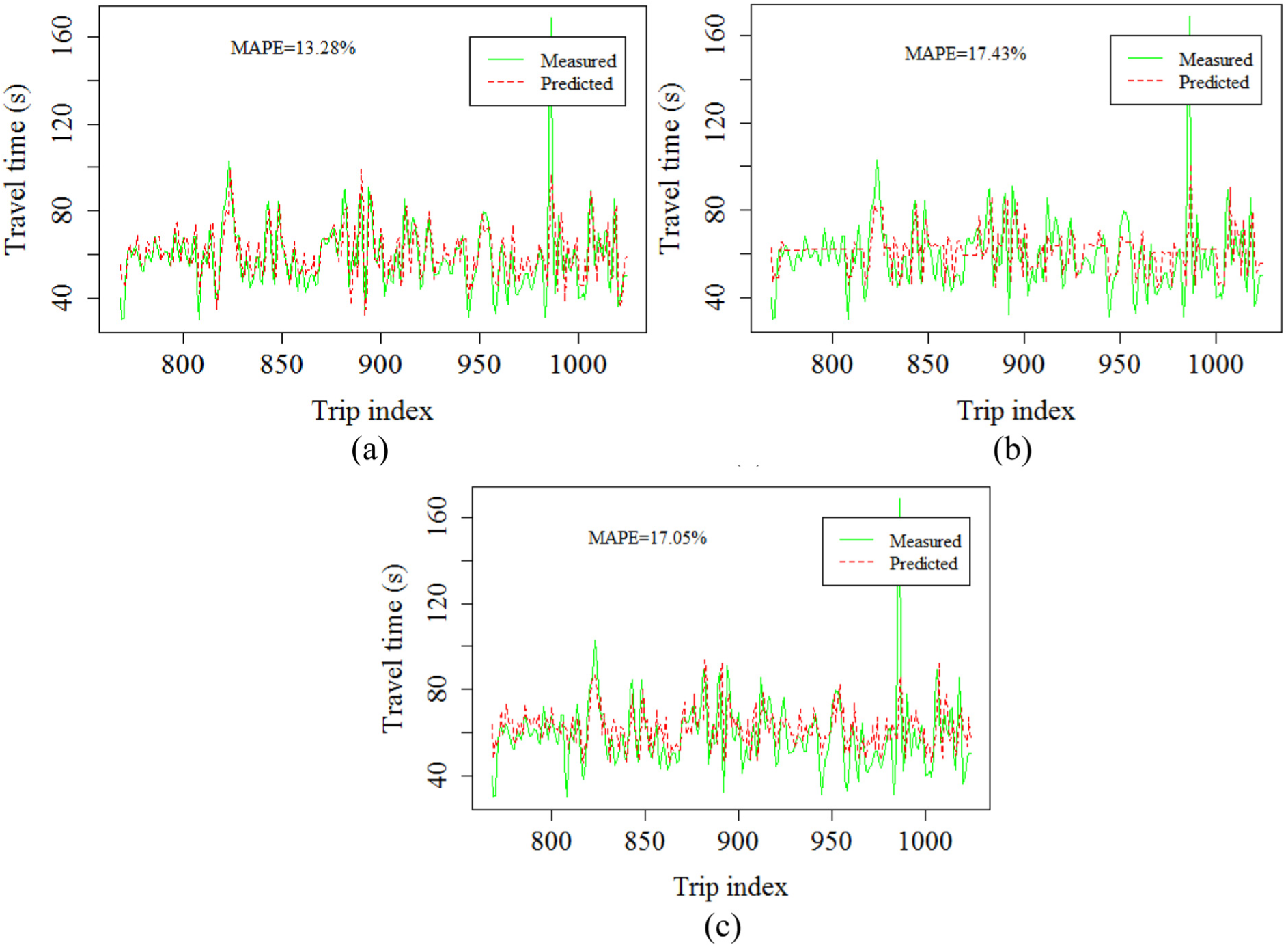
Measured and predicted travel time trends of section 33 using (a) k-means, (b) hierarchical, and (c) SOM clustering.

Figure 7 shows the results for section 47, which is the section with the highest variance in travel times along the selected route. It can be seen that the predictions based on k-means clustering work best, yielding a low value of MAPE and also capturing the variations in travel time trends. The predictions based on hierarchical clustering remain poor, whereas those based on SOM have improved. Hence it was concluded that k-means works best for all the sections under study. The trend predictions based on hierarchical clustering remain poor in all three cases, whereas the performance of SOM improves as the section variance increases.

Figure 7.

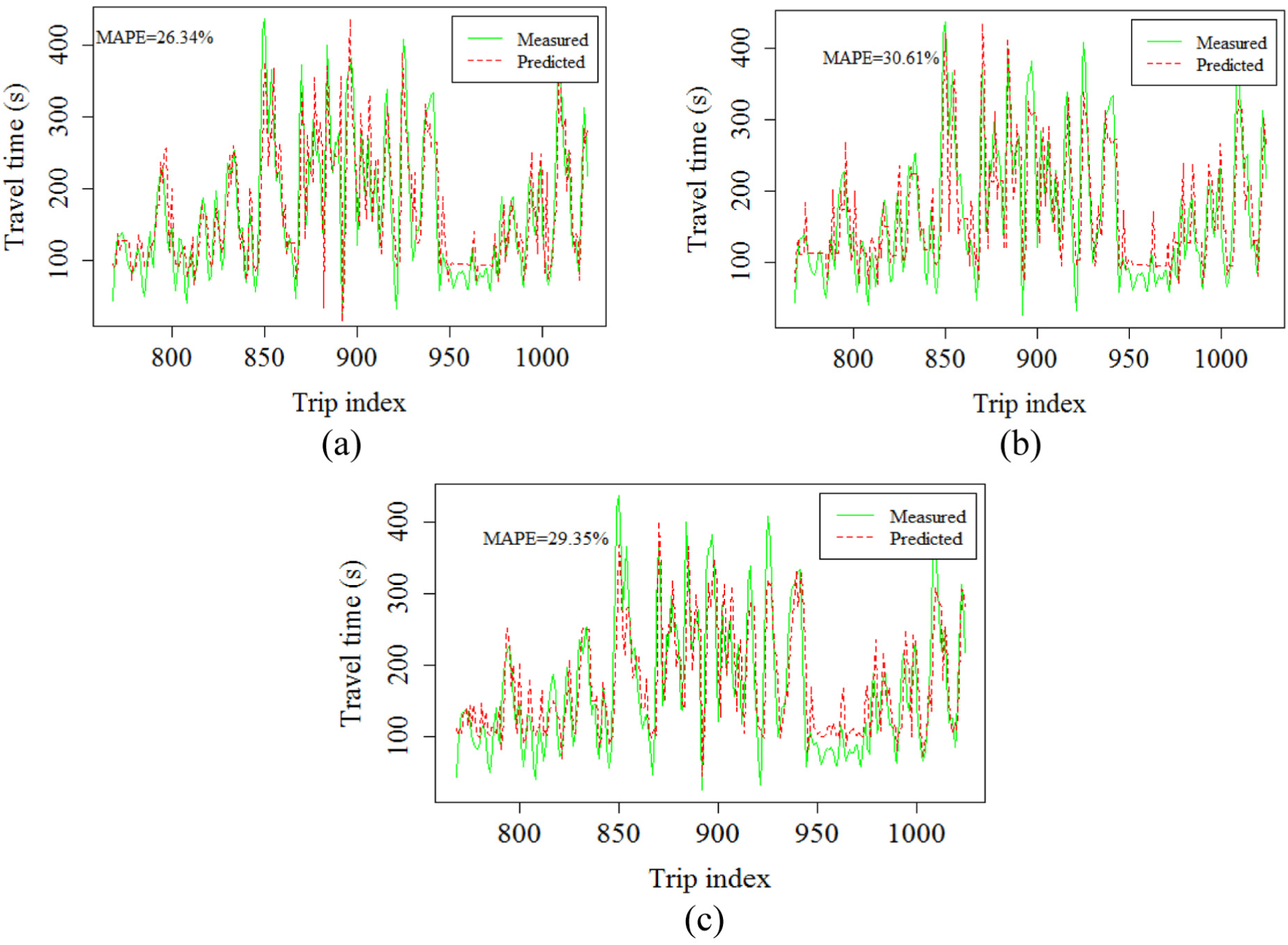
Measured and predicted travel time trends of section 47 using (a) k-means, (b) hierarchical, and (c) SOM clustering.

Clustering prior to prediction helps to improve the prediction accuracy. The results of the clustering + prediction framework obtained using the PSF algorithm were compared with the case when no clustering was done. In the no clustering case, predictions were obtained by taking the average of the previous W travel time trends of the same section. Figure 8 shows the comparison between the predictions made using the PSF algorithm and the no clustering case for a sample section on the seven days in the test dataset. It can be seen that, in all the cases, the MAPE obtained using clustering + PSF algorithm was lower compared with the no clustering case, indicating that the clustering helped to improve the prediction accuracy.

Figure 8.

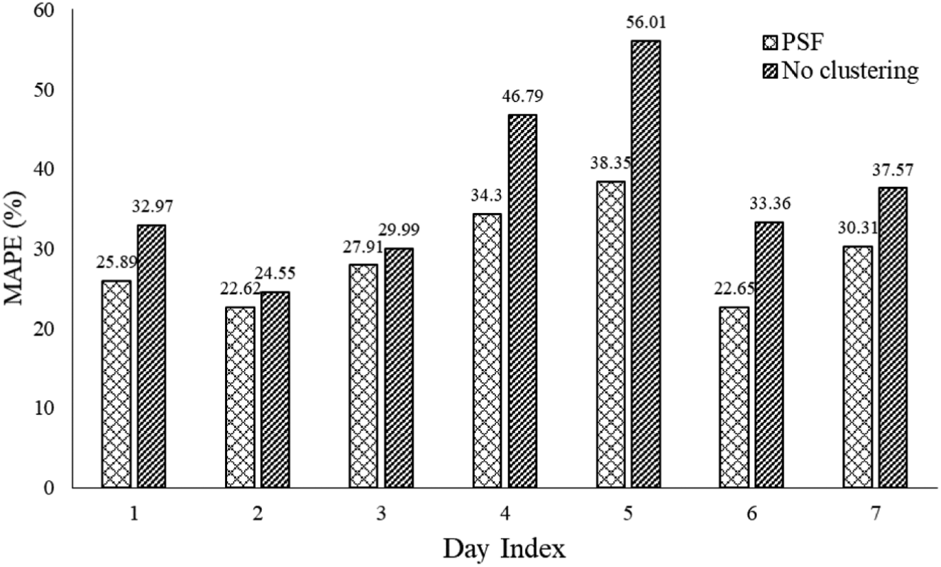
MAPE obtained for all days using PSF algorithm and no clustering case.

Summary and Conclusion

Travel time is a highly variable quantity, which depends on many factors, such as road conditions, weather conditions, driver behavior, etc. Addressing the high variability in travel time is a challenging task. Travel time prediction becomes even more complex in mixed traffic conditions, such as those prevailing in India. The present study identifies the proper regressors to be used for prediction of travel time trends, by comparing the performance of three popular clustering techniques—k-means, hierarchical, and SOM—for road sections with different characteristics. The following conclusions were drawn from the study:

Due to the high variability in travel time, manually grouping travel times into weekdays, weekends, or day-wise is not a very efficient method. Data-driven techniques such as clustering can be used to identify the natural groupings in the data automatically. This becomes possible with the availability of huge amounts of historical data from automated sensors.

A clustering + prediction framework was developed using a PSF algorithm to predict travel time trends. It was seen that, for all the three sections with different characteristics which were analyzed, PSF based on k-means clustering performed well. The performance of hierarchical clustering remained poor in all the cases, whereas PSF based on SOM was able to capture the variations more effectively as the variation in travel time trends increased. In the later stages of the study, when the dimensionality of the regressor data increases, predictions based on k-means may not be efficient. In this case, clustering techniques which work efficiently with high dimensional data such as SOM might be required.

The clustering + prediction framework developed was compared with the case when no clustering was done. It was seen that predictions based on PSF yielded low MAPE value when compared with the case when no clustering was performed on the regressor dataset. Hence it was concluded that clustering prior to prediction helps to improve the accuracy of the prediction.

Footnotes

Acknowledgements

The authors acknowledge the Centre of Excellence in Urban Transport, IIT Madras, for the data collection.

Author Contributions

The authors confirm contribution to the paper as follows: study conception and design: Hima Elsa Shaji, Arun K. Tangirala, and Lelitha Vanajakshi; data collection: Shaji and Vanajakshi; analysis and interpretation of results: Shaji, Tangirala, and Vanajakshi; draft manuscript preparation: Shaji, Tangirala, and Vanajakshi. All authors reviewed the results and approved the final version of the manuscript.

The Standing Committee on Artificial Intelligence and Advanced Computing Applications (ABJ70) peer-reviewed this paper (18-05451).

References

Zhang

Xiao

Chen

Bus Arrival Time Prediction Based on GPS Data. Proc., 4th International Conference on Transportation Engineering, ICTE 2013, China, American Society of Civil Engineers, 2013, pp. 1470–1475.

Bin

Zhongzhen

Baozhen

Bus Arrival Time Prediction Using Support Vector Machines. Journal of Intelligent Transportation Systems, Vol. 10, No. 4, 2006, pp. 151–158.

Kumar

S. V.

Vanajakshi

Subramanian

S. C.

A Model Based Approach to Predict Stream Travel Time Using Public Transit as Probes. Proc., 2011 IEEE Intelligent Vehicles Symposium (IV), Baden-Baden, Germany, IEEE, New York, 2011, pp. 101–106.

Kwon

Coifman

Bickel

Day-to-Day Travel-Time Trends and Travel-Time Prediction from Loop-Detector Data. Transportation Research Record: Journal of the Transportation Research Board, 2000. 1717: 120–129.

Vlahogianni

E. I.

Karlaftis

M. G.

Golias

Kourbelis

Pattern-Based Short-Term Urban Traffic Predictor. Proc., 2006 IEEE Intelligent Transportation Systems Conference, Toronto, Ontario, Canada, IEEE, New York, 2006, pp. 389–393.

Kumar

S. V.

Vanajakshi

Pattern Identification Based Bus Arrival Time Prediction. Proc., Institution of Civil Engineers-Transport, Vol. 167, No. 3, Thomas Telford Ltd., 2014, pp. 194–203.

Kumar

B. A.

Vanajakshi

Subramanian

S. C.

Pattern-Based Bus Travel Time Prediction under Heterogeneous Traffic Conditions. Presented at 93rd Annual Meeting of the Transportation Research Board, Washington, D.C., 2014.

Van Der Voort

Dougherty

Watson

Combining Kohonen Maps with ARIMA Time Series Models To Forecast Traffic Flow. Transportation Research, Vol. 4, No. 5, 1996, pp. 307–318.

Jain

A. K.

Murty

M. N.

Flynn

P. J.

Data Clustering: A Review. ACM Computing Surveys (CSUR), Vol. 31, No. 3, 1999, pp. 264–323.

10.

Macqueen

Some Methods for Classification and Analysis of Multivariate Observations. Proceedings of the Fifth Berkeley Symposium on Mathematical Statistics and Probability, Vol. 1, No. 233, 1967, pp. 281–297.

11.

Bradley

P. P. S.

Fayyad

Reina

Scaling Clustering Algorithms to Large Databases. Proc., 4th International Conference on Knowledge Discovery and Data Mining. AAAI Press, New York, 1998, pp. 9–15.

12.

Kaufman

Rousseeuw

P. J.

Finding Groups in Data: An Introduction to Cluster Analysis. John Wiley & Sons, Inc., Vol. 344, New Jersey, 2009. http://dx.doi.org./10.1002/9780470316801

13.

Shavlik

J. W.

Dietterich

T. G.

Readings in Machine Learning. Morgan Kaufmann, Inc., San Mateo, California, 1990.

14.

Kohonen

The Self-Organizing Map. Proceedings of the IEEE, Vol. 78, No. 9, 1990, pp. 1464–1480.

15.

Ester

Kriegel

H. P.

Sander

A Density-Based Algorithm for Discovering Clusters in Large Spatial Databases with Noise. Knowledge Discovery and Data Mining, Vol. 96, No. 34, 1996, pp. 226–231.

16.

Grabusts

Borisov

Using Grid-Clustering Methods in Data Classification. Proc., International Conference on Parallel Computing in Electrical Engineering, PARELEC 2002, Warsaw, Poland, IEEE, New York, 2002, pp. 425–426.

17.

Gan

Data Clustering: Theory, Algorithms, and Applications. ASA-SIAMSeries on Statistics and Applied Probability, Vol. 20, Philadelphia, 2007.

18.

Aghabozorgi

Seyed Shirkhorshidi

Ying Wah

Time-Series Clustering – A Decade Review. Information Systems, Vol. 53, 2015, pp. 16–38.

19.

Chung

Classification of Traffic Pattern. Proc., 11th World Congress on ITS, Chicago, 2003, pp. 687–694.

20.

Ladino

Kibangou

Fourati

De Wit

C. C.

Travel Time Forecasting from Clustered Time Series via Optimal Fusion Strategy. Proc., 2016 European Control Conference, ECC 2016, Aalborg, Denmark, IEEE, New York, 2017, pp. 2234–2239.

21.

Park

Rilett

Forecasting Multiple-Period Freeway Link Travel Times Using Modular Neural Networks. Transportation Research Record: Journal of the Transportation Research Board, 1998. 1617: 163–170.

22.

Weigang

Koendjbiharie

de M Juca

R. C.

Yamashita

MacIver

Algorithms for Estimating Bus Arrival Times Using GPS Data. Proc., IEEE 5th International Conference on Intelligent Transportation Systems, Singapore, IEEE, New York, 2002, pp. 868–873.

23.

Jeong

Rilett

The Prediction of Bus Arrival Time Using AVL Data. Presented at 83rd Annual Meeting of the Transportation Research Board, Washington, D.C., 2004.

24.

Bertini

R. L.

El-Geneidy

A. M.

Modeling Transit Trip Time Using Archived Bus Dispatch System Data. Journal of Transportation Engineering, Vol. 130, No. 1, 2004, pp. 56–67.

25.

Patnaik

Chien

Bladikas

Estimation of Bus Arrival Times Using APC Data. Journal of Public Transportation, Vol. 7, No. 1, 2004, p. 1.

26.

Abdelfattah

A. M.

Khan

A. M.

Models for Predicting Bus Delays. Transportation Research Record, Journal of the Transportation Research Board, 1998. 1623: 8–15.

27.

Rajbhandari

Bus Arrival Time Prediction Using Stochastic Time Series and Markov Chains. Ph.D. thesis, New Jersey Institute of Technology, Newark, New Jersey, 2004.

28.

Suwardo

Napiah

Kamaruddin

ARIMA Models for Bus Travel Time Prediction. Journal of the Institute of Engineers Malaysia, Vol. 71, No. 2, 2010, pp. 49–58.

29.

Kumar

S. V.

Vanajakshi

Short-Term Traffic Flow Prediction Using Seasonal ARIMA Model with Limited Input Data. European Transport Research Review, Vol. 7, No. 3, 2015, pp. 1–9.

30.

Vanajakshi

Subramanian

S. C.

Sivanandan

, R. Travel Time Prediction Under Heterogeneous Traffic Conditions Using Global Positioning System Data from Buses. IET Intelligent Transport Systems, Vol. 3, No. 1, 2009, pp. 1–9.

31.

Padmanaban

R. P. S.

Vanajakshi

Subramanian

S. C.

Estimation of Bus Travel Time Incorporating Dwell Time for APTS Applications. Proc., 2009 IEEE Intelligent Vehicles Symposium, Xi’an, China, IEEE, New York, 2009, pp. 955–959.

32.

Kumar

B. A.

Vanajakshi

Subramanian

S. C.

Bus Travel Time Prediction Using a Time-Space Discretization Approach. Transportation Research Part C: Emerging Technologies, Vol. 79, 2017, pp. 308–332.

33.

Chien

S. I. J.

Ding

Wei

Dynamic Bus Arrival Time Prediction with Artificial Neural Networks. Journal of Transportation Engineering, Vol. 128, No. 5, 2002, pp. 429–438.

34.

Yang

Z. Z.

Chen

Hybrid Model for Prediction of Bus Arrival Times at Next Station. Journal of Advanced Transportation, Vol. 44, No. 3, 2010, pp. 193–204.

35.

Fan

Gurmu

Dynamic Travel Time Prediction Models for Buses Using only GPS Data. International Journal of Transportation Science and Technology, Vol. 4, No. 4, 2015, pp. 353–366.

36.

Alvarez

F. M.

Troncoso

Riquelme

J. C.

Ruiz

J. S. A.

Energy Time Series Forecasting Based on Pattern Sequence Similarity. IEEE Transactions on Knowledge and Data Engineering, Vol. 23, No. 8, 2011, pp. 1230–1243.

37.

Jin

C. H.

Pok

Lee

Park

H. W.

Kim

K. D.

Yun

Ryu

K. H.

A SOM Clustering Pattern Sequence-Based next Symbol Prediction Method for Day-Ahead Direct Electricity Load and Price Forecasting. Energy Conversion and Management, Vol. 90, 2015, pp. 84–92.

38.

Chamberlain

Great Circle Distance between Two Points. 2014. http://www.movable-type.co.uk/scripts/gis-faq-5.1.html.

39.

Alvarez-Ramirez

Rodriguez

Echeverría

J. C.

Detrending Fluctuation Analysis Based on Moving Average Filtering. Physica A: Statistical Mechanics and its Applications, Vol. 354, 2005, pp. 199–219.

40.

Fried

Einbeck

Gather

Weighted Repeated Median Smoothing and Filtering. Journal of the American Statistical Association, Vol. 102, No. 480, 2007, pp. 1300–1308.

41.

Dash

Maurya

M. R.

Venkatasubramanian

Rengaswamy

A Novel Interval-Halving Framework for Automated Identification of Process Trends. American Institute of Chemical Engineers Journal, Vol. 50, No. 1, 2004, pp. 149–162.

42.

Neuristique

L. B.

Bengio

Convergence Properties of the K-Means Algorithms. Proc., 7th International Conference on Neural Information Processing Systems, Denver, Colo., MIT Press, Cambridge, Mass., 1995, pp. 585–592.

43.

Thorndike

R. L.

Who Belongs in the Family?

Psychometrika, Vol. 18, No. 4, 1953, pp. 267–276.

44.

Dunn

J. C.

Well-Separated Clusters and Optimal Fuzzy Partitions. Journal of Cybernetics, Vol. 4, No. 1, 1974, pp. 95–104.

45.

Ultsch

Self-Organizing Neural Networks for Visualization and Classification. In Information and Classification ( Opitz

Lausen

Klar

, eds.), Springer-Verlag, Berlin, 1993, pp. 307–313.

46.

Kohavi

A Study of Cross-Validation and Bootstrap for Accuracy Estimation and Model Selection. Proc., International Joint Conference on Artificial Intelligence (IJCAI), Canada, Morgan Kaufmann, Inc., California, Vol. 5, 1995, pp. 1–7.

47.

Arlot

Celisse

A Survey of Cross-Validation Procedures for Model Selection. Statistics Surveys, Vol. 4, 2010, pp. 40–79.