Modeling Free-flow Speeds on Undivided Roads in Mixed Traffic with Weak Lane Discipline

Abstract

In developing countries like India, transportation systems are characterized by limited roadway infrastructure and lack of operation and management experience. Hence, there exists a need to evaluate a performance indicator that reflects the current level of service (LOS) of a road facility. Free-flow speed (FFS) is a key parameter used to express LOS assessment. The objective of this study is to develop FFS prediction models for undivided roads with mixed traffic conditions in both urban and rural settings in India. Traffic data were collected from two-way two-lane undivided roads in southern India during free-flow traffic conditions using videographic method. Various class-specific and site-specific characteristics, such as vehicle class, subclass, carriageway width, link length, number of side roads, lateral clearance, land use type, and area type, were investigated and their influence on FFS evaluated. Statistical tests assessed the variations of obtained FFS with different vehicle-specific and site-specific factors. Free-flow prediction models were developed using linear regression method. The developed models show that FFS increases with greater carriageway width, lateral clearance, and link length, and decreases with increase in number of side roads. In general, FFS is higher in rural areas than urban areas. Similarly, open areas have higher FFS than residential, institutional, and commercial areas. The model can be used to predict FFS of undivided roads if site-specific and vehicle-specific data are known. This study finds interesting applications in capacity and LOS analysis, accident analysis, and before-and-after studies of road improvement schemes.

Free-flow speed (FFS) can be defined as the desired average speed adopted by a driver when not restricted by other vehicles in the traffic stream under a given set of road conditions. FFS is an important parameter that should be measured accurately in the field because it plays a major role in planning, operational analysis, and performance evaluation of transportation systems. However, field determination of FFS is resource intensive because it requires measuring a sufficient sample size of vehicle speeds at the appropriate time of low vehicle interaction and in appropriate locations with comparable geometric features. To overcome the challenges of field data collection, most highway agencies use modeling techniques to predict FFS.

In developing countries like India, trafﬁc is composed of a wide variety of different types of vehicles, such as cars, buses, trucks, light commercial vehicles, two-wheelers, three-wheelers, etc. These vehicles generally do not follow lane discipline and they occupy any position in the available road space. This type of traffic is known as mixed or heterogeneous traffic conditions. It is believed that different classes of vehicles have different speed values based on their size and characteristics. FFS also depends on site-specific characteristics such as land use, area type, roadway geometry, etc. In a literature review, it was found that the majority of studies on FFS are based on homogeneous traffic conditions. Studies on FFS under mixed traffic conditions are limited and these studies have been done mostly on divided roads. Also, not much attention has been given to site-specific characteristics in earlier studies. Hence, the main objective of the present study is to develop FFS prediction models for undivided roads under mixed traffic conditions with the following specific objectives:

To analyze whether FFS are statistically similar for different vehicle types and site-specific factors.

To study the influence on FFS of vehicle-specific and site-specific characteristics.

To develop overall and class-wise FFS prediction models for undivided roads under non-lane based mixed traffic conditions.

The rest of the paper is structured as follows: the next section focuses on a detailed review of the literature on FFS studies. The third section discusses the data collection and extraction process. The fourth section presents the results of analysis of FFS based on vehicle-specific and site-specific characteristics. FFS prediction models are presented in the fifth section, followed by a summary and conclusions.

Literature Review

FFS is defined as the average speed of a vehicle on a given facility, measured under low-volume conditions, when drivers tend to drive at their desired speed and are not constrained by control delay. The definitions of FFS given by the Highway Capacity Manual 2010 ( 1 ) are:

The theoretical speed when density and flow rate on a study segment are both zero.

The prevailing speed on freeways at flow rates of between 0 and 1,000 passenger cars per hour per lane (pc/h/ln)

Bang ( 2 ) studied the effect of side friction factors like carriage width, presence of shoulder or kerbs, shoulder width, side friction events, roadside land use, etc. on FFS. It was found that the impact of side friction was severe on FFS for both two-lane undivided roads, both interurban and urban.

Dixon et al. ( 3 ) quantified the relationship between posted speed limit and observed FFS on rural multilane highways. Some of the issues evaluated in that study include influence on FFS of: heavy vehicles, traffic volumes, access point density, and vertical grade. Ye et al. ( 4 ) also explored the effect of truck percentage, speed limit (65 and 55 miles/h), land use type (rural/urban), road classification (freeway/non-freeway), and number of lanes (four/six). The results show that vehicles in rural areas had higher FFS than in urban areas for all models, and vehicles on freeways had higher speed than on non-freeways. Kyte et al. ( 5 ) studied the effect of environmental factors on FFS. Data was collected using sensors which measured traffic, visibility, roadway, and weather data. The study concluded that wind speed, low lighting, and snow reduce driver speed. Hablas ( 6 ) attempted to quantify the impact of inclement weather (precipitation and visibility) on FFS of traffic stream along freeway sections. Wang ( 7 ) conducted a study to examine the relationship between FFS and posted speed limits on expressways in Beijing, China. A regression model was built to establish a relationship between 85th percentile speed and posted speed limit. Hashim ( 8 ) investigated the relationship between 85th percentile speed and headway to define a headway value corresponding to free moving vehicles. He found that the 85th percentile speed took a constant value at headway equal to five seconds or more. Azai and Vien ( 9 ) studied the factors affecting FFS on multilane highways in Malaysia. Further investigation on lane width, shoulder width, and access point was also done. Moses and Mtoi ( 10 ) developed FFS equations for urban arterials in Tallahassee, Florida, and compared the efficacy of models with the HCM 2010 ( 1 ) and Florida Department of Transportation methods. Wang et al. ( 11 ) developed a linear regression model to estimate FFS on freeways in California in order to investigate the impact of changes in pavement roughness on driving behavior with respect to speed. Andrade et al. ( 12 ) used multivariate analysis techniques to investigate the effect on FFS of posted speed, road class, number of lanes, access point density, geometric design, and roadside environment. Ma et al. ( 13 ) found that variance in FFS across study sections increased with increase in lane width at midblock, but did not show any significant impact at the exits of intersections. Tunde ( 14 ) used regression analysis to find the relationship between various factors (driver, vehicle, road geometry, and environment) and FFS on urban arterials in Nigeria. Tseng et al. ( 15 ) investigated the characteristics of FFS in relation to vehicle type, geometric design, and speed limit. Puan and Abdurrahman ( 16 ) made a comparison of FFS estimates obtained using moving car observer method with the Malaysian Highway Capacity Manual. Balakrishnan and Sivanandan ( 17 ) studied the influence on FFS of lane and vehicle subclass for urban roads in mixed traffic. Analysis of FFS was performed for all the vehicle-specific and site-specific factors. FFS prediction models were developed using multiple linear regression method, and multinomial logistic regression was employed for developing lane choice models. Rao and Rao ( 18 ) developed a model for FFS obtained in urban arterials of Delhi and compared it with the FFS obtained from developed and HCM 2010 ( 1 ) models. They found that the FFS value given by HCM 2010 ( 1 ) is higher than the field value. Yusuf et al. ( 19 ) performed statistical analysis and found that the environment, pedestrians, and roadway geometry have negative influences on FFS.

Speed and travel time studies are necessary for the determination of road performance. The literature review confirms that researchers have conducted studies on FFS to understand driving behavior and factors affecting it. These factors are generally related to drivers, roadway geometry, and land use. It is notable that the majority of the studies on FFS are based on homogeneous traffic conditions. Studies on FFS under mixed traffic conditions are limited in number. It was found that most of the factors influencing FFS in homogeneous traffic are applicable to mixed traffic also. However, it is evident that the presence of various vehicle groups is an important determining factor in mixed traffic conditions. Studies available for undivided road stretches with mixed traffic conditions are limited. Hence, it is necessary to develop a model for predicting the FFS of undivided roads, which are predominant in most of the rural and urban road network of India.

Data Collection and Extraction

In order to study and model the FFS on undivided roads, ten study sections were selected on various road stretches located in southern cities of India: Mangalore, Kannur, and Alappuzha. Traffic data were collected using videographic technique from all the chosen sites. The collected data were classified into following two groups:

Vehicle-specific data

Vehicle class and subclass

Number of vehicles (vehicles moving in both directions)

Site-specific data

Carriageway width

Link length

Side clearance

Number of side roads (roads which perpendicularly merge with the study stretch)

Land use (residential, institutional, commercial, and open)

Area type (rural, suburban, and urban)

The video data were collected from each site using a pair of camcorders for 1.5 hours which were synchronised for time. The data collection was done during the early morning hours, that is, between 5:30 am and 7:30 am, depending on the traffic flow rate, in order to observe free-flow conditions. The details of link length, geometric details, number of observations, and site-specific characteristics are shown in Table 1.

Table 1.

Site-Specific Details of Study Sections

Site no.	Site	Link length(m)	Distance between cameras(m)	CW(m)	Side clearance(m)	No. of side roads	No. of vehicles	Area type	Land use
1	Padubidri	693.3	320.3	8.6	2.4	2	505	Suburban	Residential
2	Father Muller	788.7	249.0	8.2	1.5	4	414	Urban	Residential
3	Yenapoya	770.6	198.8	7.0	1.0	2	781	Urban	Institutional
4	Vamanjoor	669.0	326.5	5.5	3.0	2	821	Rural	Open
5	AC Road	1700.0	300.0	9.7	1.3	0	1094	Rural	Open
6	Convent Square	717.0	271.1	6.5	0.2	6	511	Suburban	Commercial
7	Thumpoli	764.4	336.6	10.0	1.5	4	1905	Urban	Commercial
8	Chovva	1300.0	305.8	6.8	1.6	2	1098	Suburban	Open
9	Puthiyatheru	960.0	185.3	10.0	1.5	2	1257	Rural	Open
10	Nadal	1540.0	401.3	7.0	1.0	0	1214	Rural	Open

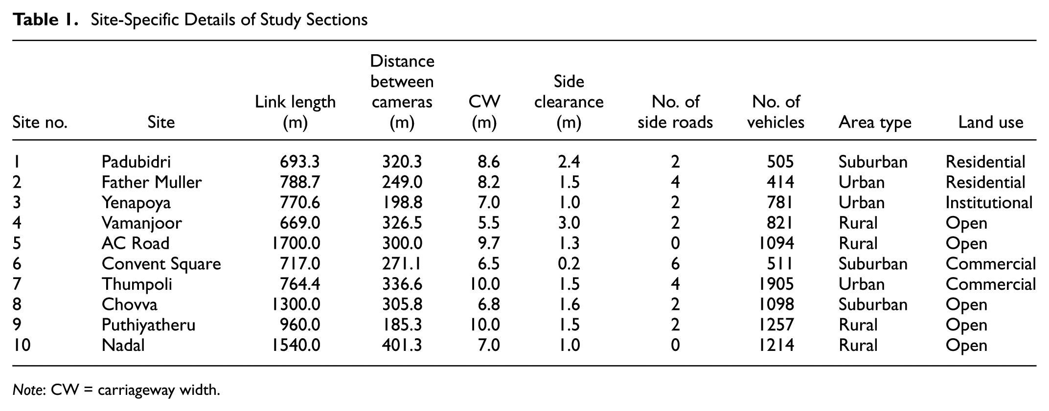
Note: CW = carriageway width.

Vehicle-specific details are extracted from the collected videos using spreadsheet and media player software. The travel times of vehicles for each site were estimated using vehicle re-identification technique. The difference in entry and exit times of a particular vehicle gives its free-flow travel time. From the known distance and travel time, FFS of each vehicle was estimated. Average FFS of vehicles in both directions is taken as the FFS since undivided roads are the subject of the study. The individual speeds are then aggregated into class-wise speeds and overall (all vehicle classes together) speeds for five-minute intervals. In the present study, vehicles are classified into six categories and the posted speed limits of each study site are shown in Table 2.

Table 2.

Details of Vehicle Classes and Subclasses Considered Including Speed Limits for Different Sites

Sl. no.	Class	Notation	Posted speed limits of sites (km/h)										Subclass
Sl. no.	Class	Notation	1	2	3	4	5	6	7	8	9	10	Subclass
1	Two-wheelers	TW	50	50	50	60	50	50	50	60	60	60	Motor bikes & Scooters
2	Three-wheelers	ThW	50	30	30	50	50	40	30	50	50	50	Passenger carriers & goods carriers
3	Passenger cars	Car	80	50	50	85	80	70	50	85	85	85	Hatchbacks, sedans & SUVs
4	Light commercial vehicles	LCV	65	50	50	65	65	60	50	65	65	65	Passenger carriers & goods carriers
5	Buses	Bus	65	40	40	65	65	60	40	65	65	65	Passenger carriers & institutional buses
6	Trucks	Truck	65	40	40	65	65	60	40	65	65	65	Trucks

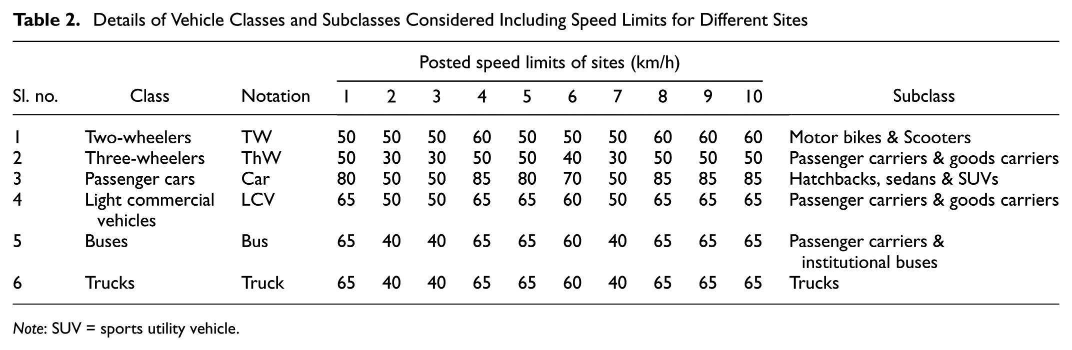
Note: SUV = sports utility vehicle.

Analysis of FFS

In this section, the details of vehicle composition in each site are given. The cumulative percentage of speeds based on vehicle-specific and site-specific characteristics are presented in this section. The influences of site-specific and vehicle-specific factors on FFS are also examined.

Vehicular Composition

In the present study, a total of 9,600 vehicles were analyzed, of which 34% were two-wheelers, 8% three-wheelers, 30% cars, and 7% light commercial vehicles, 7% buses, and 14% trucks. The majority of the vehicles were either two-wheelers or passenger cars. The proportion of light commercial vehicles and buses was found to be the minimum. Figure 1 shows the vehicle composition of the selected ten sections.

Figure 1.

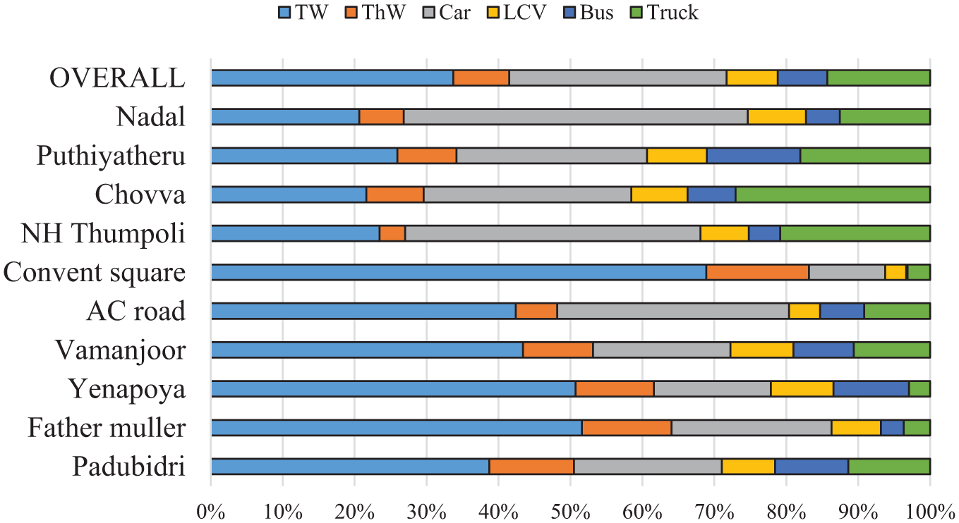
Stacked bar graph: vehicle composition in the selected study sections.

Cumulative Percentile Speed Curves

The 85th and 15th percentile speeds give a general description of the high and low speeds observed by most reasonable drivers. The 85th percentile speed is the speed that 85 percent of vehicles do not exceed. The speed limit is commonly set at or below the 85th percentile operating speed. The 50th percentile speed represents the average speed of the traffic stream. Figure 2 represents cumulative percentage frequency distribution curves for speeds of traffic stream (all vehicles together), different class of vehicles, area type, and land use types.

Figure 2.

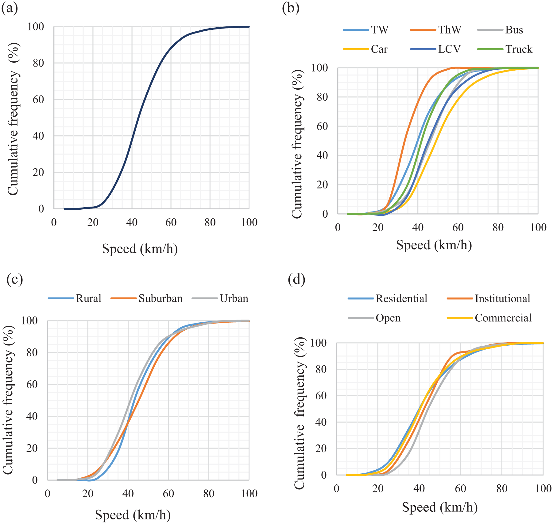
Cumulative percentile speed: (a) traffic stream; (b) class-wise; (c) area type; (d) land use.

The overall 85th percentile speed obtained is 58 km/h. The 50th percentile speed and 15th percentile speeds obtained are 43 km/h and 32 km/h, respectively. Cars have the highest 85th percentile speed (64 km/h) and three-wheelers have the lowest (43 km/h). Considering area types, suburban areas have higher 85th percentile speed (60 km/h) followed by rural (57 km/h) and urban (55 km/h) areas. The 50th percentile speed also follows the same trend as the 85th percentile speed but the 15th percentile speed is higher in rural areas (34 km/h). Open area land use type has higher 85th, 50th, and 15th percentile speeds. The 85th percentile speeds of institutional, commercial, residential, and open areas are 53 km/h, 55 km/h, 57 km/h, and 58 km/h, respectively. Similarly, the 15th percentile speeds are 28 km/h, 29 km/h, 31 km/h, and 4 km/h for residential, commercial, institutional, and open areas, respectively. The 50th percentile speed is highest in open areas (44 km/h) and lowest in residential areas (40 km/h).

Analysis of FFS for Different Vehicle Classes and Subclasses

The mean and the median FFS of vehicle classes and subclasses were almost equal, indicating normal distribution. Among vehicle classes, passenger cars (53.7 km/h) were found to be the fastest and three-wheelers (39.1 km/h) the slowest. Among subclasses considered in the study, the highest average speed was for sports utility vehicles (SUVs) (57.3 km/h) and the lowest for three-wheeler goods carriers (37.8 km/h). Considerable variation in standard deviation of speeds was also observed among vehicle groups.

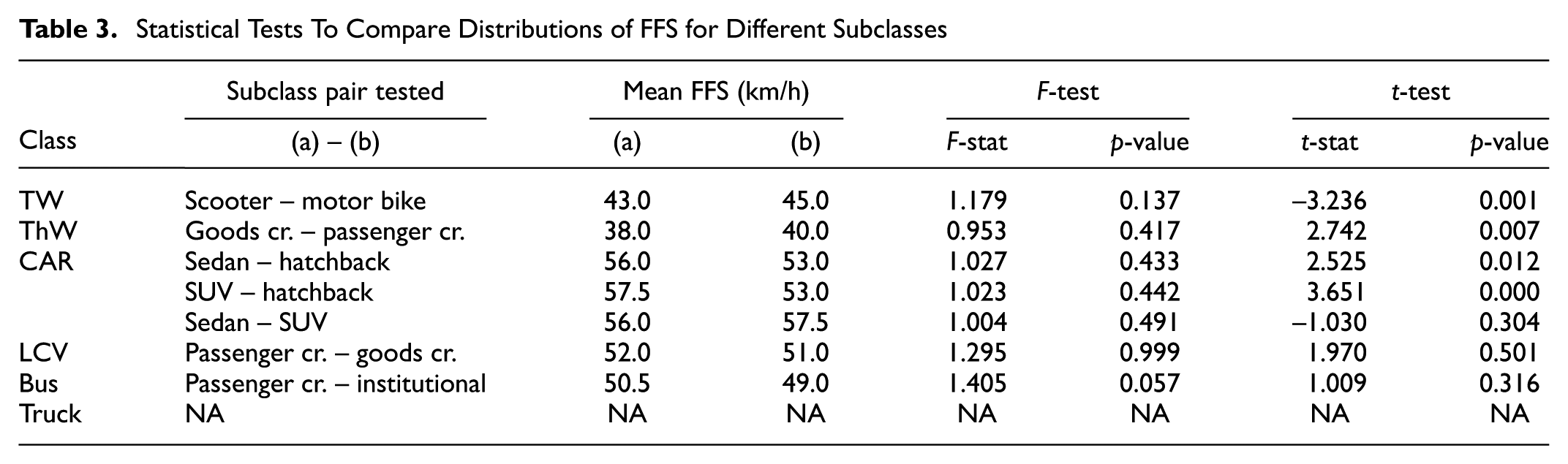
From Table 3 it is clear that, among two-wheelers, motorbikes and scooters had statistically different mean FFS. Within three-wheelers, passenger carriers had higher FFS than goods carriers. Among cars, the variance was found to be same for all subclasses. The FFS of SUVs was found to be the highest and that of hatchback the lowest. In light commercial vehicles, passenger carriers had higher FFS and variance than goods carriers. Among buses the FFS of both subclasses was found to be similar.

Table 3.

Statistical Tests To Compare Distributions of FFS for Different Subclasses

Class	Subclass pair tested	Mean FFS (km/h)		F-test		t-test
Class	(a) – (b)	(a)	(b)	F-stat	p-value	t-stat	p-value
TW	Scooter – motor bike	43.0	45.0	1.179	0.137	−3.236	0.001
ThW	Goods cr. – passenger cr.	38.0	40.0	0.953	0.417	2.742	0.007
CAR	Sedan – hatchback	56.0	53.0	1.027	0.433	2.525	0.012
	SUV – hatchback	57.5	53.0	1.023	0.442	3.651	0.000
	Sedan – SUV	56.0	57.5	1.004	0.491	−1.030	0.304
LCV	Passenger cr. – goods cr.	52.0	51.0	1.295	0.999	1.970	0.501
Bus	Passenger cr. – institutional	50.5	49.0	1.405	0.057	1.009	0.316
Truck	NA	NA	NA	NA	NA	NA	NA

Analysis of FFS for Different Area Type

Analysis was performed to understand the speed distributions of vehicle classes on urban, suburban, and rural roads. Of the ten study sections, three were chosen from urban areas, three from suburban areas, and four from rural areas. The overall and class-wise FFS variations are given in box plots in Figure 3a and 3c.

Figure 3.

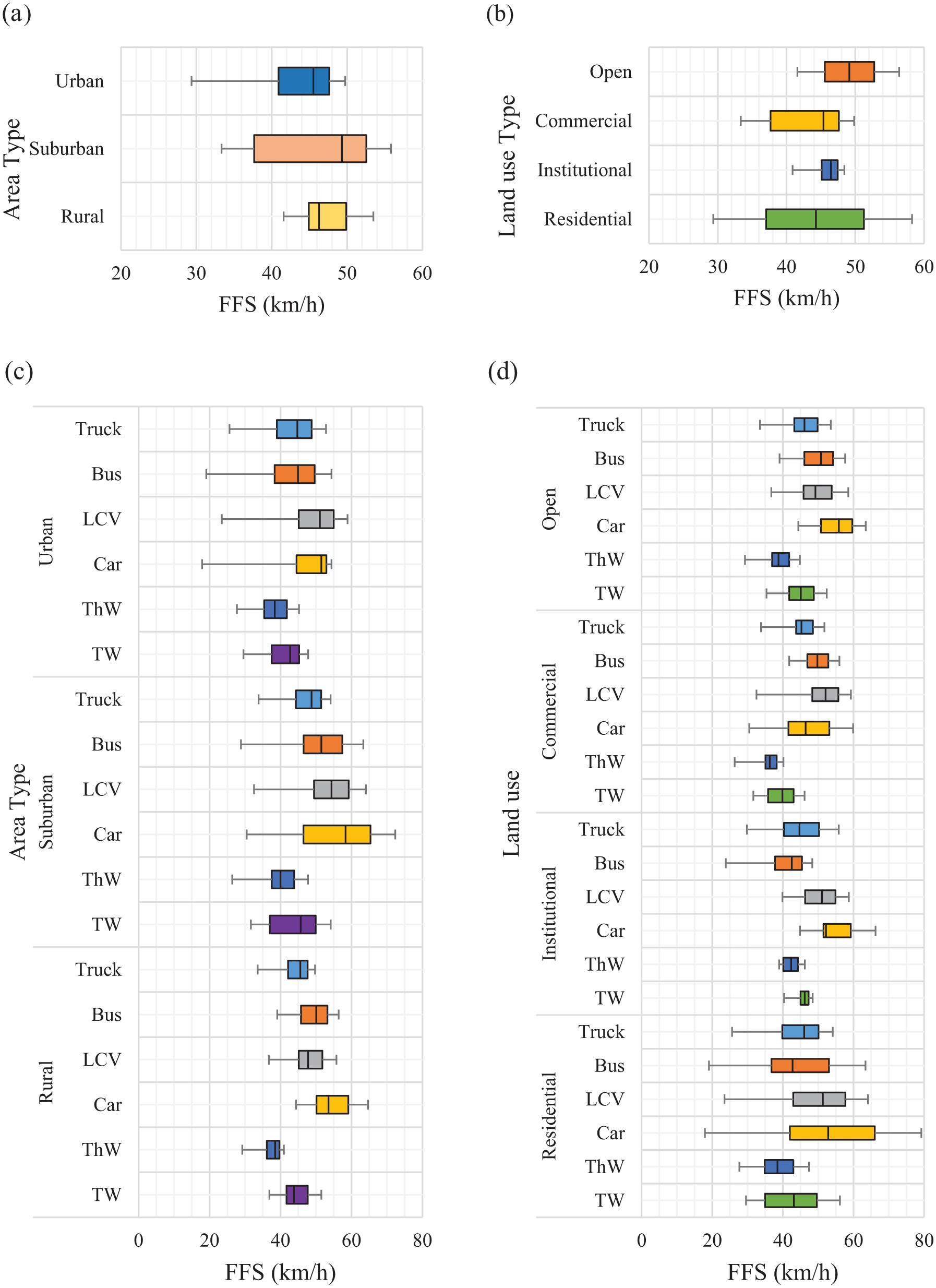
Box plots showing variation of FFS based on area type and land use type: (a) FFS on different area types; (b) FFS on different land use types; (c) class-wise FFS based on area type; (d) class-wise FFS based on land use type.

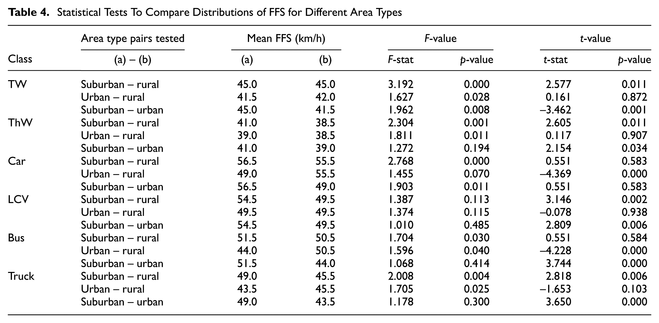
The mean overall FFS on rural roads, suburban roads, and urban roads was found to be 47.6 km/h, 46.4 km/h, and 43.4 km/h, respectively. On urban roads speeds are generally lower due to side friction. The statistical significance of the difference in means and variances of FFS on different area types were checked using F-tests and t-tests (Table 4). FFS is lowest for urban areas for all vehicle classes. Also, cars were found to have the highest FFS whereas three-wheelers have the lowest in all the area types.

Table 4.

Statistical Tests To Compare Distributions of FFS for Different Area Types

Class	Area type pairs tested	Mean FFS (km/h)		F-value		t-value
Class	(a) – (b)	(a)	(b)	F-stat	p-value	t-stat	p-value
TW	Suburban – rural	45.0	45.0	3.192	0.000	2.577	0.011
	Urban – rural	41.5	42.0	1.627	0.028	0.161	0.872
	Suburban – urban	45.0	41.5	1.962	0.008	−3.462	0.001
ThW	Suburban – rural	41.0	38.5	2.304	0.001	2.605	0.011
	Urban – rural	39.0	38.5	1.811	0.011	0.117	0.907
	Suburban – urban	41.0	39.0	1.272	0.194	2.154	0.034
Car	Suburban – rural	56.5	55.5	2.768	0.000	0.551	0.583
	Urban – rural	49.0	55.5	1.455	0.070	−4.369	0.000
	Suburban – urban	56.5	49.0	1.903	0.011	0.551	0.583
LCV	Suburban – rural	54.5	49.5	1.387	0.113	3.146	0.002
	Urban – rural	49.5	49.5	1.374	0.115	−0.078	0.938
	Suburban – urban	54.5	49.5	1.010	0.485	2.809	0.006
Bus	Suburban – rural	51.5	50.5	1.704	0.030	0.551	0.584
	Urban – rural	44.0	50.5	1.596	0.040	−4.228	0.000
	Suburban – urban	51.5	44.0	1.068	0.414	3.744	0.000
Truck	Suburban – rural	49.0	45.5	2.008	0.004	2.818	0.006
	Urban – rural	43.5	45.5	1.705	0.025	−1.653	0.103
	Suburban – urban	49.0	43.5	1.178	0.300	3.650	0.000

Analysis of FFS for Different Land Use Types

Land use represents the roadside activity and its intensity. FFS were grouped and analyzed based on various land use types. The highest overall FFS was observed in open areas, with a mean of 49.0 km/h, while the speed was lowest in commercial areas with a mean of 43.5 km/h. The mean FFS in institutional areas and residential areas was 46.1 km/h and 43.8 km/h, respectively. The overall and class-wise FFS variations are given in Figure 3b and d .

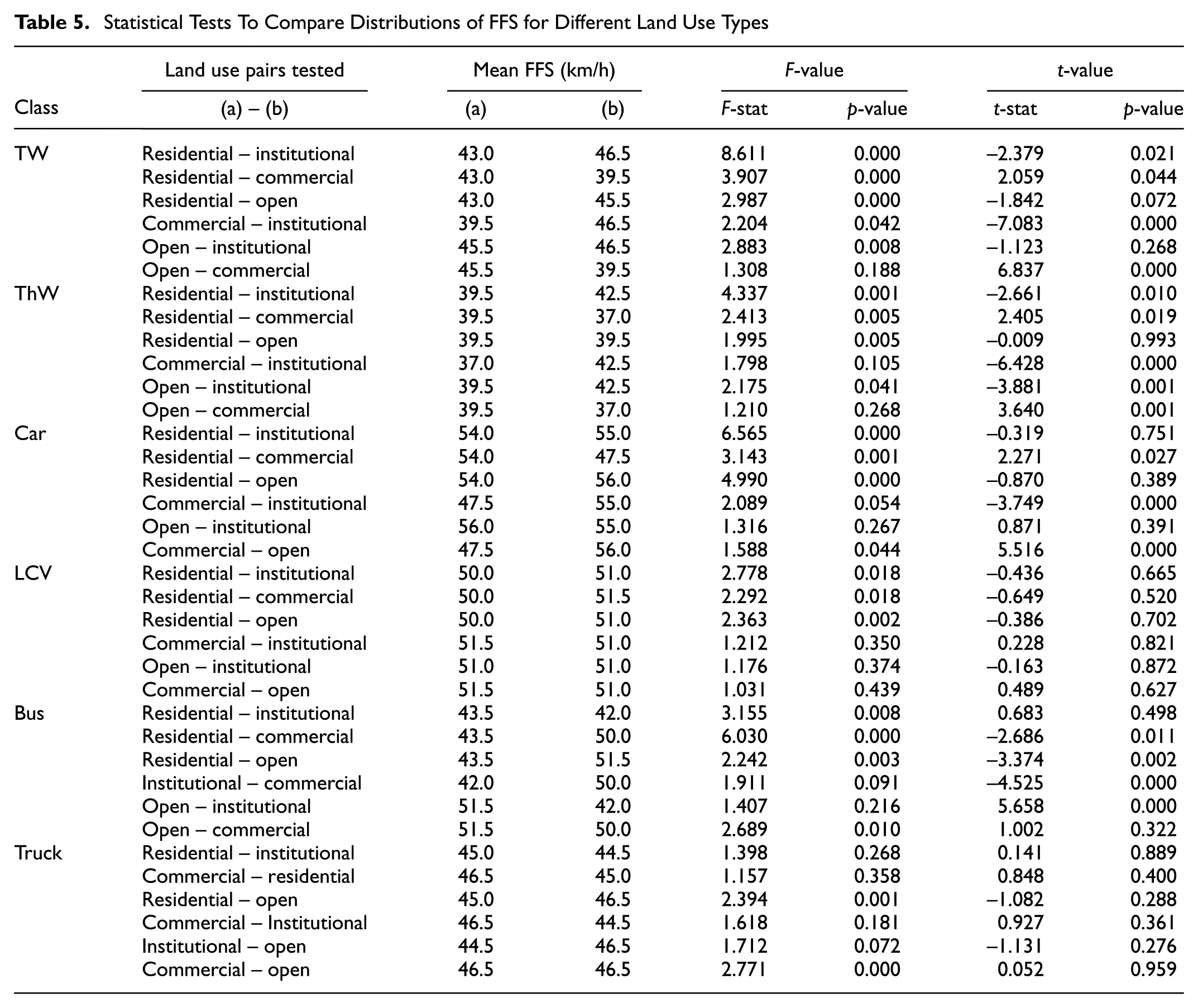
Statistical tests were conducted to understand the significance of difference in FFS across land use types for each vehicle class and the results are shown in Table 5. For all vehicle types, highest FFS was observed in open areas, followed by institutional areas, residential areas, and commercial areas. The reason for higher speed in open areas is the reduced side friction. Speeds in commercial and residential areas are lower due to buildings, more number of side roads, less lateral clearance, etc.

Table 5.

Statistical Tests To Compare Distributions of FFS for Different Land Use Types

Class	Land use pairs tested	Mean FFS (km/h)		F-value		t-value
Class	(a) – (b)	(a)	(b)	F-stat	p-value	t-stat	p-value
TW	Residential – institutional	43.0	46.5	8.611	0.000	−2.379	0.021
	Residential – commercial	43.0	39.5	3.907	0.000	2.059	0.044
	Residential – open	43.0	45.5	2.987	0.000	−1.842	0.072
	Commercial – institutional	39.5	46.5	2.204	0.042	−7.083	0.000
	Open – institutional	45.5	46.5	2.883	0.008	−1.123	0.268
	Open – commercial	45.5	39.5	1.308	0.188	6.837	0.000
ThW	Residential – institutional	39.5	42.5	4.337	0.001	−2.661	0.010
	Residential – commercial	39.5	37.0	2.413	0.005	2.405	0.019
	Residential – open	39.5	39.5	1.995	0.005	−0.009	0.993
	Commercial – institutional	37.0	42.5	1.798	0.105	−6.428	0.000
	Open – institutional	39.5	42.5	2.175	0.041	−3.881	0.001
	Open – commercial	39.5	37.0	1.210	0.268	3.640	0.001
Car	Residential – institutional	54.0	55.0	6.565	0.000	−0.319	0.751
	Residential – commercial	54.0	47.5	3.143	0.001	2.271	0.027
	Residential – open	54.0	56.0	4.990	0.000	−0.870	0.389
	Commercial – institutional	47.5	55.0	2.089	0.054	−3.749	0.000
	Open – institutional	56.0	55.0	1.316	0.267	0.871	0.391
	Commercial – open	47.5	56.0	1.588	0.044	5.516	0.000
LCV	Residential – institutional	50.0	51.0	2.778	0.018	−0.436	0.665
	Residential – commercial	50.0	51.5	2.292	0.018	−0.649	0.520
	Residential – open	50.0	51.0	2.363	0.002	−0.386	0.702
	Commercial – institutional	51.5	51.0	1.212	0.350	0.228	0.821
	Open – institutional	51.0	51.0	1.176	0.374	−0.163	0.872
	Commercial – open	51.5	51.0	1.031	0.439	0.489	0.627
Bus	Residential – institutional	43.5	42.0	3.155	0.008	0.683	0.498
	Residential – commercial	43.5	50.0	6.030	0.000	−2.686	0.011
	Residential – open	43.5	51.5	2.242	0.003	−3.374	0.002
	Institutional – commercial	42.0	50.0	1.911	0.091	−4.525	0.000
	Open – institutional	51.5	42.0	1.407	0.216	5.658	0.000
	Open – commercial	51.5	50.0	2.689	0.010	1.002	0.322
Truck	Residential – institutional	45.0	44.5	1.398	0.268	0.141	0.889
	Commercial – residential	46.5	45.0	1.157	0.358	0.848	0.400
	Residential – open	45.0	46.5	2.394	0.001	−1.082	0.288
	Commercial – Institutional	46.5	44.5	1.618	0.181	0.927	0.361
	Institutional – open	44.5	46.5	1.712	0.072	−1.131	0.276
	Commercial – open	46.5	46.5	2.771	0.000	0.052	0.959

Effect of Site-Specific Factors on FFS

The effect of quantitative variables on FFS was analyzed, and graphs with trend lines were plotted (Figure 4). The graphs show that FFS increases with increase in link length, carriageway width, and lateral clearance and decreases with increase in number of side roads.

Figure 4.

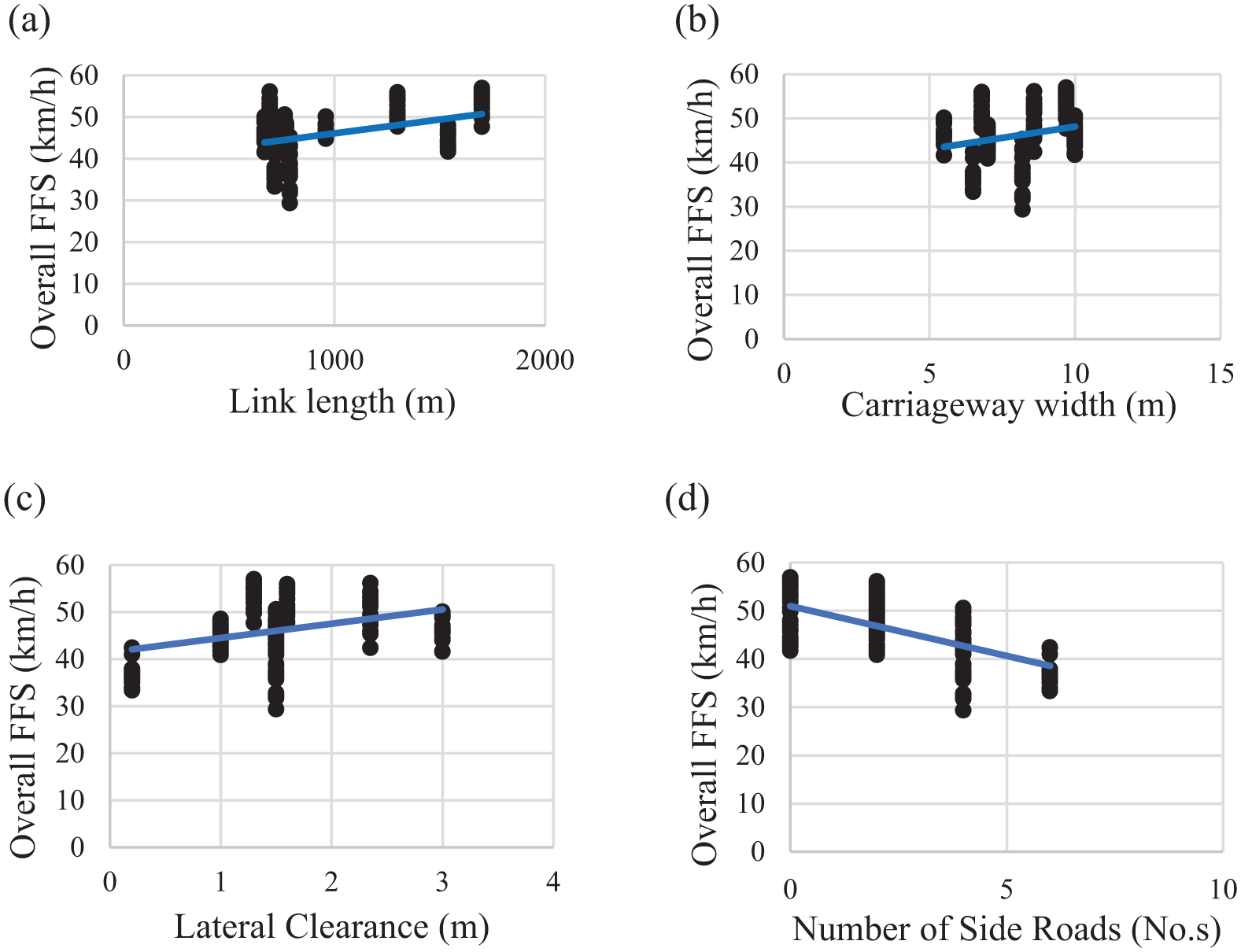
Effect of various site-specific factors on overall FFS: (a) link length; (b) carriageway width; (c) lateral clearance; (d) number of side roads.

Models for FFS

The FFS models were developed using regression analysis in SPSS software. Two sets of models were developed: general models and class-wise models. The general models were developed considering FFS of all vehicles classes together. The class-wise models include separate models for each of the six vehicle classes considered in the study. The foremost assumptions of regression analysis are that there must be no correlation among independent variables. Though this assumption is not perfectly attainable, minimizing the occurrence of correlated variables must be ensured in variable selection. Variable combinations are selected with the help of correlation matrix.

HCM Method of FFS Estimation

HCM 2010 ( 1 ) suggests the following equation to estimate FFS:

F F S = B F F S - f_{L S} - f_{A}

(1)

where FFS = estimated FFS (km/h); BFFS = base FFS (km/h); $f_{L S}$ = adjustment for lane and shoulder widths; $f_{A}$ = adjustment for access points.

The HCM method is valid only for homogeneous traffic and, in this study, other factors specific to Indian traffic conditions are also considered to develop FFS models.

General Model

FFS is selected as the dependent variable and total number of vehicles, heavy vehicle percentage, link length, carriageway width, lateral clearance, number of side roads, area type, and land use are selected as independent variables. Three models, GM1, GM2, GM3, are selected based on model goodness of fit, significance of model, and significance of independent variables (Table 6). The R² values of these models range from 0.299 to 0.771. Collinearity test, normality test, heteroskedasticity test, etc. are also done to verify the validity of the model. Among the general models, GM3 is recommended for having higher R² value (0.771).

Table 6.

General Models: Estimation of Coefficients, Goodness of Fit, and Significance

Model	R square	Variables	Coefficients	Std. error	t-value	Sig.
GM1	0.299	(Constant)	35.083	3.324	10.553	0.000
		No. of vehicles	−0.036	0.387	2.346	0.001
		Carriageway width	1.274	0.294	4.332	0.000
		Lateral clearance	1.683	0.531	3.169	0.002
		No. of side roads	−1.147	0.322	−3.567	0.001
GM2	0.503	(Constant)	32.228	2.773	11.621	0.000
		Carriageway width	1.334	0.297	4.491	0.000
		Lateral clearance	2.836	0.617	4.596	0.000
		Area suburban	−0.802	1.087	0.738	0.462
		Area urban	−3.423	1.070	−3.198	0.002
GM3	0.771	(Constant)	40.051	1.812	22.097	0.000
		No. of vehicles	−0.048	0.016	−3.029	0.003
		Carriageway width	2.004	0.240	8.354	0.000
		Lateral clearance	4.041	0.451	8.956	0.000
		No. of side roads	−2.595	0.195	−13.302	0.000
		Land use residential	−9.751	0.849	−11.485	0.000
		Land use institutional	−3.925	0.692	−5.676	0.000
		Land use commercial	−9.476	1.169	−8.106	0.000

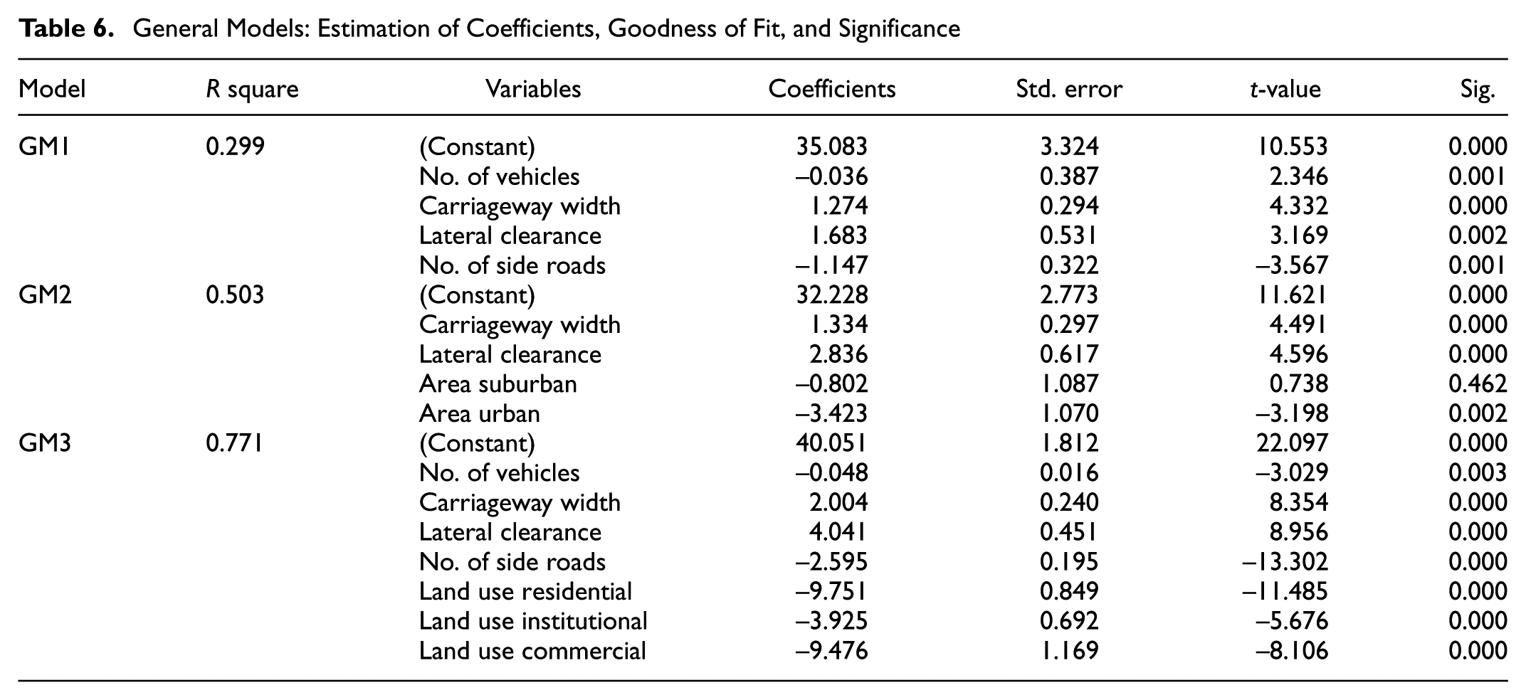
Model GM1 shows that FFS will be reduced by 0.036 km/h for an increase of one vehicle. For 1 m increase in carriage width and lateral clearance, FFS increases by 1.274 km/h and 1.683 km/h, respectively and increase in side roads decreases the speed by 1.147 km/h. Model GM2 predicts that for every 1 m increase in carriageway width, FFS increases by 1.334 km/h and for every 1 m increase in lateral clearance, speed increases by 2.836 km/h. FFS in suburban areas is 0.802 km/h lower than in rural areas. Moreover, in urban areas it is 3.423 km/h lower.

In model GM3, a 1 m increase in carriage width and lateral clearance increases FFS by 2.004 km/h and 4.041 km/h, respectively. Similarly, for one-unit increase in number of vehicles and number of side roads, FFS decreases by 0.048 km/h and 2.595 km/h, respectively. Also, FFS for land use types such as residential areas, institutional areas, and commercial areas are 9.751 km/h, 3.925 km/h and 9.476 km/h respectively, which are lower than for open area land use.

With reference to the model, carriageway width and lateral clearance have a positive effect on FFS. This is logical, as increase in carriageway width and lateral clearance enhances the smooth flow of traffic. Similarly, it can be inferred from the above model that the number of vehicles and number of side roads has a negative effect on FFS. That is, as the number of vehicles and number of side roads increases, it interrupts the free-flow of traffic.

Class-Wise Model

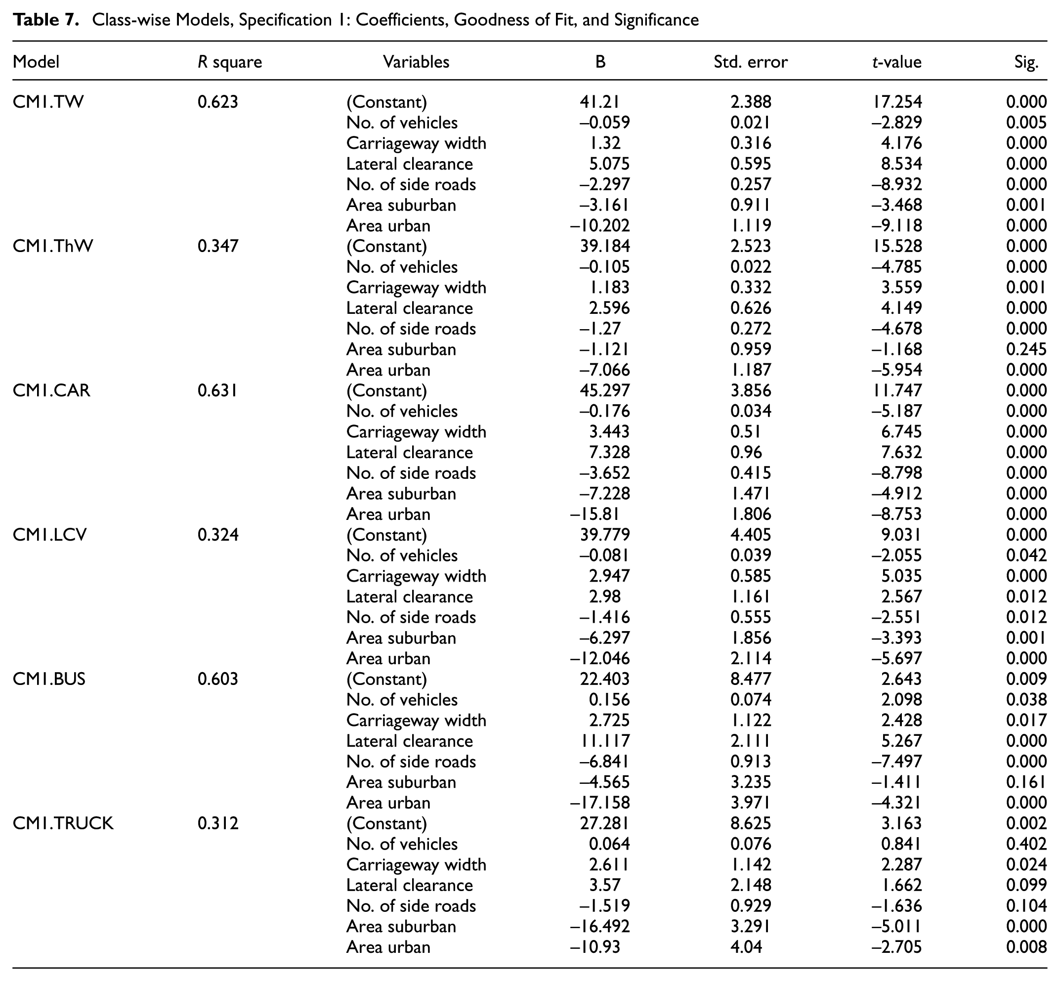
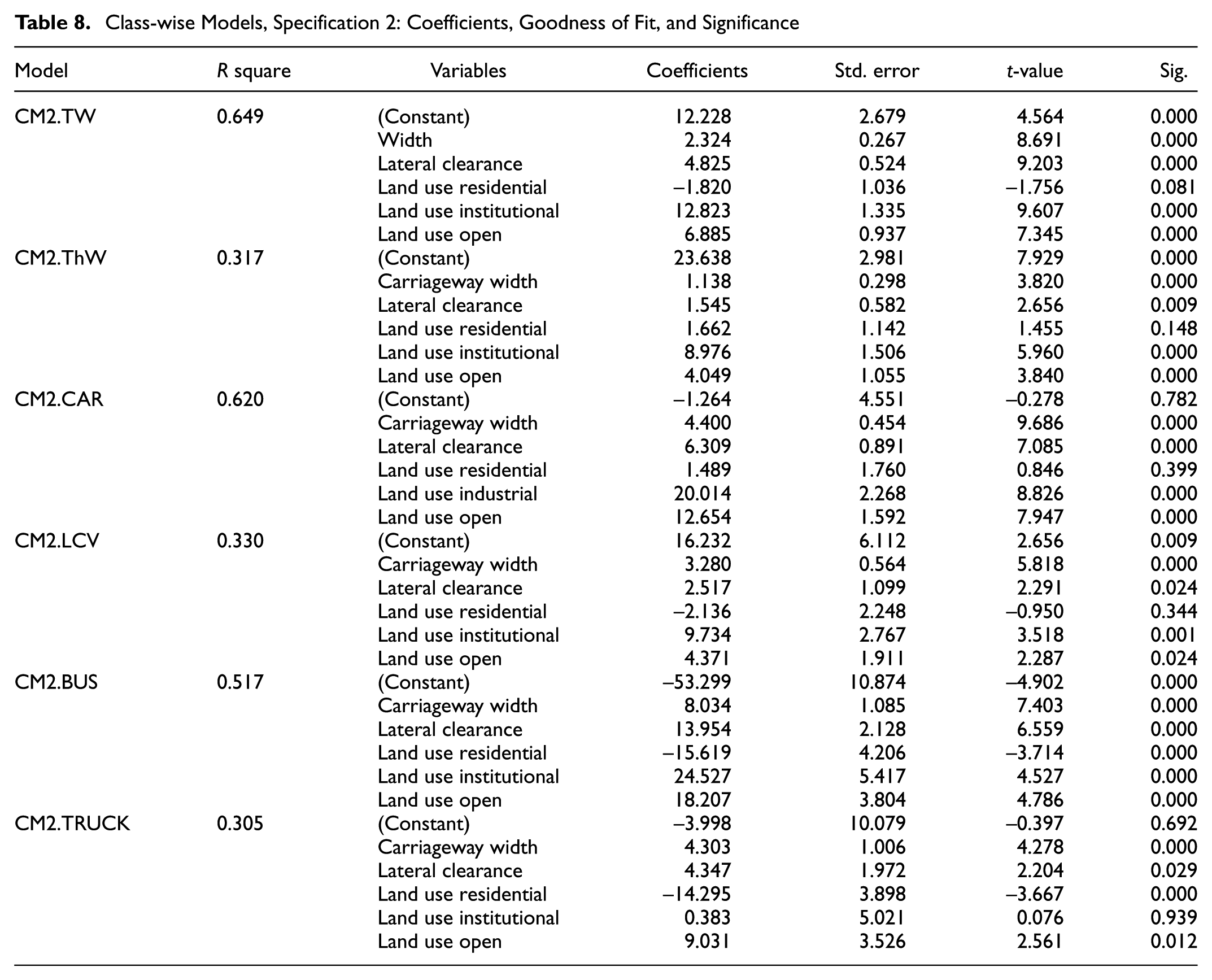
To study the effect of various factors on different vehicle classes, a class-wise regression model is developed for six classes of vehicles. Tables 7 and 8 show the goodness of fit, significance of model, and significance of independent variables for class-wise models of specifications 1 and 2.

Table 7.

Class-wise Models, Specification 1: Coefficients, Goodness of Fit, and Significance

Model	R square	Variables	B	Std. error	t-value	Sig.
CM1.TW	0.623	(Constant)	41.21	2.388	17.254	0.000
		No. of vehicles	−0.059	0.021	−2.829	0.005
		Carriageway width	1.32	0.316	4.176	0.000
		Lateral clearance	5.075	0.595	8.534	0.000
		No. of side roads	−2.297	0.257	−8.932	0.000
		Area suburban	−3.161	0.911	−3.468	0.001
		Area urban	−10.202	1.119	−9.118	0.000
CM1.ThW	0.347	(Constant)	39.184	2.523	15.528	0.000
		No. of vehicles	−0.105	0.022	−4.785	0.000
		Carriageway width	1.183	0.332	3.559	0.001
		Lateral clearance	2.596	0.626	4.149	0.000
		No. of side roads	−1.27	0.272	−4.678	0.000
		Area suburban	−1.121	0.959	−1.168	0.245
		Area urban	−7.066	1.187	−5.954	0.000
CM1.CAR	0.631	(Constant)	45.297	3.856	11.747	0.000
		No. of vehicles	−0.176	0.034	−5.187	0.000
		Carriageway width	3.443	0.51	6.745	0.000
		Lateral clearance	7.328	0.96	7.632	0.000
		No. of side roads	−3.652	0.415	−8.798	0.000
		Area suburban	−7.228	1.471	−4.912	0.000
		Area urban	−15.81	1.806	−8.753	0.000
CM1.LCV	0.324	(Constant)	39.779	4.405	9.031	0.000
		No. of vehicles	−0.081	0.039	−2.055	0.042
		Carriageway width	2.947	0.585	5.035	0.000
		Lateral clearance	2.98	1.161	2.567	0.012
		No. of side roads	−1.416	0.555	−2.551	0.012
		Area suburban	−6.297	1.856	−3.393	0.001
		Area urban	−12.046	2.114	−5.697	0.000
CM1.BUS	0.603	(Constant)	22.403	8.477	2.643	0.009
		No. of vehicles	0.156	0.074	2.098	0.038
		Carriageway width	2.725	1.122	2.428	0.017
		Lateral clearance	11.117	2.111	5.267	0.000
		No. of side roads	−6.841	0.913	−7.497	0.000
		Area suburban	−4.565	3.235	−1.411	0.161
		Area urban	−17.158	3.971	−4.321	0.000
CM1.TRUCK	0.312	(Constant)	27.281	8.625	3.163	0.002
		No. of vehicles	0.064	0.076	0.841	0.402
		Carriageway width	2.611	1.142	2.287	0.024
		Lateral clearance	3.57	2.148	1.662	0.099
		No. of side roads	−1.519	0.929	−1.636	0.104
		Area suburban	−16.492	3.291	−5.011	0.000
		Area urban	−10.93	4.04	−2.705	0.008

Table 8.

Class-wise Models, Specification 2: Coefficients, Goodness of Fit, and Significance

Model	R square	Variables	Coefficients	Std. error	t-value	Sig.
CM2.TW	0.649	(Constant)	12.228	2.679	4.564	0.000
		Width	2.324	0.267	8.691	0.000
		Lateral clearance	4.825	0.524	9.203	0.000
		Land use residential	−1.820	1.036	−1.756	0.081
		Land use institutional	12.823	1.335	9.607	0.000
		Land use open	6.885	0.937	7.345	0.000
CM2.ThW	0.317	(Constant)	23.638	2.981	7.929	0.000
		Carriageway width	1.138	0.298	3.820	0.000
		Lateral clearance	1.545	0.582	2.656	0.009
		Land use residential	1.662	1.142	1.455	0.148
		Land use institutional	8.976	1.506	5.960	0.000
		Land use open	4.049	1.055	3.840	0.000
CM2.CAR	0.620	(Constant)	−1.264	4.551	−0.278	0.782
		Carriageway width	4.400	0.454	9.686	0.000
		Lateral clearance	6.309	0.891	7.085	0.000
		Land use residential	1.489	1.760	0.846	0.399
		Land use industrial	20.014	2.268	8.826	0.000
		Land use open	12.654	1.592	7.947	0.000
CM2.LCV	0.330	(Constant)	16.232	6.112	2.656	0.009
		Carriageway width	3.280	0.564	5.818	0.000
		Lateral clearance	2.517	1.099	2.291	0.024
		Land use residential	−2.136	2.248	−0.950	0.344
		Land use institutional	9.734	2.767	3.518	0.001
		Land use open	4.371	1.911	2.287	0.024
CM2.BUS	0.517	(Constant)	−53.299	10.874	−4.902	0.000
		Carriageway width	8.034	1.085	7.403	0.000
		Lateral clearance	13.954	2.128	6.559	0.000
		Land use residential	−15.619	4.206	−3.714	0.000
		Land use institutional	24.527	5.417	4.527	0.000
		Land use open	18.207	3.804	4.786	0.000
CM2.TRUCK	0.305	(Constant)	−3.998	10.079	−0.397	0.692
		Carriageway width	4.303	1.006	4.278	0.000
		Lateral clearance	4.347	1.972	2.204	0.029
		Land use residential	−14.295	3.898	−3.667	0.000
		Land use institutional	0.383	5.021	0.076	0.939
		Land use open	9.031	3.526	2.561	0.012

FFS from specification 1 model can be obtained using Equation 1.

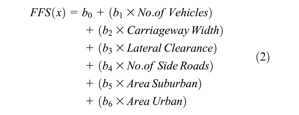
\begin{matrix} F F S (x) = b_{0} + (b_{1} \times N o . o f V e h i c l e s) \\ + (b_{2} \times C a r r i a g e w a y W i d t h) \\ + (b_{3} \times L a t e r a l C l e a r a n c e) \\ + (b_{4} \times N o . o f S i d e R o a d s) \\ + (b_{5} \times A r e a S u b u r b a n) \\ + (b_{6} \times A r e a U r b a n) \end{matrix}

(2)

Similarly, FFS from specification 2 model is obtained using Equation 2.

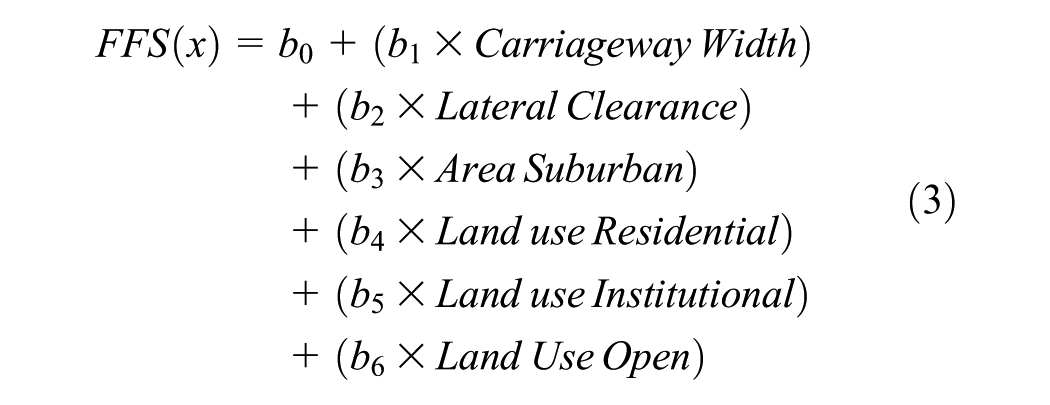
\begin{matrix} F F S (x) = b_{0} + (b_{1} \times C a r r i a g e w a y W i d t h) \\ + (b_{2} \times L a t e r a l C l e a r a n c e) \\ + (b_{3} \times A r e a S u b u r b a n) \\ + (b_{4} \times L a n d u s e R e s i d e n t i a l) \\ + (b_{5} \times L a n d u s e I n s t i t u t i o n a l) \\ + (b_{6} \times L a n d U s e O p e n) \end{matrix}

(3)

where x is the class of vehicle.

R² values of these models range from 0.305 to 0.649. CM2.TW model is recommended based on higher R² value (0.649). It can be concluded from all the models that both carriageway width and lateral clearance have a positive effect on FFS. That is, as carriageway width and lateral clearance increases, FFS also increases. From specification 1, it is seen that FFS decreases with increase in number of vehicles in the traffic stream, except for heavy vehicles (buses and trucks). Also, it was found that as the number of side roads increases FFS decreases. The speed of vehicles in urban and suburban areas is found to be lower than in rural areas. It is also seen that for different land use types, different vehicles have different trends in FFS.

Prediction of Overall FFS using Class-Wise Models

In the present study, class-wise models are used to estimate the FFS of six classes of vehicles. These models can be employed to obtain the overall FFS, as shown in Equation 3.

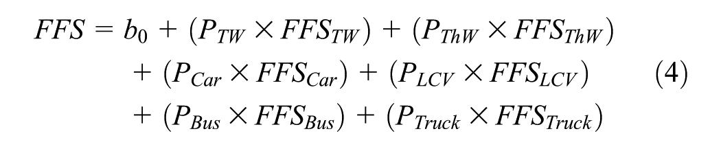
\begin{matrix} F F S = b_{0} + (P_{T W} \times F F S_{T W}) + (P_{T h W} \times F F S_{T h W}) \\ + (P_{C a r} \times F F S_{C a r}) + (P_{L C V} \times F F S_{L C V}) \\ + (P_{B u s} \times F F S_{B u s}) + (P_{T r u c k} \times F F S_{T r u c k}) \end{matrix}

(4)

where

FFS is the overall FFS;

$F F S_{T W}$ , $F F S_{T h W}$ , …………. $, F F S_{T r u c k}$ are the class-wise FFS in the study stretch

$P_{T W}$ , $P_{T h W},$ …………., $P_{T r u c k}$ are the class-wise proportions.

Validation of Models

In the validation stage, an attempt was made to understand how well the models could predict the outcome of an independent sample from the same population. The FFS prediction models were built using 72.2% of data collected. The models were internally validated using the same 72.2% data (internal validation) and externally validated using the remaining 27.8% data (external validation). The data for model development and validation were selected randomly from the whole sample. The predicted values of FFS were compared with the observed FFS and mean absolute percentage error (MAPE) was computed. MAPE values of general and class-wise models are found to vary between 7% and 25%. MAPE values of all general and class-wise models, except class-wise model for buses and trucks, are found to vary between 7% and 20% which shows that the models are reasonably successful at predicting FFS.

Summary and Conclusions

The present study aims to develop models for predicting free-flow speed (FFS) on undivided roads, which are common road facilities in India. The study evolved the variability in FFS among different vehicle classes which are considered to be an important aspect in mixed traffic conditions. Data were collected from ten different sites having different site-specific characteristics located in southern parts of India using videographic technique. Variations of FFS with site-specific and vehicle-specific factors were checked using statistical tests and FFS prediction models were developed. General (all vehicles together) and class-wise models were developed using SPSS software. The key conclusions arising from the study are:

The overall 85th percentile speed, 50th percentile speed and 15th percentile speed of vehicles considering all sites are 58 km/h 43 km/h and 32 km/h, respectively.

Cars have highest 85th percentile speed (64 km/h) and three-wheelers have the lowest (43 km/h). While considering area type, suburban have higher 85th percentile speed (60 km/h) and urban has the lowest (55 km/h). Open area land use type has the highest 85th percentile speed (58 km/h) followed by residential areas (57 km/h).

FFS of six vehicle classes under study vary significantly. The increasing order of FFS among the vehicle classes is as follows: three-wheelers (39.1 km/h), two-wheelers (43.7 km/h), trucks (46.0 km/h), buses (48.6 km/h), light commercial vehicles (50.7 km/h) and cars (53.6 km/h).

Mean overall FFS in rural areas (47.6 km/h) is higher than suburban (46.4 km/h) and urban areas (43.4 km/h). On urban roads speeds are generally lesser due to side friction.

Mean overall FFS in open areas (48.9 km/h) is higher than residential, institutional, and commercial areas. The reason for higher speeds in open areas is due to reduced side friction in open areas. FFS in commercial and residential areas is lower due to buildings, more number of side roads, lesser lateral clearance, etc.

From all the models and statistical tests, it is clear that carriageway width, lateral clearance, and link length have a positive effect on FFS.

From general models, it can be inferred that number of vehicles and number of side roads adversely affects FFS.

Class-wise models show that the influence of site factors on FFS varies significantly across vehicle classes.

The developed models can be used for planning and operational analysis of undivided roads. The findings will be helpful to traffic planners and engineers for regulation and control of traffic operations, geometric design of roads, accident analysis, before-and-after studies of road improvement schemes, assessing journey times, and congestion on roads and in correlating capacity with speeds.

The study findings can be generalized by collecting data from various sites and also, by selecting additional independent variables (e.g., driver behavior, vehicular condition, environmental factors, road geometry, functional properties of the road, etc.). The same methodology can be adopted for developing models for other types of roads (e.g., divided roads, multilane highways, etc.).

Footnotes

Author Contributions

The authors confirm contribution to the paper as follows: study conception and design: Gowri Asaithambi and Vipin; data collection: Vipin; analysis and interpretation of results: Gowri Asaithambi and Vipin; draft manuscript preparation: Vipin and Gowri Asaithambi. All authors reviewed the results and approved the final version of the manuscript.

The Standing Committee on Highway Capacity and Quality of Service (AHB40) peer-reviewed this paper (18-01831).

References

Highway Capacity Manual 2010 . Transportation Research Board of the National Academies, Washington, D.C., 2010.

Bang

K. L.

Impact of Side Friction on Speed-Flow Relationships for Rural and Urban Highways. Technical Report. SWEROAD Indonesia, Bandung, Indonesia, 1995.

Dixon

K. K.

C. H.

Sarasua

Daniel

Posted and Free-flow Speeds for Rural Multilane Highways in Georgia. Journal of Transportation Engineering, Vol. 125, No. 6, 1999, pp. 487–494.

Tarko

Sinha

K. C.

Model of Free-Flow Speed for Indiana Arterial Roads. Transportation Research Record: Journal of the Transportation Research Board, 2001. 1776: 189–193.

Kyte

Khatib

Shannon

Kitchener

Effect of Environmental Factors on Free-Flow Speed. Transportation Research Circular E-C018, 2005, pp. 108–119.

Hablas

H. E.

A Study of Inclement Weather Impacts on Freeway Free-Flow Speed. Technical Report. Civil and Environmental Engineering, Virginia Polytechnic Institute and State University, Blacksburg, Virginia, 2007.

Wang

L. X.

The Study of Establishing Realistic Road Speed Limits. Research Journal of Applied Sciences Engineering and Technology, Vol. 4, No. 6, 2012, pp. 599–602.

Hashim

I. H.

Analysis of Speed Characteristics for Rural Two-lane Roads: A Field Study from Minoufiya Governorate, Egypt. Ain Shams Engineering Journal, 2011, pp. 43–52.

Azai

T. A.

Vien

L. L.

Factors Affecting Free-Flow Speed at Multilane Highways in Malaysia. Caspian Journal of Applied Sciences Research, Vol. 2(AICCE’12 & GIZ’ 12), 2013, pp. 28–35.

10.

Moses

Mtoi

Evaluation of Free Flow Speeds on Interrupted Flow Facilities. Technical Report. Department of Civil Engineering, FAMU-FSU College of Engineering, Tallahassee, Fla., 2013.

11.

Wang

Harvey

Lea

J. D.

Kim

Impact of Pavement Roughness on Vehicle Free-Flow Speed. Technical Memorandum, California Department of Transportation Division of Research, Innovation and System Information, 2013.

12.

Andrade

G. R.

Pitombo

C. S.

Cunha

A. L.

Setti

J. R.

A Model for Estimating Free-Flow Speed on Brazilian Expressways. Transportation Research Procedia, Vol. 15, 2016, pp. 378–388.

13.

Zeng

Yang

(2010). Impact of Lane Width on Vehicle Speed of Urban Arterials. In ICCTP: Integrated Transportation Systems: Green, Intelligent, Reliable. American Society of Civil Engineers, Beijing, China, 2010, pp. 1844–1852.

14.

Tunde

I. Y.

The Factors for Free Flow Speed on Urban Arterials – Empirical Evidences from Nigeria. Journal of American Science, Vol. 6, No. 12, 2010, pp. 1487–1497.

15.

Tseng

P. Y.

Lin

F. B.

Chang

C. W.

Analysis of Free-flow Speed Characteristics of Urban Arterials. Asian Transport Studies, Vol. 2, No. 4, 2013, pp. 363–378.

16.

Puan

O. C.

Abdurrahman

U. T.

Application of Moving Car Observer Method for Measuring Free Flow Speed on Two-lane Highways. Jurnal Teknologi, Vol. 69, No. 2, 2014, pp. 15–19.

17.

Balakrishnan

Sivanandan

Influence of lane and vehicle subclass on free-flow speeds for urban roads in heterogeneous traffic. Transportation Research Procedia, Vol. 10, 2015, pp. 166–175.

18.

Rao

A. M.

Rao

K. R.

Free Speed Modeling for Urban Arterials - A Case Study on Delhi. Periodica Polytechnica Transportation Engineering, Vol. 43, No. 3, 2015, pp. 111–119.

19.

Yusuf

I. T.

Adeleke

O. O.

Salami

A. W.

Ayanshola

A. M.

The Factors that Affect the Free Flow Speed on an Arterial in Ilorin, Nigeria. Nigerian Journal of Technology, Vol. 35, No. 3, 2016, pp. 473–480.