
Abstract
Performance measures are essential for managing transportation systems, including signalized corridors. Coordination is an essential element of signal timing, enabling reliable progression of traffic along corridors. Improved progression leads to less user delay, which leads to user cost savings and lower vehicle emissions. This paper presents a comparative study of signal coordination assessment using four different technologies. These technologies include detector-based high-resolution controller data, Bluetooth/Wi-Fi sensors, segment-based probe vehicle data, and automated vehicle location data consisting of GPS-based vehicle trajectories, representing the data anticipated from emerging connected vehicle technologies. The data were compiled for a 4.2-mi corridor in Holland, Michigan. The results show that all of the data sources were able to identify, at some level, where coordination issues existed. Detector-based controller data and GPS-based vehicle trajectory data were capable of showing greater detail, and could be used to make offset adjustments. The paper concludes by demonstrating the identification of signal coordination issues with the use of visual performance metrics incorporating automated vehicle location (AVL) trajectory data.
Coordination is an essential aspect of signal operation. One basic way to evaluate the quality of progression is to measure the travel time of vehicles along the corridor. Historically, this has been done with floating car studies. GPS instruments increased the fidelity of floating car studies ( 1 ), but data collection remained labor intensive. Automatic vehicle identification (AVI) methods ( 2 – 5 ), such as using Bluetooth/Wi-Fi technologies, have greatly increased the sample sizes in travel time studies, but require additional infrastructure and do not provide the trajectory data.
With the advent of ubiquitous mobile GPS devices such as smartphones and commercial navigation devices, opportunities to obtain automated vehicle location (AVL) data at low cost have emerged. Initial data products using this strategy were timestamped average segment speeds, which have been applied to arterials ( 6 – 8 ). The advantage of this type of data is that no infrastructure is needed, but aggregation to 1-min or longer intervals loses a considerable amount of operational detail present in the vehicle trajectories. Statistical comparisons of the AVI and AVL data sets show a comparable accuracy for speed assessment over time ( 9 , 10 ).
Recently, AVL data has been explored for such purposes, either in anticipation of dedicated short range communications–based (DSRC) connected vehicle data in future, or using crowdsourced vehicle trajectories from commercial data providers. A critical issue with AVL data is the penetration rate of the vehicle fleet; at present, very few vehicles are equipped with the onboard units necessary to communicate with roadside infrastructure, which is itself nascent. Previous studies on use of AVL data have mainly focused on opportunities to improve signal control by integration of AVL data into the control system ( 11 – 14 ). Such methods have required relatively high penetration rates of perhaps 25% or more, which is much higher than present rates. A few studies have focused on performance evaluation, for which much lower penetration rates can provide useful results, as has been shown in previous studies ( 15 – 19 ). It is possible to compensate for low penetration rates by extending the sample period; this is possible by aligning similar time-of-day and day-of-week patterns. This paper examines potential uses of AVL data to evaluate signal coordination by aggregating trajectory data for similar time periods to build a large enough sample of data to determine characteristics of vehicle coordination.
The paper uses a signalized corridor in Holland, Michigan to investigate four different approaches for identifying and characterizing coordination issues. Bluetooth/Wi-Fi media access control (MAC) address devices, segment-based probe vehicle data, detector-based signal performance measures, and AVL trajectory data are used to evaluate the same corridor. The paper summarizes the strengths and weaknesses of each of the technologies and provides a perspective on the future of AVL trajectory data.
Performance Measurement with AVL Data
A few previous studies have examined the use of AVL data for the purpose of developing signal performance measures. Argote-Cabañero et al. considered an application for estimating Highway Capacity Manual metrics for 15-min analysis periods ( 15 ). They suggested that a penetration rate of 15% would likely be needed for accurate results for that time frame.
In a proof of concept study for measuring cyclic arrival patterns, Day and Bullock examined the ability of such patterns to feed an offset optimization process at very low penetration rates, considering sample periods of 3 h or 15 min ( 16 ). For these applications, the results suggested that penetration rates of 5% would work for 15 min and 1% would work for 3 h (e.g., for generating cyclic flow profiles for a time-of-day plan). Layering data from multiple days could potentially lower the penetration rate to 0.1%. This study was followed up with a field study using AVL data from a private sector provider. With penetration rates varying between approximately 0.1% and 0.5%, and data aggregated over a 6-week period, cyclic flow profiles were generated and used for offset optimization; they performed as well as optimal offsets generated from detector data on the same corridors.
A study by Wünsch et al. used AVL data to estimate movement delays at signalized intersections in Bavaria ( 18 ). This study applied a geofencing technique to identify zones of influence around intersections, and an automated process to determine the paths of vehicular movements at 2,300 intersections. This work was accomplished using the available penetration rates of navigation devices at the time of the study.
Zheng and Liu developed a method for estimating movement volumes using AVL data at low penetration rates ( 19 ). This method included aggregating AVL data over numerous days. The method was applied on corridors in the Ann Arbor, Michigan connected vehicle testbed and with commercial data in China. The method was found to estimate volumes with mean absolute percentage errors of 9% to 12%.
US-31 Corridor in Holland, Michigan
The US-31 corridor in Holland, Michigan is a 4.2-mi north–south corridor with an annual average daily traffic (AADT) of between 30,000 and 40,000 vehicles (see Figure 1). The corridor currently operates in fixed time with seven signals in the southbound (SB) direction and six signals in the northbound (NB) direction. As the corridor was recently reconstructed, it consistently operates below capacity. The corridor is located just east of Holland, which is a 30,000-resident town on Michigan’s western lake shore. The Michigan Department of Transportation is currently installing and testing a detector-based signal performance measure system on this corridor; however, no adjustments have been made on the corridor’s signal timings throughout this data collection procedure. As part of this project, data is being collected to determine the baseline travel behavior on this corridor. The data being collected includes Bluetooth/Wi-Fi probe vehicle data, crowdsourced GPS probe vehicle data, and detector and phasing events from the signal controller. In addition, 2 weeks of AVL trajectory data were provided for comparison by INRIX.
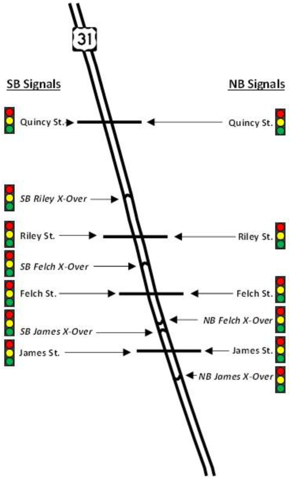
US-31 corridor in Holland, Michigan.
Methodology
Four technologies were assessed for corridor performance measurement. It was desired to use the data to determine whether coordination issues exist and identify necessary adjustments. The four technologies are explained in depth below.
Signal Performance Measures
Detector-based signal performance measures based on high-resolution data are becoming a standard tool for determining performance of a signalized corridor. The Purdue Coordination Diagram, or PCD, allows the visualization of arrivals on green using phase and detector data from the signal controller. This visualization was constructed for each signalized intersection of the Holland corridor for a single day (Wednesday, July 12th, 2017). The corridor has various coordination issues as highlighted below.
Observations for NB US-31:
Figure 2i—Random arrivals at the South James crossover;
Figure 2ii—Poor offset during the 05:00–09:00 timing plan at James Street;
Figure 2iii—Early arrivals at the South Felch crossover during the 05:00–09:00 timing plan;
Figure 2iv—Late arrivals at the South Felch crossover in the 14:00–21:00 timing plan;
Figure 2v—Late arrivals at the Felch intersection in the 14:00–21:00 timing plan;
Figure 2vi—Platoon clipping at Riley Street; and
Figure 2vii—Heavy platoon dispersion on the approach to Quincy Street.
Observations for SB US-31:
Figure 2viii—Random arrivals at the Quincy intersection;
Figure 2ix—Numerous turning vehicles from Riley arriving on red; and
Figure 2x—Slightly early arrivals in the 14:00–21:00 timing plan at James Street.
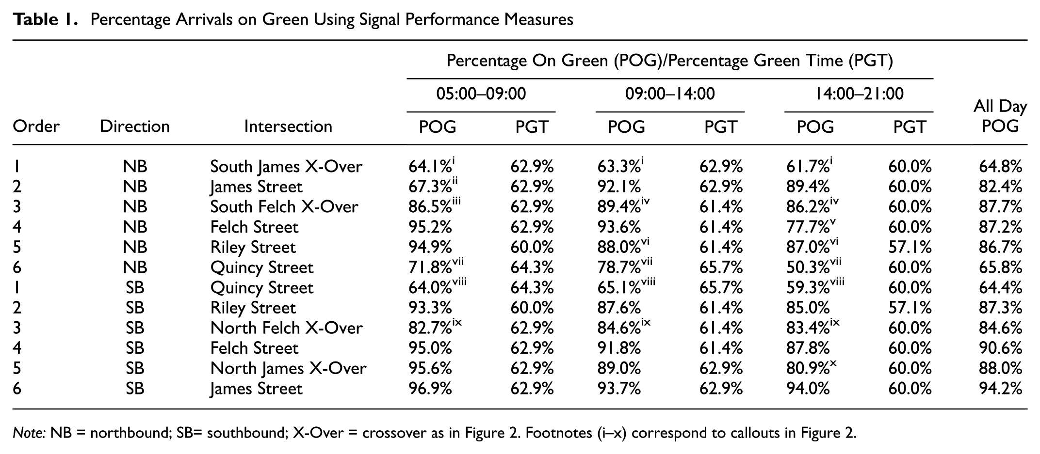
These graphics suggest that the SB direction is better coordinated during all of the timing plans throughout the day. The percentages of arrivals on green were calculated for each of the intersections in each direction. The callouts in Figure 2 are placed in Table 1 at the corresponding approach and time-of-day. Over the entire day, a majority of the intersections seem to be performing well. The worst performing non-random arrival approach is NB at Quincy, with arrivals of 65.8% over the course of the day. These issues identified by the detector data will help determine the ability of other data sets to also identify such issues.
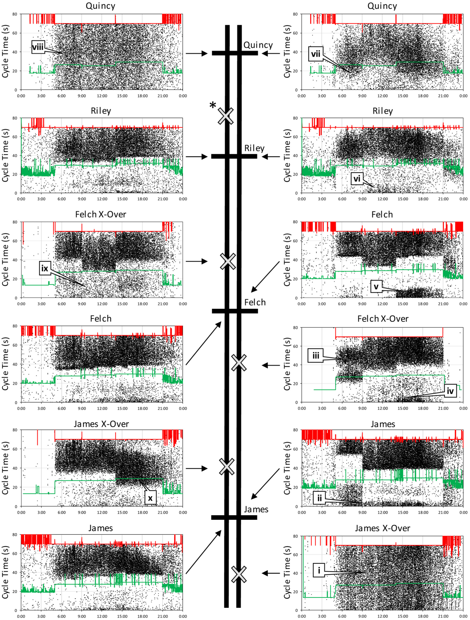
Purdue Coordination Diagrams for the US-31 Holland corridor (7/12/2017). The North Riley crossover (marked *) is signalized, but is currently without signal performance measures.
Percentage Arrivals on Green Using Signal Performance Measures
Bluetooth Data
Bluetooth and Wi-Fi sensors have become a prominent method of detecting congestion issues on various roadways. These sensors read MAC addresses from vehicles passing the roadside devices. These MAC addresses are then matched between different sensor locations and a travel time is derived. Historically, these sensors have been used to monitor overall travel time of corridors, but they have also been used to monitor signal performance ( 6 ).
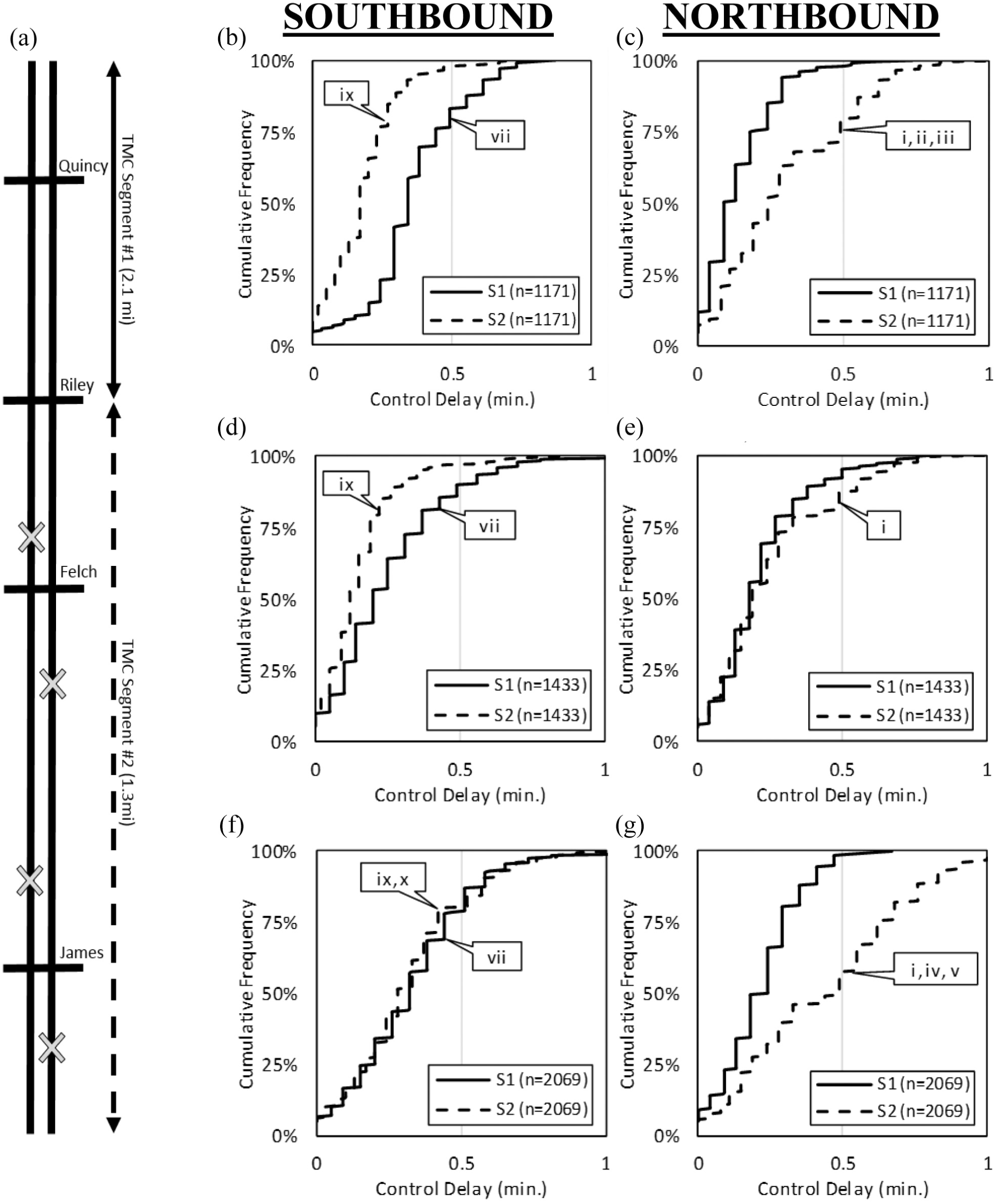
Five sensors were used on the US-31 corridor in Holland. The placement of these sensors relative to the signalized intersections can be seen in Figure 3a. Using these devices, a week’s travel time data were collected between June 19th and June 23rd, 2017. The 15th percentile travel time was used as a baseline travel time, and cumulative distribution functions were created as a measure of control delay for each timing plan and direction. The 15th percentile was chosen to eliminate outliers that may have represented cyclists, pedestrians, or vehicles stopping on the corridor. These results are visualized in Figure 3. The numbers of Bluetooth/Wi-Fi devices used in each of the cumulative distribution function (CDF) lines are provided in the legends.
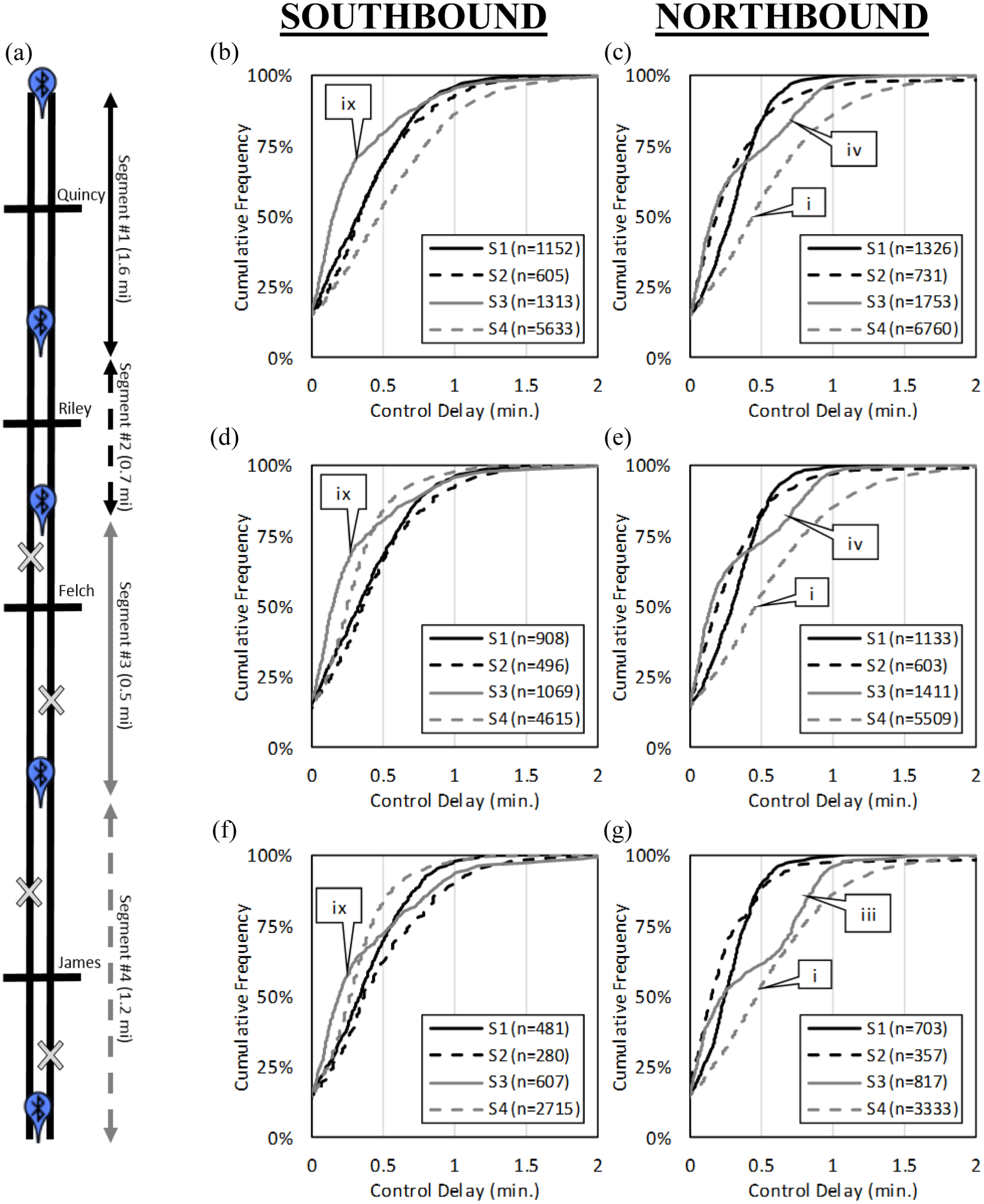
Control delay of probe segments using Bluetooth/Wi-Fi sensors, showing (a) map of the US-31 corridor, and results for (b) SB 05:00–09:00, (c) NB 05:00–09:00, (d) SB 09:00–14:00, (e) NB 09:00–14:00, (f) SB 14:00–21:00, and (g) NB 14:00–21:00.
The signal timing issues previously observed in Figure 2 are again pointed out in the CDFs in Figure 3. In CDFs, a more vertical line represents higher reliability and a more horizontal line represents less reliable travel times. For example, in Figure 3, callout “i” shows random arrivals at the South James crossover, which manifests as a uniform control delay distribution, represented by a sloped CDF. Additionally, the offset issues at Felch and the South Felch crossover induce characteristic variations in control delay in Segment 3 (Figure 3, callouts “iv” and “iii”). The SB direction has little disparity amongst the control delay distributions. However, the slight variation in Segment 3 (Figure 3, callout “ix”) represents the left-turning vehicles from Riley that are not arriving on green.
Overall, the probe travel data collected via Bluetooth/Wi-Fi sensors can be used to identify significant deficiencies in coordinated signal timing. But although the data can locate issues, they are less useful for suggesting potential offset adjustments. The data have some inherent limitations. Vehicle re-identification does not guarantee that the device is taking the most direct approach to the next sensor, or that the device represents a motor vehicle (i.e., it could potentially be a pedestrian or bike). The sensors have the advantage of being mobile; therefore, the segments can be customized for each corridor. However, non-midblock installations could potentially skew the data by detecting queued vehicles on the side streets.
Segment-Based Probe Vehicle Data
Commercial probe vehicle data are amongst the most widely used sources for mobility and travel time data. In this study, segment-based travel time data were used to create cumulative distribution function graphics of control delay to determine whether signal coordination issues could be discovered. Data from the week of June 19, 2017 were used. The traffic message channel (TMC) segmentation scheme was used. This scheme included two segments encompassing the signals on the corridor of interest. Because the segment-based data contain fewer outliers as a result of their aggregation to the nearest minute, the 5th percentile travel time was used as the baseline for the control delay diagrams in Figure 4. This differs from the 15th percentile used in the Bluetooth/Wi-Fi control delay diagrams because the segment-based data has eliminated a majority of outliers in the initial data aggregation. The numbers of minutes used in each of the CDF lines are provided in the legends.
Control delay of probe segments using crowdsourced probe data, showing (a) map of the US-31 corridor, and results for (b) SB 05:00–09:00, (c) NB 05:00–09:00, (d) SB 09:00–14:00, (e) NB 09:00–14:00, (f) SB 14:00–21:00, and (g) NB 14:00–21:00.
The entire signalized portion of the corridor is represented in two segments. Having only two segments for a span of several intersections makes locating specific signal issues difficult. However, the data do reveal coordination problems. In the NB direction, during the a.m. and p.m. timing plans, Segment 2 has noticeably higher delay than the midday plan. This corresponds to offset deficiencies revealed by the PCDs (Figure 2). In the SB direction, random arrivals at Quincy are clearly visible in all three timing plans. The p.m. plan in the SB direction also shows a more severe issue in Segment 2, corresponding to the offset deficiency at the North James crossover.
In summary, segment-based probe data can be used to identify problems with signal coordination, but because of the broad spatial and temporal aggregation of the data, it is difficult to determine the intersection where the deficiencies are occurring, or the specific deficiency that is taking place.
Automated Vehicle Location Trajectory Data
The final approach used is a relatively new data source. The same commercial providers of the segment-based data are now providing raw data that allow for the creation of individual vehicle trajectories. The AVL trajectory data set contains anonymized unique vehicle trip identifiers, timestamps, waypoints, latitudes, and longitudes. Over a 2-week period 10,466 unique vehicle IDs were recorded with a total of 109,879 unique pings. Assuming the highest AADT as the entering volume of the corridor, approximately 1.8% of vehicles were recognized. A Structured Query Language (SQL) server was used to create a spatial reference point to organize the geospatial data. This reference is referred to as the origin. Vehicles traveling the entire stretch of road were selected and grouped together into a single data set. From this, 702 unique vehicle IDs with 45,539 pings were found to travel the entire corridor. The remaining data were processed using MATLAB to calculate the distance from the origin along the defined roadway and the elapsed trip time. This allowed for both straight and curved roadways to be assessed. The MATLAB script removed trips with fewer than 10 pinged locations, and pings greater than 5 s apart. The filtering of infrequent pings resulted in 235 unique vehicle trips with 34,663 pings over a 2-week period. These points were then plotted as vehicle trajectories (Figure 5a). This data source is rich for use in transportation engineering and operations. However, the high volume of data makes it challenging to manage.
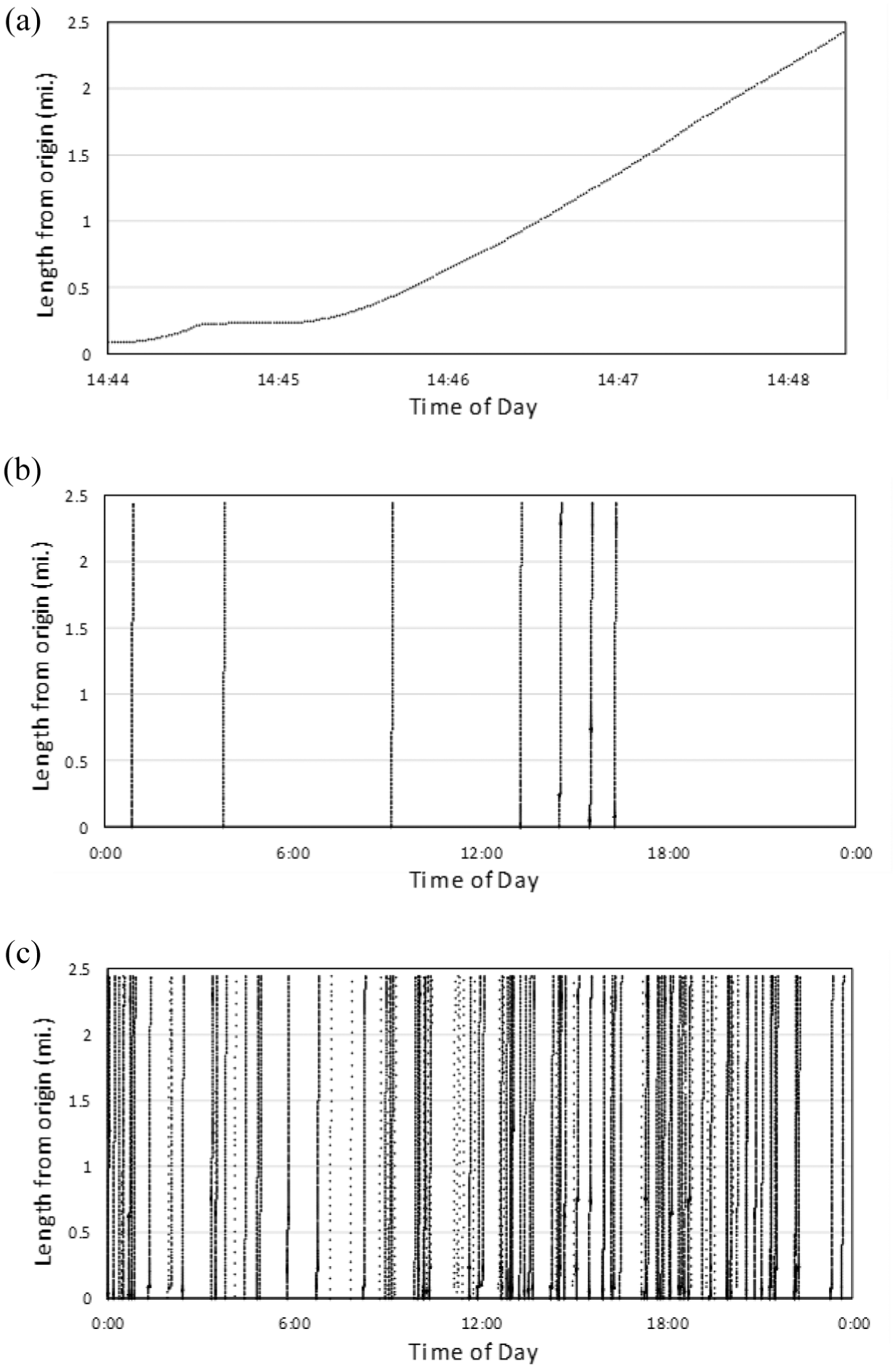
Vehicle trajectory aggregation on NB US-31, showing (a) single AVL trajectory, (b) single day of AVL trajectories (7/3/2017), and (c) 2 weeks of aggregated trajectories (6/30–7/14/2017).
For this analysis, only probe vehicles that traversed the entire corridor were included to measure coordination from start to finish. Shorter segments will be used later to assess individual intersection performance. In addition, any trips for which the time between pings exceeded 5 s were excluded. Consequently, relatively few individual probe vehicle trip records were retained for any given time period. To counter this, the data were aggregated over a longer time period. Figure 5b shows a single day of probes traveling the corridor, and Figure 5c shows 2 weeks (6/30–7/14/2017) of trajectories overlaid onto a single day. These trajectories were then aggregated on a single point on the corridor and plotted to create a visualization of corridor progression. Figure 6a shows the SB direction and Figure 6b shows the NB direction. As was previously observed, progression in the SB direction is obviously superior to the NB direction because more NB trajectories exhibit control delay represented by horizontal segments on the trajectory. Additionally, the distribution of trajectory points exhibiting optimal progression outnumbers the trajectory points exhibiting poor progression, which may cause a misinterpretation of coordinated corridor performance. Supplemental numerical representation may be required to truly quantify performance.
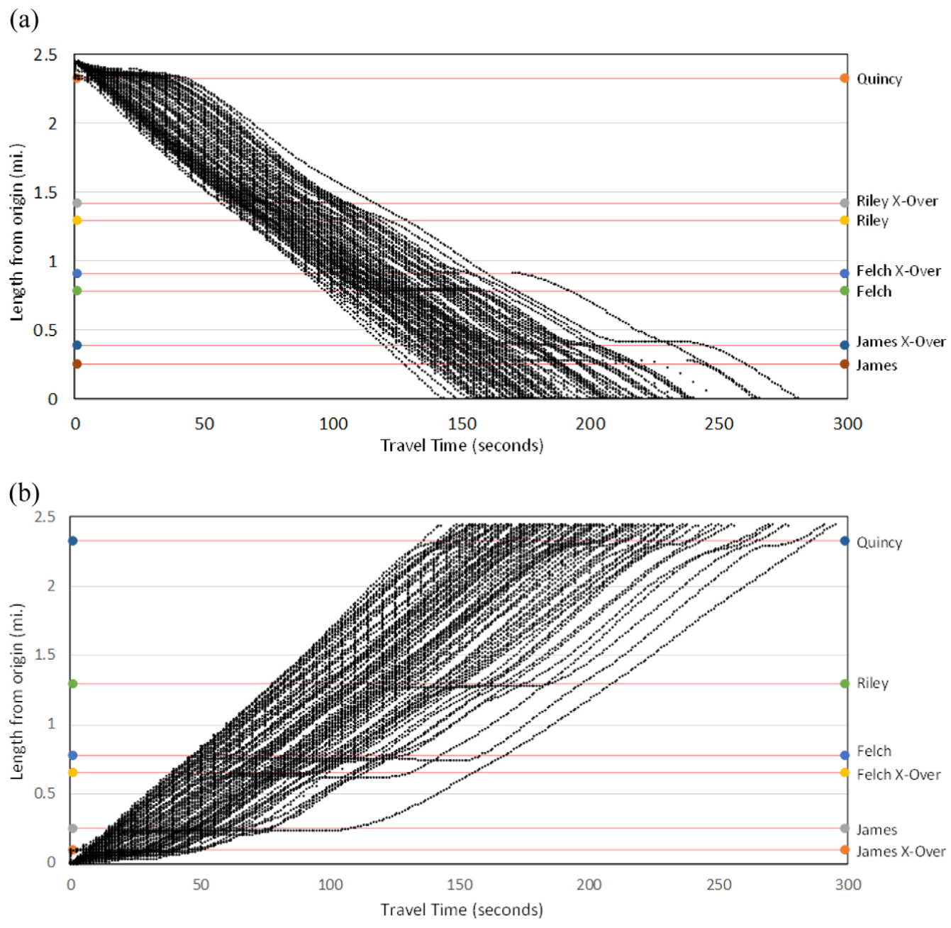
Aggregated corridor level vehicle trajectories, showing (a) SB trajectory data (2 weeks) and (b) NB trajectory data (2 weeks).
To make better sense of it, the trajectory data can be broken down by timing plan (Figure 7). The a.m. timing plan in the NB direction (Figure 7a) had few probes to visualize, but one of the three did stop at both the South James crossover and James, which could reflect the issue shown in the PCD (Figure 2, callout “ii”). The midday timing plan in the NB direction appears not to have any issues, using the trajectory data in Figure 7b. This is also in agreement with the PCDs in Figure 2. Figure 7c shows the p.m. timing plan for the NB direction. There were clearly issues in the PCD at the Felch crossover/Felch (Figure 2 callouts “iv” and “v”) and at Quincy Street (Figure 2 callout “vii”). These issues are also observable in Figure 7c, callouts “i” and “ii”, respectively. Unsurprisingly, the trajectory data is a useful source to monitor corridor progression. Such data is frequently used in floating car studies in current practice. However, by crowdsourcing the data collection, a much broader time period can be captured.
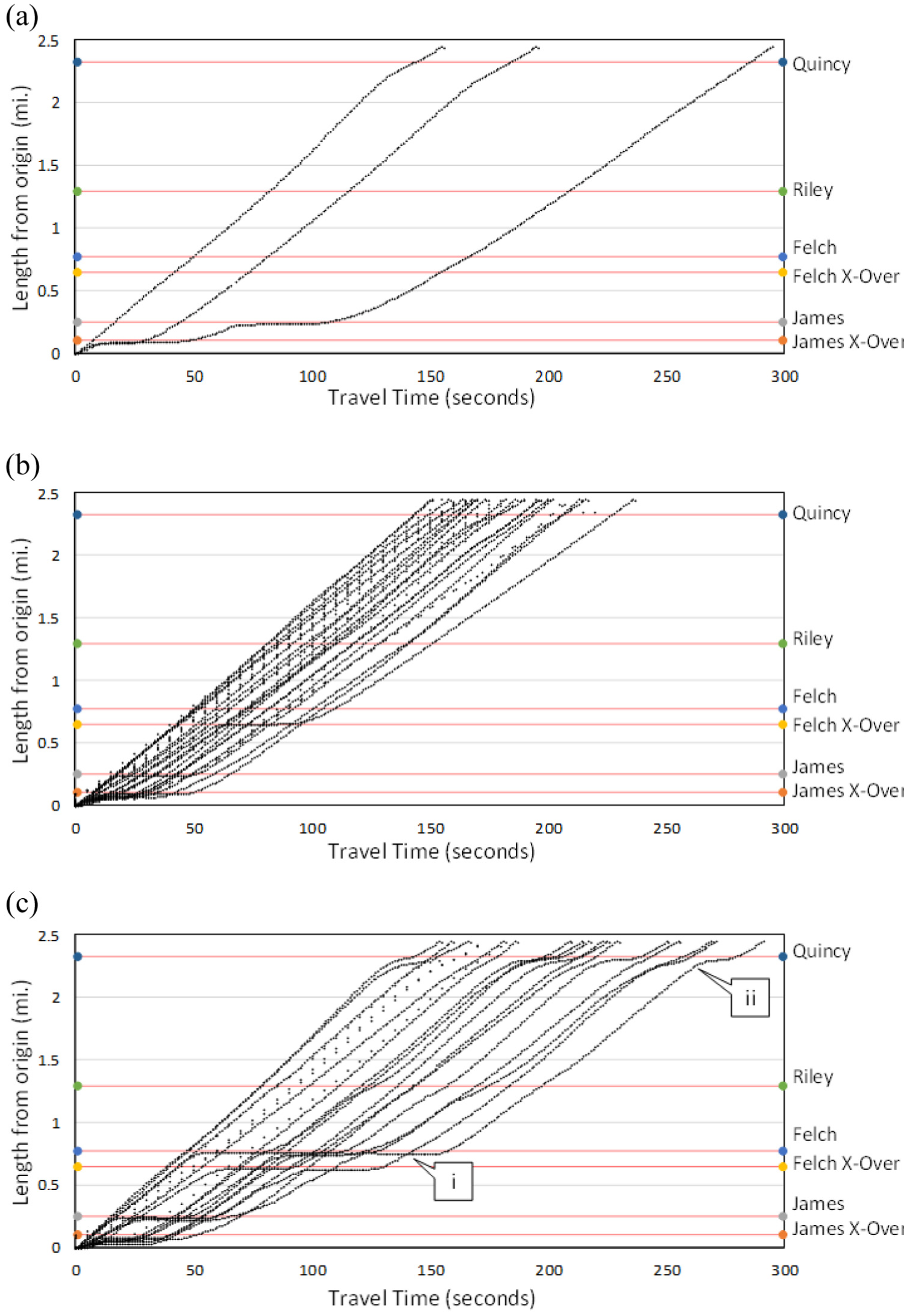
Vehicle trajectories by timing plan, showing (a) Timing Plan 1 (05:00–09:00), (b) Timing Plan 2 (09:00–14:00), and (c) Timing Plan 3 (14:00–21:00).
The trajectory data can also be used to estimate arrivals on green. A similar approach to the corridor trajectory strategy was used to create intersection-based graphics. Figure 8 shows three intersections on the US-31 corridor with the corresponding PCD. Figure 8a shows the NB Riley intersection. This approach operates well, with a daily percentage on green (POG) of 86.7% according to the detector data. Using trajectory data, a POG of 93% is calculated. Figure 8b shows the NB James intersection, which has an offset issue in the AM period. The detector-based POG is 82.4%, whereas trajectory data yields a POG of 80%. Figure 8c shows the SB Quincy intersection, which has random arrivals as it is on the end of the corridor. The detector POG is 64.4%, whereas the trajectory POG is 60%.
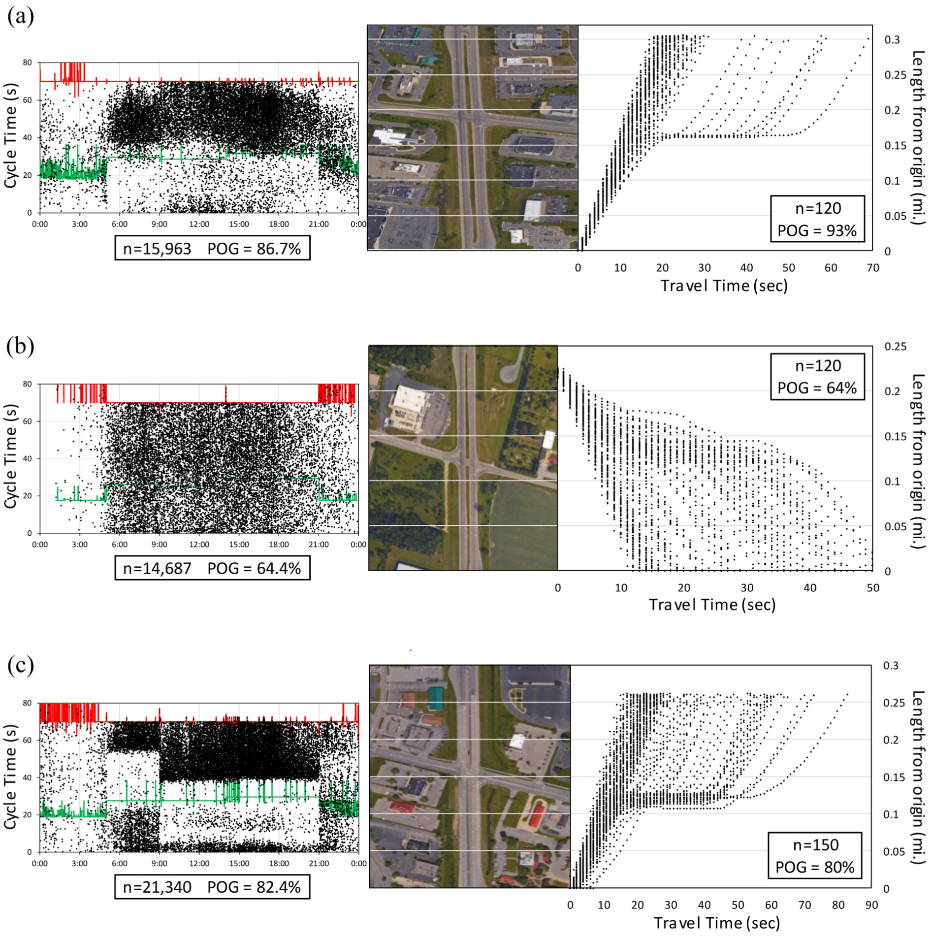
Arrival pattern comparison between PCD and trajectory data, showing (a) NB Riley Street, (b) NB James Street, and (c) SB Quincy Street.
There is some variance between these two POG numbers, but the former represents 1 day of detections whereas the latter comprises 2 weeks of trajectories. Nevertheless, the figures appear to correlate in this initial exploration. There is likely some promise for use of trajectory data to create infrastructure-free performance measures. Figure 9 further demonstrates the scalability of an analysis strategy based on trajectory data. A corridor in Columbus, Ohio was analyzed using trajectory data. The authors had no knowledge of the corridor before acquiring the data. Trajectory diagrams were created for WB OH-750 and EB OH-750. Aerial imagery was used to determine the signal locations for these charts. However, even if those locations were not explicitly shown in the charts, coordination issues would be apparent. The westbound (WB) direction (Figure 9a) has fewer, but rather long stops; the eastbound (EB) direction (Figure 9b) shows many numerous stops on practically every trajectory.
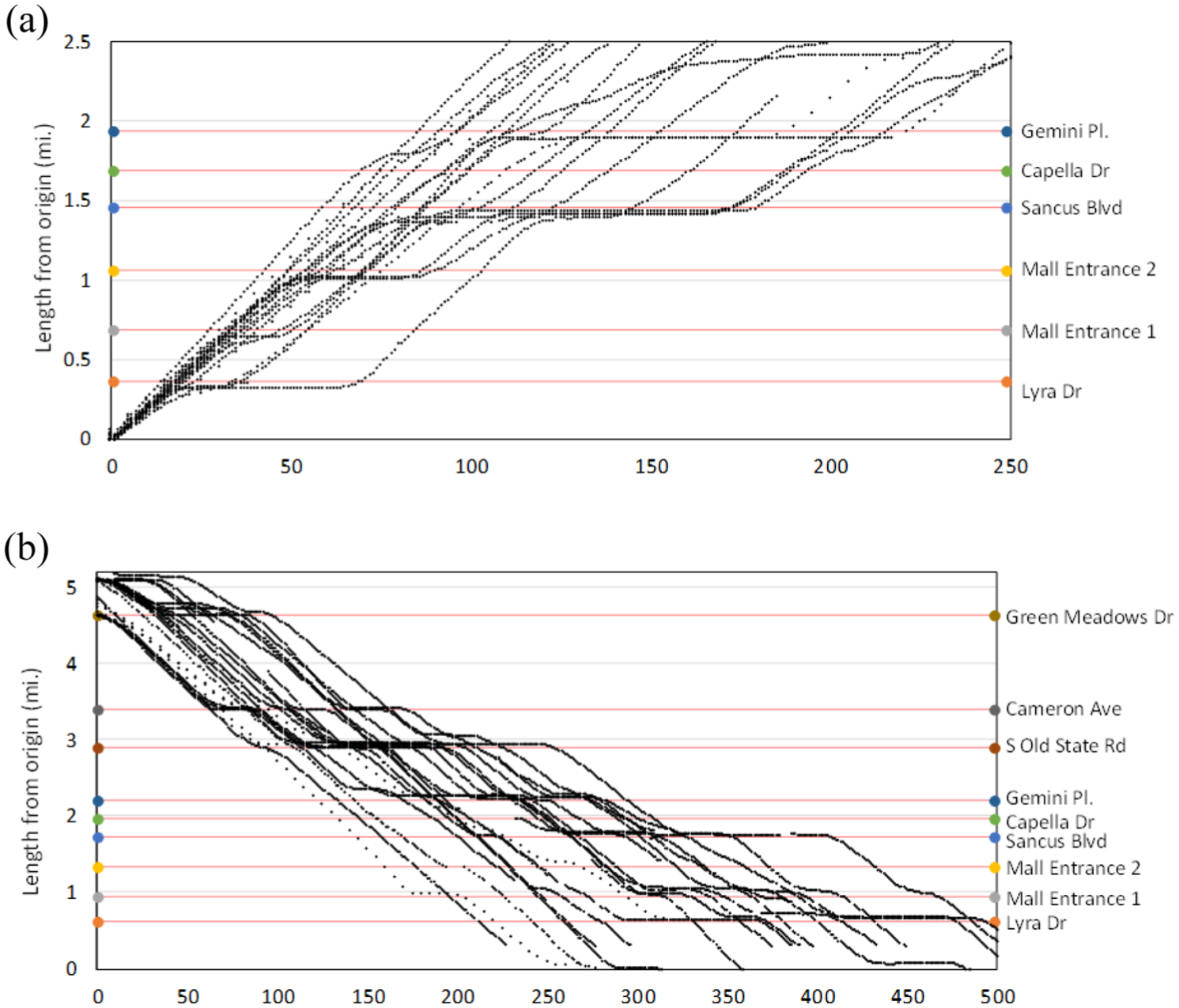
OH-750 signalized corridor in Columbus, Ohio, showing (a) portion of WB OH-750 and (b) portion of EB OH-750.
In addition, these trajectory diagrams can be fused with controller data to create composite time space diagrams. Such diagrams were created for the Holland corridor, as shown in Figure 10. The SB direction (Figure 10, a–c ) shows stops at Quincy (callout “i”), Felch (callout “ii”), and James (callout “iii”). The NB direction shows stops at James crossover (callout “iv”), James (callout “vi”), and the Felch crossover (callout “v”). This information could potentially be used to validate software-based timing plans immediately after field implementation, rather than waiting for user complaints.
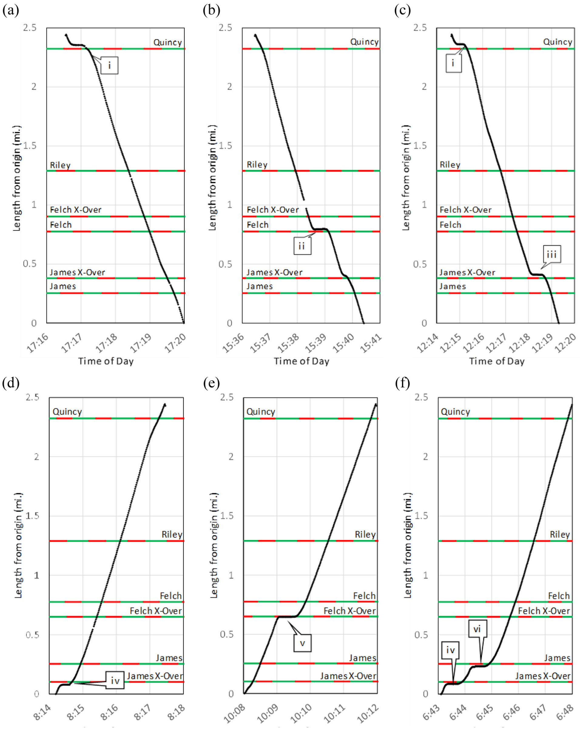
Fusion of high-resolution controller data and probe trajectory data, showing (a) SB Trajectory 1 (7/11), (b) SB Trajectory 2 (7/11), (c) SB Trajectory 3 (7/12), (d) NB Trajectory 1 (7/13), (e) NB Trajectory 2 (7/12), and (f) NB Trajectory 3 (7/10).
Similar data fusion strategies have been executed with floating car data ( 1 ); however, crowdsourcing such data can greatly reduce the labor required to obtain the data. These charts demonstrate that it is possible to do so with commercial trajectory data. It had been speculated that clock synchronization would present a formidable challenge in such data fusion, but the data in Figure 10 do not exhibit the types of anomalies that were anticipated, such as vehicles stopping on green or proceeding on red. This agrees with the previous comparison of detector and trajectory arrival profiles ( 17 ), suggesting that as long as the controller data is updated using a common time server, clock synchronization is unlikely to prove an Achilles’ heel for data fusion between controller and vehicle data.
Conclusions
The assessment of signal coordination is a demanding effort that has historically relied on traditional measures, such as user complaints and individual travel runs. Recently, numerous technologies have been developed that can assist with the assessment of coordination. Both segment-based probe data and Bluetooth/Wi-Fi sensors can be used to detect if there are any issues; however, the ability of that data to suggest changes is limited. Bluetooth/Wi-Fi requires the purchase of infrastructure, but the corridors are customizable. Segment-based probe data requires no permanent infrastructure, but the segments are predefined, and may span numerous signals. As more agencies have purchased segment-based probe data for evaluating traffic operations, the cost of historical data has come down. Bluetooth sensors still require infrastructure and maintenance costs, generally requiring more of an investment than segment-based probe data. Segment-based analysis with Bluetooth/Wi-Fi sensors or probe data may be useful in problem identification with more intensive and costly evaluation, such as trajectory based methods, to be used in development of refined signal timing approaches.
Detector-based signal performance measures are excellent tools for measuring signal performance and adjusting signal timings. The data can identify issues and can be used to optimize coordination on a corridor ( 3 ). However, if there is no existing advanced detection on a corridor, a substantial investment is needed to acquire this data. If detection is present (as would be common for actuated-coordinated operation), the costs may be reasonable, depending on the abilities of the traffic controller and communication between the cabinet and an operations center. At the time of writing, six different controller manufacturers had at least one controller model with the capability of logging high-resolution data ( 20 ). In addition, several third-party products have emerged to add that capability to locations with legacy equipment.
Crowdsourced trajectory data can also be used to identify coordination issues, and adjust offsets to address those issues. No permanent infrastructure is required to collect this information; however, the temporal coverage is currently limited. This requires data aggregation over time to develop useful performance measures. The spatial coverages of these vehicle trajectories are limitless. At present, because this is a new data source, the costs are high. This is an economy-of-scale issue. As more agencies purchase the data, and the population of probe vehicles increases, the cost per data point will decrease. In the future, these data sources can be used to create aggregate performance metrics, such as average control delay, and to compare various corridors.
In future research, larger periods of time will be used for each of the data sets to truly compare data accuracy. These data can then be used to develop aggregate corridor performance metrics for agency use to prioritize signal improvements. Connected vehicle data based on DSRC may provide another path to the same type of data. However, because of privacy concerns, such data may only be available within close proximity of individual intersections; connecting trajectories along corridors might not be feasible. In summary, the future of vehicle trajectory data is very promising, with potential use cases for planning, operations, maintenance, and rapid validation of the models used in those endeavors.
Footnotes
Acknowledgements
The vehicle trajectory data provided in this paper were provided by INRIX. Signal performance measure data for this paper were provided by an ongoing research project with the Michigan Department of Transportation.
Author Contributions
The authors confirm contribution to the paper as follows: study conception and design: Remias; data collection: Wadell, Kirsch, Trepanier; analysis and interpretation of results: Remias, Day, Wadell, Kirsch; draft manuscript preparation: All. All authors reviewed the results and approved the final version of the manuscript.
The Standing Committee on Traffic Signal Systems (AHB25) peer-reviewed this paper (18-03728).
The contents of this paper reflect the views of the authors, who are responsible for the facts and the accuracy of the data presented here, and do not necessarily reflect the official views or policies of the sponsoring organizations. These contents do not constitute a standard, specification, or regulation.