Validation and Calibration of Freeway Reliability Methodology in the Highway Capacity Manual: Method and Case Studies

Abstract

Traffic congestion costs drivers an average of $1,200 a year in wasted fuel and time, with most travelers becoming less tolerant of unexpected delays. Substantial efforts have been made to account for the impact of non-recurring sources of congestion on travel time reliability. The 6^th edition of the Highway Capacity Manual (HCM) provides a structured guidance on a step-by-step analysis to estimate reliability performance measures on freeway facilities. However, practical implementation of these methods poses its own challenges. Performing these analyses requires assimilation of data scattered in different platforms, and this assimilation is complicated further by the fact that data and data platforms differ from state to state. This paper focuses on practical calibration and validation methods of the core and reliability analyses described in the HCM. The main objective is to provide HCM users with guidance on collecting data for freeway reliability analysis as well as validating the reliability performance measures predictions of the HCM methodology. A real-world case study on three routes on Interstate 40 in the Raleigh-Durham area in North Carolina is used to describe the steps required for conducting this analysis. The travel time index (TTI) distribution, reported by the HCM models, was found to match those from probe-based travel time data closely up to the 80^th percentile values. However, because of a mismatch between the actual and HCM estimated incident allocation patterns both spatially and temporally, and the fact that traffic demands in the HCM methods are by default insensitive to the occurrence of major incidents, the HCM approach tended to generate larger travel time values in the upper regions of the travel time distribution.

Increasing traffic congestion and driver frustration on urban freeways have been the motivation behind several studies related to travel time reliability. Most travelers are less tolerant of unexpected delays because they have larger consequences than everyday congestion ( 1 ). Traffic jams cost drivers in the U.S. an average of $1,200 a year in wasted fuel and time, according to a study by INRIX ( 2 ). Travel time reliability is an important performance measure used to describe travel characteristics on freeways and urban streets. It is used to quantify variability in travel time, which can be a result of both recurring and non-recurring congestion such as inclement weather or incidents. Recent federal rulemakings published by the Federal Highway Administration (FHWA) have proposed that reliability performance measures be used as a basis for federal funding prioritization of road projects ( 3 ).

Substantial efforts have been made to account for the impact of non-recurring sources of congestion on travel time variation. The Highway Capacity Manual (HCM), one of the most widely used references used by analysts for evaluating capacity and level of service on freeways, also provides methods to account for the impact of non-recurring sources of congestion ( 4 ). Chapters 11 and 17 of the latest release of the manual contain a methodology for travel time reliability analysis for freeways and arterial streets. This entails expanding the analysis window from a few hours on a single day to a whole year. Non-recurring sources of congestion such as inclement weather, incidents, and work zones are accounted for within this wider window. By default, the HCM freeway reliability methodology generates 240 scenarios (roughly equivalent to the number of work weekdays in a year) to simulate variations in demand, weather, and incident events throughout the year ( 5 ).

A key prerequisite to carrying out a reliability analysis is a single day (or seed day) calibration of the facility being analyzed. The seed-day scenario is then augmented to include recurring (demand) and non-recurring sources of congestion, thus generating new and different sets of scenarios. As the goal is to represent real-world operating conditions on the facility, all sources of congestion must also be calibrated using field data. This can be done through matching the likelihoods of events like incidents, severe weather, work zones, and so forth, in the model to actual observations and their impact on travel time.

The 6^th edition of HCM provides structured guidance on a step-by-step calibration of the core (single day) as well as reliability analysis, as displayed in Figure 1. However, practical implementation of these methods requires collecting data scattered in different platforms and available in inconsistent formats. The most widely used data source to calibrate the core analysis are probe-based speed data (e.g., from INRIX, HERE). The reliability calibration requires weather information daily incident frequencies, which must be extracted and filtered for errors, omissions, and outliers, all of which can affect the incident frequency estimations.

Figure 1.

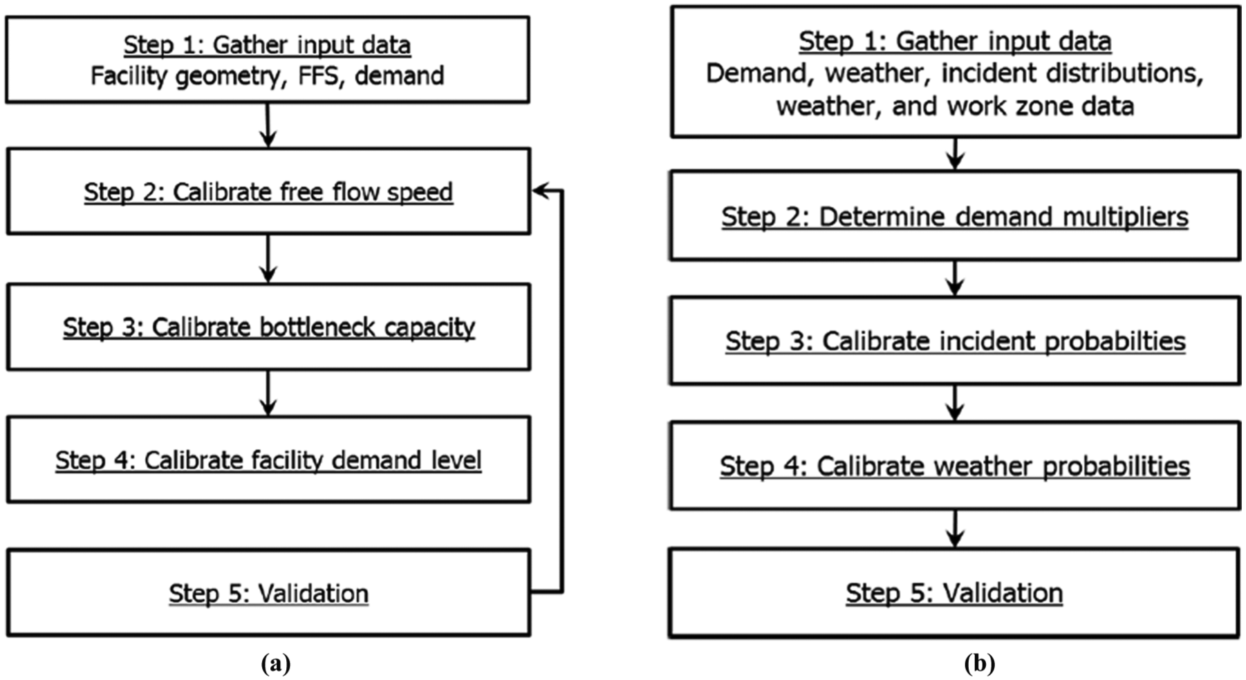
Calibration process for freeway core and reliability analysis in HCM ( 4 ). (a) HCM exhibit 25-26 core analysis calibration procedure; (b) HCM exhibit 25-32 reliability calibration procedure.

This paper focuses on the calibration and validation of both the core (single day) and reliability analyses in HCM ( 4 ). The main objective is to provide HCM users with guidance on collecting data for freeway reliability analysis and validating the reliability performance measures predictions of HCM models. An extensive review of research pertaining to travel time reliability modeling is provided, and the process for collecting and pre-processing the inputs required for such analysis is explained. The output of reliability analysis in the HCM method is then validated using a case study on Interstate 40 near Raleigh-Durham, NC.

Literature Review

Travel time reliability includes the notion of predictability, that is, the probability that the travel time on a facility is within acceptable limits for the traveler, given that travel times are affected by interaction of demand fluctuations, traffic control devices, traffic incidents, inclement weather, work zones, and physical capacity. A variety of performance measures have been proposed to quantify reliability, which include 80^th percentile travel time, travel time index (TTI), planning time index (PTI), buffer time index, and many others. The use of an indexed term like TTI or PTI is generally preferred as it normalizes the travel time by the free-flow travel time on the facility, which enables easier comparison across facilities. Among these measures, a National Cooperative Highway Research Program effort identified the Buffer Time Index as the most useful reliability performance measure, including a successful field test by four U.S. transportation agencies ( 6 ). Franklin modeled reliability as expected lateness using a schedule-based approach ( 7 ). The study examined travel time data for mean lateness, an important component of scheduling, to produce a complete estimate of user benefit.

Rakha et al. investigated the relationships between segment and trip travel time reliability metrics, and explored and validated options for characterizing trip reliability ( 8 ). Through another large national research effort conducted under the SHRP-2 L03 project, many reliability performance measures and macroscopic methods for estimating key reliability measures from average travel times were proposed ( 9 ). Studies have investigated the impact of stochastic bottleneck capacity on reliability ( 10 ) and even extended to estimating travel time distribution based on demand and capacity ( 11 , 12 ).

Traffic demand variations, inclement weather conditions, and incidents are recognized as principal factors affecting the variability of travel times on the freeways ( 13 , 14 ). Presence of construction zones have been studied as one of the sources of non-recurring congestion. Al Kaisy and Hall developed guidelines for estimating freeway capacity at long-term reconstruction zones ( 15 ), and Krammes and Lopez ( 16 ) did the same for short-term freeway work zones. Chituri et al. ( 17 ) and Schroeder and Rouphail ( 18 ) extended those analyses to include delay and user costs for freeway work zones.

Similarly, several researchers have studied the impact of weather on non-recurring congestion. A change in weather conditions can affect the capacity and the free-flow speed of the freeway, resulting in changes in travel time ( 13 , 19 ). The occurrence of different weather conditions is difficult to predict, but their expectancy could be estimated based on historical averages ( 20 ). Rakha et al. proposed specific adjustments to traffic flow parameters based on specific weather events ( 21 ). Similar work on the effects of rainfall and other environmental factors on traffic flow characteristics on urban freeways have been reported by Shi et al. ( 22 ), whereas Dehman ( 23 ) focused on the effect of inclement weather on both capacity and queue discharge headways at recurring freeway bottlenecks.

The occurrence of incidents is stochastic in nature and can result in a reduction in the capacity and/or speeds ( 4 , 13 , 24 ). Moreover, the location, severity, and duration of an incident can altogether influence its impact on the facility travel time. Skabardonis et al. showed that incident occurrence on a freeway facility follows the Poisson distribution ( 25 ). However, more detailed research has suggested that incident occurrence follows a binomial distribution and that incident counts are much more dispersed, with variance greater than the mean ( 14 ). Research involving distribution of duration of incidents on freeways assumes that it closely follows a Lognormal or a Gamma distribution ( 14 ).

From the literature, it is evident that weather, work zones, and incidents are all likely to have significant impact on freeway capacity, free-flow speeds, or in many cases both. The latest version of HCM comes with a revised method to generate reliability scenarios and calculate performance metrics, primarily TTI distributions. However, validations conducted as part of the SHRP 2 L08 project revealed that the observed capacity values in the field were usually lower than the proposed values in the manual ( 26 – 30 ).

During the core facility calibration, if an unwanted bottleneck appeared in the model, the guidance recommends increasing the capacity of a segment until it disappears. Beyond this, the HCM provides no insight on how to adjust capacity and match predicted speeds to field-observed speeds. Therefore in many cases, the capacity calibration process becomes a trial-and-error process until a satisfactory level of accuracy is achieved. A new optimization-based approach for bottleneck calibration on freeway facilities, in the context of the HCM analysis, uses a genetic algorithm to adjust segment demand and capacity to match HCM-modeled and observed speeds predicted at a high level of confidence ( 31 ).

Methodology

This section of the paper discusses the implementation of both the core and reliability analyses in the HCM, along with the application of the proposed methodologies on three selected study routes.

Site Selection

The temporal and spatial boundaries of the study routes were carefully considered in order to capture daily recurring congestion patterns as well as all seasonal travel trends. Two freeway sections on I-40 in the Raleigh-Durham area in North Carolina, selected for reliability analysis, are shown in Figure 2.

Figure 2.

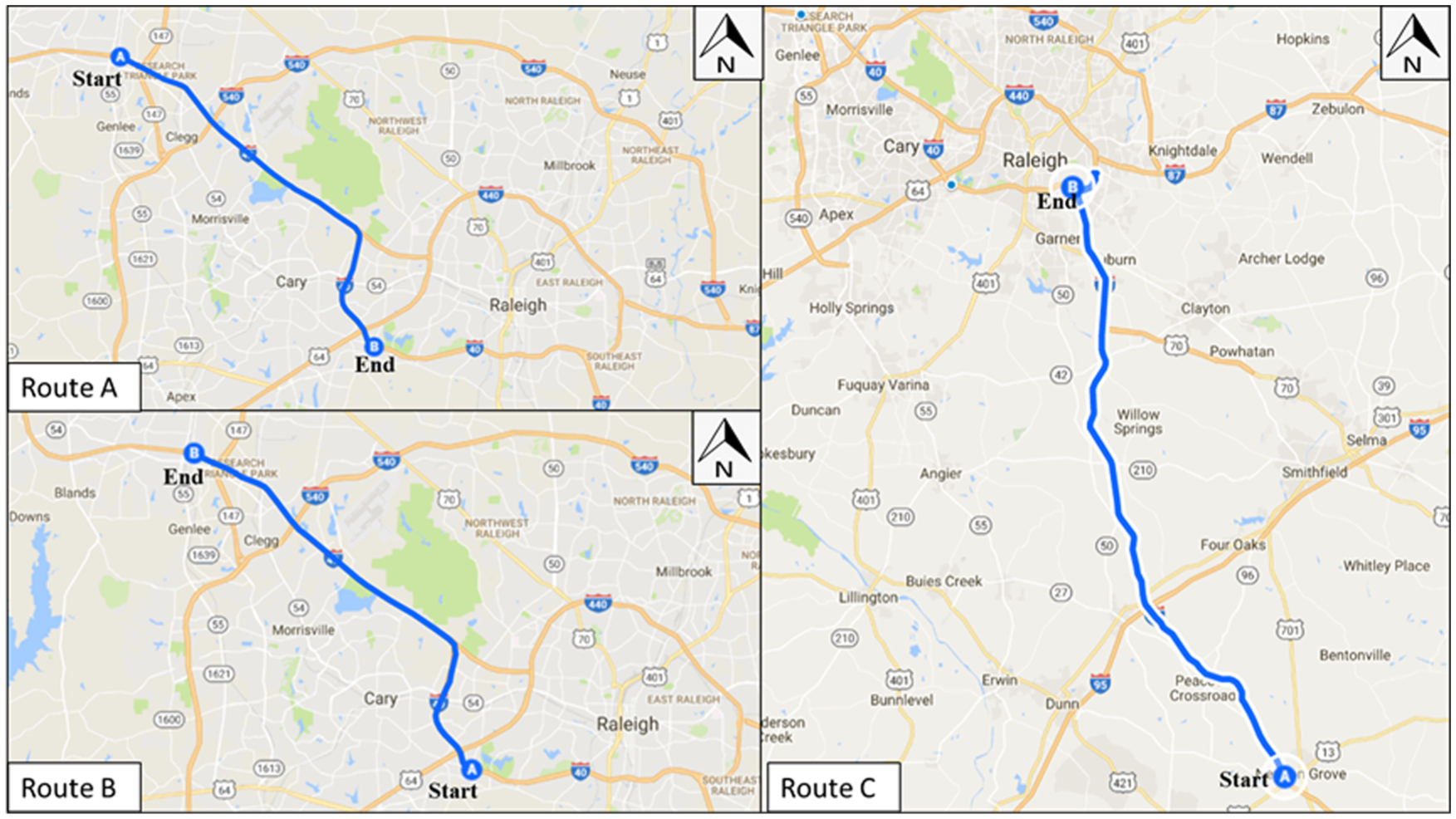
Directional (A→B) freeway facilities analyzed.

Route A, an urban interstate route, is 14.72 miles long along I-40 Eastbound from US-1 to NC-147, contains 23 traffic message channel (TMC) segments, and experiences a morning peak demand. It is primarily a commuter route that passes through the Research Triangle Park, a major employment center in the area and has a speed limit of 65 mph along the entire path. Route B is the westbound direction of travel on this route, with a p.m. peak travel. Route C, an exurban/ rural interstate, is 39.84 miles long on I-40 WB from NC-50/55 to I-440 and contains 17 TMC links. The path crosses I-95 on the way to Raleigh, NC from southeastern North Carolina. The speed limit is 70 mph from the origin until approximately 30 miles into the path, where the speed limit drops to 65 mph for the remainder of the path. This route experiences an a.m. peak commuting period. A study period of 24-hour and a reliability reporting period included all weekdays for the year 2015.

Core Methodology Calibration and Modeling

This section discusses the steps needed to calibrate the core facility (see also Figure 1a).

Step 1: Facility Geometry

The first step involves defining the segments’ geometry consistent with the requirements of performing the analysis method described in the HCM. In this study, routes A, B, and C consist of 37, 45 and 37 HCM segments, respectively, per the HCM guidelines on segmenting freeway facilities. Other inputs such as segment length, number of lanes, shoulder clearances, and so forth, were extracted directly from Google Maps.

Step 2: Calibrate Free-Flow Speed

Travel times at very low traffic demand conditions represent free-flow travel times, as a direct function of free-flow speed. The estimated free-flow travel times at low traffic demand flows were compared with the probe-based sensor data and necessary adjustments were made to calibrate the free-flow speed in the models.

Step 3: Calibrate Bottleneck Capacity

An automated approach for the HCM bottleneck capacity calibration process was used in this step ( 31 ). It involves mathematical optimization, using a genetic algorithm metaheuristic to estimate capacity adjustment factors and identify facility. It optimizes the capacity adjustments such that they result in predicted performance measures consistent with the collected empirical speed data and significantly helps reduce the time and effort needed for analysis.

Step 4: Calibrate Facility Demand Level

Demand flow rates for the mainline, on-ramp entry, and off-ramp exit were estimated based on annual average daily traffic (AADT) and hourly demand profiles, and subsequently aggregated into 15-minute intervals. Collectively, this forms the basis of the input for the model.

Step 5: Validation

The primary data source for calibration was INRIX (extracted from RITIS.org), which provides probe-based travel time and speed data ( 32 ). Several days’ worth of data were gathered, and outlier days, such as days with unusual congestion patterns or no congestion, were excluded from the dataset. INRIX uses internal and external TMC codes as the smallest spatial unit for reporting freeways performance measures. This method reports traffic data between each break in access on any road (such as from one on-ramp to next off-ramp). It was observed that a single TMC segment usually covers two or more HCM segments, as per the example shown in Figure 3.

Figure 3.

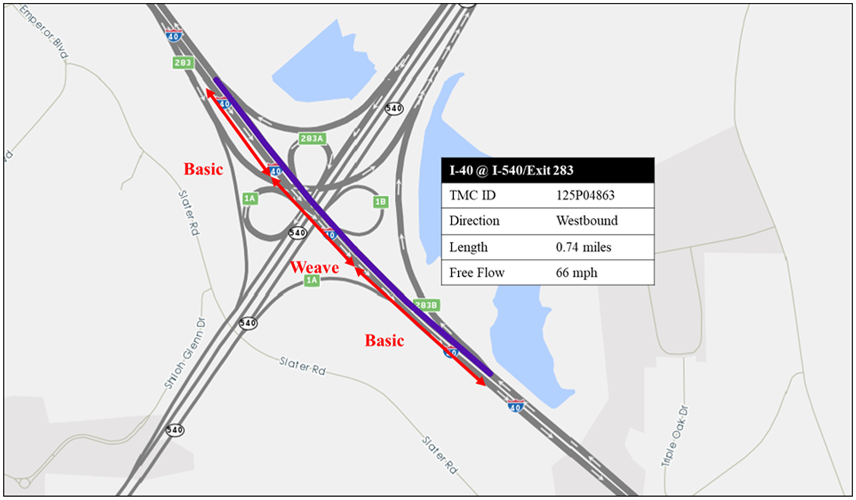
An INRIX TMC segment on WB I-40 (in purple) containing 3 HCM segments (in red) at the interchange with I-540.

To perform validation via probe-based data sources, the actual facility as configured was converted into HCM segments. A length-based average of HCM segments’ performance measures is used to match TMC segments. Thus, if a TMC segment contains n HCM segments of length L_i each, then the aggregated travel time performance measure is computed as:

T T_{TMC} = \frac{\sum_{i = 1}^{n} L_{i} \times T T_{HCM, i}}{\sum_{i = 1}^{n} L_{i}}

(1)

Where $T T_{TMC}$ is travel time on TMC segment and $T T_{HCM}$ is travel time on HCM segment.

Equation 1 was used to match the performance of TMC and HCM segments. This process provided the basis for comparing the HCM reported performance measures with TMC segment observations.

Reliability Analysis Calibration and Modeling

After the core calibration of the three selected facilities, calibration for the reliability scenarios was performed. As stated in HCM Chapter 11, characterization of the demand fluctuation across days of the week and months of the year, along with calibration of non-recurring congestion sources, that is, incidents, weather, work zones, and so forth ( 4 ). The following steps are based on Figure 1b.

Step 1: Gather Input Data

The types of data required for calibration of reliability analysis include demand, weather, incident distributions, and work zone data, as shown in Figure 1b. Chapter 11 of the HCM also provides information for data requirements for agencies with low access to good quality data ( 4 ). The best source of demand fluctuation data is permanent traffic recorders located alongside the facility. Demand multipliers are a direct input into the HCM model and represent the ratio of the traffic demand in each analysis period to the AADT. Those are then used to generate the input demand level for each scenario. Calibrating weather events requires historical weather data, which were gathered from the Weather Underground website. For modeling the effect of incidents, detailed incident logs are needed, which were collected from incident management websites managed by North Carolina Department of Transportation (NCDOT). It should be noted that the study sites in this paper did not have any on-going construction zones during the year 2015.

Step 2: Determine Demand Multipliers

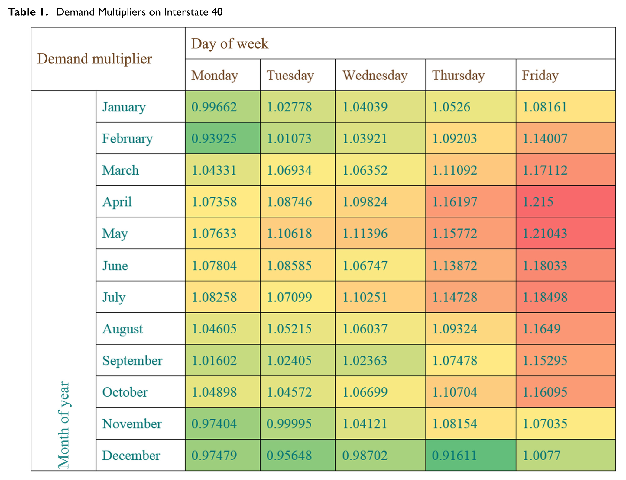
Demand level should be studied for the facility where the reliability analysis is performed ( 13 ). Categorization of demand is done by assigning similar demand patterns to specific days with the same demand level in the reliability scenario generator. Demand patterns are defined along two dimensions, accounting for monthly and weekday variability. Monthly variability accounts for seasonal trends in travel, whereas the weekday dimension shows the effect of day-to-day variation in demand. These demand multipliers give the ratio of demand for a day–month combination to the AADT, and are used to generate demand values in the reliability scenario generation. As the subject facilities are quite close to each other, the permanent counts station data were aggregated for I-40 to construct Table 1 and the resulting demand multipliers were used for all three sites.

Table 1.

Demand Multipliers on Interstate 40

Demand multiplier		Day of week
Demand multiplier		Monday	Tuesday	Wednesday	Thursday	Friday
Month of year	January	0.99662	1.02778	1.04039	1.0526	1.08161
	February	0.93925	1.01073	1.03921	1.09203	1.14007
	March	1.04331	1.06934	1.06352	1.11092	1.17112
	April	1.07358	1.08746	1.09824	1.16197	1.215
	May	1.07633	1.10618	1.11396	1.15772	1.21043
	June	1.07804	1.08585	1.06747	1.13872	1.18033
	July	1.08258	1.07099	1.10251	1.14728	1.18498
	August	1.04605	1.05215	1.06037	1.09324	1.1649
	September	1.01602	1.02405	1.02363	1.07478	1.15295
	October	1.04898	1.04572	1.06699	1.10704	1.16095
	November	0.97404	0.99995	1.04121	1.08154	1.07035
	December	0.97479	0.95648	0.98702	0.91611	1.0077

Step 3: Calibrate Incident Probabilities

The HCM method requires, as input, incident frequencies by month of year, and incident duration statistics categorized by severity. Characterizing incidents requires cleaning and processing of annual incident log datasets, typically maintained by state DOTs or other roadway agencies. Such databases usually contain incident reports, and include attributes such as start and end time, road name, direction, mile marker, severity, number of closed lanes, and many more. After these data are collected for the specific freeway being analyzed, they should be filtered spatially using mile markers and temporally using the reported start times and confined to the scope of study. The duration of an incident is calculated as the difference between its reported start and end time. As incident logs are usually manually reported and, therefore, susceptible to human error, outlier removal is a necessary step.

For the selected routes, incident records were collected from NCDOT Travel Information Management Systems (TIMS) website ( 33 ). All incident observations on I-40 for weekdays in calendar year 2015 were filtered by mile markers and direction for each route. Then, outlier observations were removed using an inter-quartile range check on incident duration grouped by severity type (shoulder closure, one lane closure, etc.). The records were then processed to calculate daily incident frequencies for each month of the year, and incident duration statistics including the mean, standard deviation, min and max were computed and categorized by severity. These were fed into the HCM model, which randomly simulates incident occurrence and durations in an analysis period using Poisson and Log Normal distributions, respectively, fitted to the input parameters. The start time and location of these incidents are assigned using the daily vehicle miles traveled (VMT) profile on each segment. Tables 2 and 3 show the daily incident frequencies, incident duration statistics, and distribution between different closure types on the three study facilities, which serve as an input to the HCM model.

Table 2.

Incident Daily Frequencies for Route A, Route B, and Route C in 2015

Route A
Month	Number of incidents	Number of days	Incident frequencies
January	29	22	1.3181818
February	38	20	1.9
March	26	22	1.1818182
April	28	22	1.2727273
May	23	21	1.0952381
June	25	22	1.1363636
July	22	23	0.9565217
August	38	21	1.8095238
September	27	22	1.2272727
October	30	22	1.3636364
November	37	21	1.7619048
December	26	23	1.1304348

Route B
Month	Number of incidents	Number of days	Incident frequencies
January	28	22	1.272727
February	40	20	2
March	31	22	1.409091
April	32	22	1.454545
May	22	21	1.047619
June	26	22	1.181818
July	24	23	1.043478
August	37	21	1.761905
September	30	22	1.363636
October	42	22	1.909091
November	34	21	1.619048
December	32	23	1.391304

Route C
Month	Number of incidents	Number of days	Incident frequencies
January	11	22	0.5
February	20	20	1
March	7	22	0.31818182
April	7	22	0.31818182
May	9	21	0.42857143
June	12	22	0.54545455
July	1	23	0.04347826
August	3	21	0.14285714
September	8	22	0.36363636
October	10	22	0.45454545
November	11	21	0.52380952
December	7	23	0.30434783

Table 3.

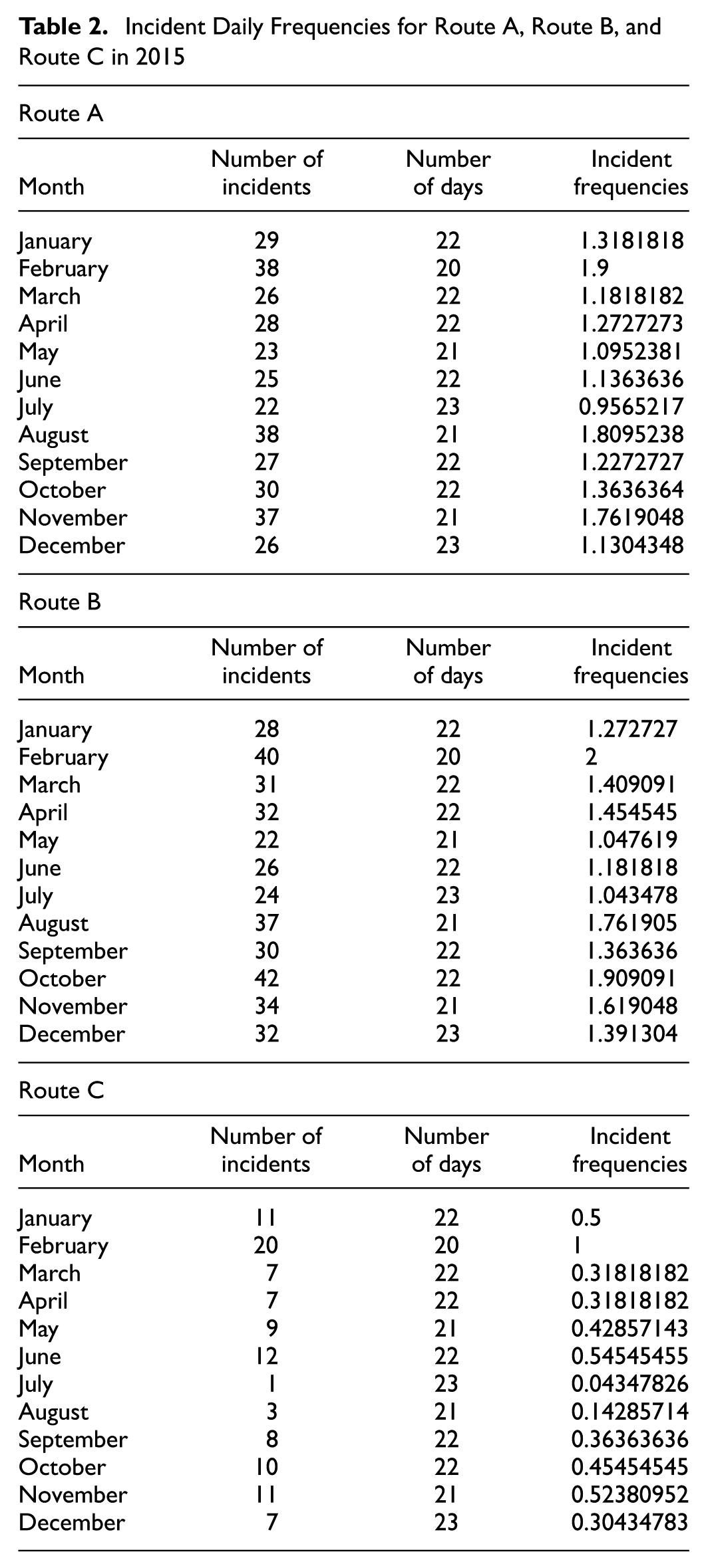
Incident Duration Statistics for Route A, Route B, and Route C

Route A
Incident type	Count	Average duration (min)	Std dev duration (min)	Max duration (min)	Min duration (min)	Percentage distribution (%)
1 Lane closed	14	25.1	17.4	52.4	8.2	22.2
2 Lane closed	3	60.4	58.3	123.5	8.7	4.8
3 Lane closed	0	0.0	0.0	0.0	0.0	0.0
Shoulder closed	46	63.1	32.8	136.9	11.7	73.0
Route B
Incident type	Count	Average duration (min)	Std dev duration (min)	Max duration (min)	Min duration (min)	Percentage distribution (%)
1 Lane closed	22	27.3	20.3	75.5	6.1	18.8
2 Lane closed	6	38.6	30.9	92.2	11.1	5.1
3 Lane closed	0	0.0	0.0	0.0	0.0	0.0
Shoulder closed	89	56.9	34.3	151.2	5.2	76.1
Route C
Incident type	Count	Average duration (min)	Std dev duration (min)	Max duration (min)	Min duration (min)	Percentage distribution (%)
1 Lane closed	8	171.5	182.6	540.0	28.5	17.0
2 Lane closed	0	0.0	0.0	0.0	0.0	0.0
Shoulder closed	39	49.9	24.0	108.7	6.1	83.0

Step 4: Calibrate Weather Probabilities

The HCM methodology also requires the specification of the probability of up to 11 different weather events by calendar month as input. Calibrating weather events requires historical weather data, which are used to estimate the probability, average duration, and standard deviation of duration of different weather events. In this paper, the research team used regional default weather event probabilities and default impacts. The HCM computational engine has a database of 10 years’ average of weather events probabilities for about a hundred largest metropolitan areas in the U.S., via the Weather Underground service ( 34 ). This study used the Raleigh-Durham Airport location to extract weather probabilities for the case studies.

Step 5: Validation

The results of the model were validated against travel times collected for the corresponding TMC segments on each route. As the HCM method uses 15-minute intervals as the basic temporal unit of analysis, 15-minute average reported TMC travel times were gathered from INRIX. These travel times were converted to a route TTI using a simultaneous path travel time estimation method ( 35 ). The TTI distribution of the HCM method was then validated against that counted from INRIX speed data.

Results

Key Reliability Performance Measures

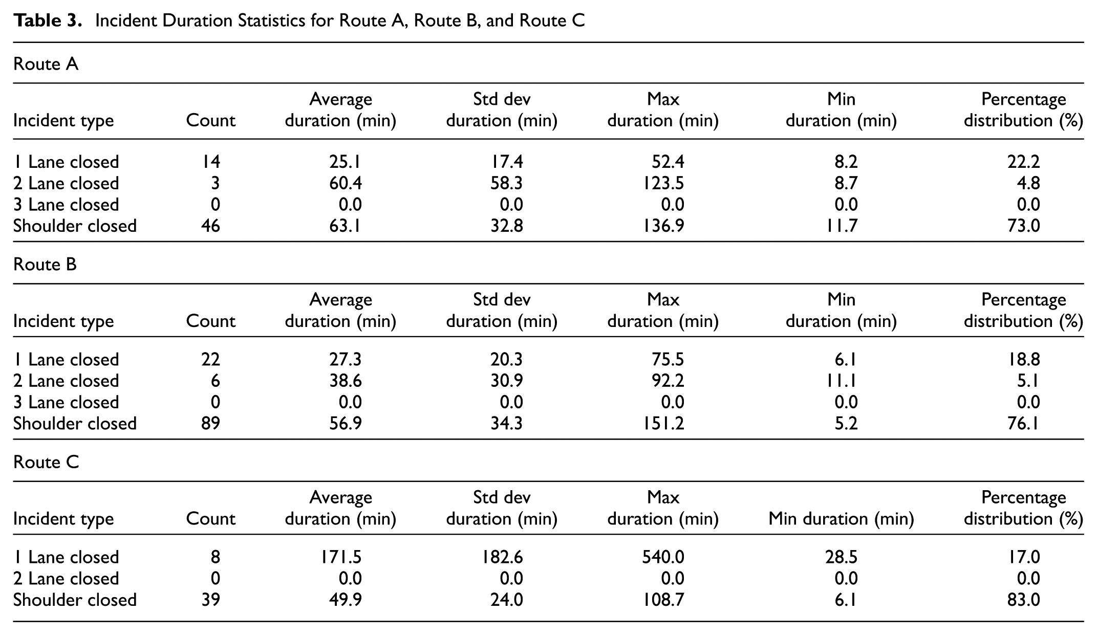
Figure 4 shows the various distribution statistics, alongside the cumulative distribution functions (CDFs) of the emerging TTI distribution estimated by the HCM reliability method and the empirical distribution of the INRIX travel times for the corresponding TMC set, for each of the 15-minute analysis periods over all weekdays in the year 2015. The average, 50^th percentile and 80^th percentile TTIs computed using the HCM method for all three routes were all within 15% of those reported by INRIX. FHWA has proposed new reliability performance measures, such as level of travel time reliability (LOTTR), as part of the Moving Ahead for Progress in the 21^st Century Act (MAP-21) ( 36 ). These metrics were calculated from the HCM method outputs and were found to be within 15% of INRIX observations. However, for Route A, the evening peak LOTTR values were significantly higher than observations from INRIX data. Similarly, the higher region of the distribution at or above the 90^th percentile TTI for Route A showed significant differences between the estimated and observed CDFs. For routes B and C, the overall CDFs and performance statistics were very consistent between the HCM method and empirical data. A two-sample Kolmogorov–Smirnoff (KS) test conducted on the three sets of CDFs, shown in Figure 4, showed that the distributions predicted by the HCM method were not significantly different from those observed from INRIX data at the 5% significance level. However, the two-sample KS test is not robust to difference in the tail end of distributions, which could be the reason it is unable to find differences between the CDFs in Figure 4a. The next section looks more closely at the incident scenario generation technique to investigate possible contributions to the large discrepancy in the upper regions of the TTI distribution for Route A.

Figure 4.

TTI reliability statistics and CDF from HCM and INRIX by route. (a) Route A; (b) Rote B; (c) Route C.

Discussion

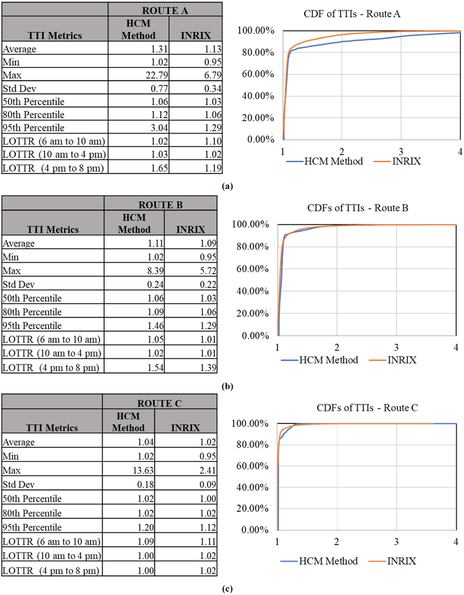
To further investigate the higher estimated TTIs at and above the 90^th percentile and the evening peak hour on Route A, incidents generated by the HCM method over time of day were compared with the TIMS log data. Figure 5 shows the total number of incident occurrence based on the HCM method, and in the incident logs, by hour of day. As shown in Figure 5a, the HCM model does not adequately capture the temporal incident trends found in the actual data (Figure 5b). This is primarily the result of the assumption in the HCM to use VMT distribution to allocate incident start time and location in the reliability scenarios. It is curious, however, that this pattern generated higher values of the 95^th percentile TTI in the HCM model, as was shown in Figure 4a. One possible explanation is that the accumulation of incidents starting in the early afternoon, based on the HCM model allocation, may have initiated congestion earlier, which was exacerbated as traffic demands kept increasing during the p.m. peak period.

Figure 5.

Incidents by time of day on Route A in (a) HCM method and (b) TIMS logs.

Another explanation of the discrepancy may be attributed to the discretization of all incident durations in the HCM model to the nearest 15 minutes. Hence, all actual incidents that clear in fewer than 15 minutes are not considered in the HCM approach. In effect, the method will tend to consistently model incidents with duration higher than empirical observations indicate. This pattern can be detected in Figure 6, which shows the incident duration distributions in both HCM and in TIMS. Finally, the HCM model does not consider any changes in traffic demand (i.e., as a result of diversions) in response to major incidents, which may also result in inflating their travel time effect when generating the TTI distribution.

Figure 6.

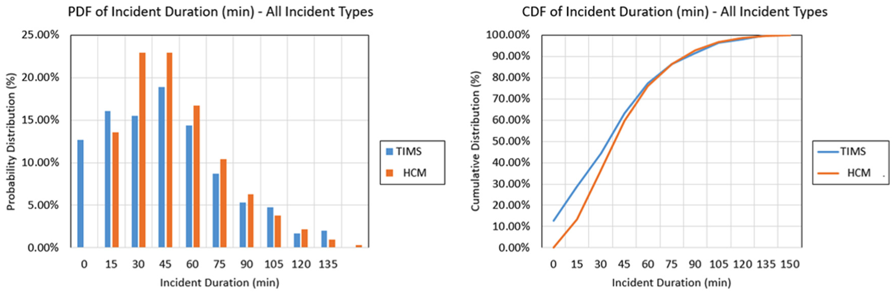
Distributions of incident duration: TIMS vs. HCM.

Conclusions and Future Work

This paper presented a case study implementation of the freeway reliability analysis procedure in the 6^th edition of the HCM. The major challenges involved in such implementation were identified and explained. The data needed for performing this analysis were explained and the results of the reliability analysis of the study sites were validated. The TTI distribution up to the 80^th percentile value was found to match closely those observed from probe-based travel times. However, the upper tail of the distribution from the HCM method yielded very high travel times. This can be explained by the fact that the HCM method models incidents with higher average duration than is seen in the empirical data, which exacerbates the poor travel conditions along the facility, especially when there are multiple incidents.

The incidents modeled in the HCM method follow the distribution of the VMT in a 24-hour period. However, for urban road segments, during peak periods, incidents can have a cascading effect as traffic demands increase when approaching the peak periods. The effect of one incident in a segment could lead to later secondary incidents on upstream segments. Further research is needed to investigate the probability of secondary incidents occurring on a facility as a direct effect of a downstream incident. With the use of mobile devices, drivers can choose to alternate routes more easily to avoid congestion caused by incidents. The HCM method does not take driver route choice or diversion into consideration when modeling the effect of incidents, thus probably inflating their effect. Lastly, the reliability scenario generation described in the HCM assumes that the effect of weather events and incidents are mutually independent. However, the input parameters for incident estimation in the model are not free from such an assumption. Future work is needed to incorporate the interaction of weather events and incidents on freeways for a more realistic modeling of reliability.

Footnotes

Acknowledgements

The research presented in this paper was funded by the NCDOT and FHWA through NCDOT project 2016-32 titled “SHRP2 Reliability Data and Analysis Tools: Implementation Assistance Program Pilot Study.” The research team is grateful for the support it has received from NCDOT and FHWA.

Author Contributions

The authors confirm contribution to the paper as follows: study conception and design: Nabaruna Karmakar, Seyedbehzad Aghdashi, Nagui M. Rouphail, Billy M. Williams; data collection: Nabaruna Karmakar, Seyedbehzad Aghdashi; analysis and interpretation of results: Nabaruna Karmakar, Seyedbehzad Aghdashi, Nagui M. Rouphail, Billy M. Williams; draft manuscript preparation: Nabaruna Karmakar, Seyedbehzad Aghdashi, Nagui M. Rouphail, Billy M. Williams. All authors reviewed the results and approved the final version of the manuscript.

The Standing Committee on Highway Capacity and Quality of Service (AHB40) peer-reviewed this paper (18-06088).

The views and opinions expressed in this paper do not necessarily reflect the views of the agencies, and no official endorsement should be inferred.

References

FHWA Office of Operations. Travel Time Reliability: Making It There on Time, All the Time. https://ops.fhwa.dot.gov/publications/tt_reliability/TTR_Report.htm. Accessed July 26, 2017.

Joseph

Traffic Jams Cost U.S. Drivers $1,200 a Year: Study. Reuters. 2017. https://www.usnews.com/news/us/articles/2017-02-20/traffic-jams-cost-us-drivers-1-200-a-year-study. Accessed July 27, 2017.

Federal Register 2016-08014. National Performance Management Measures; Assessing Performance of the National Highway System, Freight Movement on the Interstate System, and Congestion Mitigation and Air Quality Improvement Program. FHWA, U.S. Department of Transportation, Washington, D.C., 2016.

Highway Capacity Manual: A Guide for Multimodal Mobility Analysis, 6th ed. Transportation Research Board, Washington, D.C., 2016.

Aghdashi

Hajbabaie

Schroeder

B. J.

Trask

J. L.

Rouphail

N. M.

Generating Scenarios of Freeway Reliability Analysis: Hybrid Approach. Transportation Research Record: Journal of the Transportation Research Board, 2015. 2483: 148–159.

Tarnoff

Young

Crunkleton

Nezamuddin

, and University of Maryland. NCHRP 20-7, Task 202: Guide to Benchmarking Operations Performance Measures. Transportation Research Board of the National Academies, Washington, D.C., 2008.

Franklin

J. P.

Modeling Reliability as Expected Lateness: A Schedule-Based Approach for User Benefit Analysis, Royal Institute of Technology, Stockholm, Sweden. Proc., European Transport Conference, Noordwijkerhout, Netherlands, 2009.

Rakha

El-Shawarby

Arafeh

Trip Travel-Time Reliability: Issues and Proposed Solutions. Journal of Intelligent Transportation Systems, Vol. 14, No. 4, 2010, pp. 232–250. http://10.1080/15472450.2010.517477.

Cambridge Systematics, Texas A&M University, University of Washington, Dowling Associates, Street Smarts, Herb Levinson and Hesham Rakha. Analytical Procedures for Determining the Impacts of Reliability Mitigation Strategies. SHRP 2 Report S2-L03-RR-1. 2013. https://doi.org/10.17226/22806.

10.

Brilon

Geistefeldt

Zurlinden

Implementing the Concept of Reliability for Highway Capacity Analysis. Transportation Research Record: Journal of the Transportation Research Board, 2007. 2027: 1–8.

11.

Jia

Williams

Rouphail

Identification and Calibration of Site-Specific Stochastic Freeway Breakdown and Queue Discharge. Transportation Research Record: Journal of the Transportation Research Board, 2010. 2188: 148–155.

12.

Zhou

Rouphail

Analytical Models for Quantifying Travel Time Variability Based on Stochastic Capacity and Demand Distributions, Presented at 90th Annual Meeting of the Transportation Research Board, Washington, D.C., 2011.

13.

Kittleson and Associates. SHRP 2 Report S2-L08-RW-1: Incorporating Travel Time Reliability Analysis into Highway Capacity Manual. Transportation Research Board of the National Academies, Washington, D.C., 2013.

14.

Hajbabaie

Aghdashi

Rouphail

Enhanced Decision-Making Framework Using Reliability Concepts for Freeway Facilities. Journal of Transportation Engineering, Vol. 142, No. 4, 2016, p. 04016008. https://doi.org/10.1061/(asce)te.1943-5436.0000797.

15.

Al-Kaisy

A. F.

Hall

Guidelines for Estimating Freeway Capacity at Long-Term Reconstruction Zones. American Society of Civil Engineers: Journal of Transportation Engineering, Vol. 129, No. 5, 2002, pp. 572–577.

16.

Krammes

R. A.

Lopez

Updated Capacity Values for Short-Term Freeway Work Zone Lane Closures. Transportation Research Record: Journal of the Transportation Research Board, 1994. 1442: 49–56.

17.

Chitturi

Benekohal

Kaja-Mohideen

Methodology for Computing Delay and Users Costs in Work Zones. Transportation Research Record: Journal of the Transportation Research Board, 2008. 2055: 31–38.

18.

Schroeder

Rouphail

Corridor-Based Forecasts of Work-Zone Impacts for Freeways and Multilane Highways. Project HWY 10-08 Final Report. North Carolina Department of Transportation, Raleigh, NC, 2011.

19.

Aghdashi

Rouphail

N. M.

Hajbabaie

Schroeder

B. J.

Generic Speed–Flow Models for Basic Freeway Segments on General-Purpose and Managed Lanes in Undersaturated Flow Conditions. Transportation Research Record: Journal of the Transportation Research Board, 2015. 2483: 102–110.

20.

Chase

R. T.

Hajbabaie

Schroeder

B. J.

Incorporating Weather Effects in HCM Reliability Analysis. Presented at 92nd Annual Meeting of the Transportation Research Board, Washington D.C., 2013.

21.

Rakha

Farzaneh

Arafeh

Sterzin

Inclement Weather Impacts on Freeway Traffic Stream Behavior. Transportation Research Record: Journal of the Transportation Research Board, 2008. 2071: 8–18.

22.

Shi

Cheng

Jin

Ran

Chen

Effects of Rainfall and Environmental Factors on Traffic Flow Characteristics on Urban Freeway. Presented at 90th Annual Meeting of the Transportation Research Board, Washington, D.C., 2011.

23.

Dehman

Effect of Inclement Weather on Two Capacity Flows at Recurring Freeway Bottlenecks. Transportation Research Record: Journal of the Transportation Research Board, 2012. 2286: 84–93.

24.

Aghdashi

Rouphail

Hajbabaie

Estimation of Incident Propensity for Reliability Analysis in the Highway Capacity Manual. Transportation Research Record: Journal of the Transportation Research Board, 2013. 2395: 123–131.

25.

Skabardonis

Petty

K. F.

Bertini

R. L.

P. P. Varaiya

N. H

Rydzewski

The I-880 Field Experiment: Analysis of the Incident Data. Transportation Research Record: Journal of the Transportation Research Board, 1997. 1603: 72–79.

26.

Schroeder

Rouphail

Aghdashi

Deterministic Framework and Methodology for Evaluating Travel Time Reliability on Freeway Facilities. Transportation Research Record: Journal of the Transportation Research Board, 2013. 2396: 61–70.

27.

Williges

McCullough

Chu

Amatya

Kuo

Lin

Chu

SHRP 2 Reliability Project L38A: Pilot Testing of SHRP 2 Reliability Data and Analytical Products: Southern California. Transportation Research Board of the National Academies, Washington, D.C., 2014.

28.

Sobolewski

Polum

Morris

Loos

Anderson

SHRP 2 Reliability Project L38B: Pilot Testing of SHRP 2 Reliability Data and Analytical Products: Minnesota. Transportation Research Board of the National Academies, Washington, D.C., 2014.

29.

Hadi

M.Y. Xiao

Wang

Jia

Edelstein

Lopez

SHRP 2 Report: Pilot Testing of SHRP 2 Reliability Data and Analytical Products: Florida Pilot Site. Transportation Research Board of the National Academies, Washington, D.C., 2014.

30.

Nisbet

Bremmer

Yan

Murshed

Wang

Zou

Zhu

Dunlap

Wright

Zhu

Zhang

SHRP 2 Reliability Project L38D: Pilot Test of SHRP 2 Reliability Data and Analytical Products: Washington. Transportation Research Board of the National Academies, Washington, D.C., 2014.

31.

Trask

J. L.

Seyedbehzad

John

Nagui

M. R.

Capacity Calibration for Freeway Facilities Methodology in the HCM: A Metaheuristic Approach. Presented at 96th Annual Meeting of the Transportation Research Board, Washington D.C., 2017.

32.

RITIS. Regional Integrated Transportation Information System. 2016. www.ritis.org.

33.

Webmaster. Traveler Information Management System. NCDOT. https://tims.ncdot.gov/tims/. Accessed July 31, 2017.

34.

Weather Underground. https://www.wunderground.com. Accessed July 31, 2017.

35.

Chase

R. T.

Williams

Rouphail

Kim

Reporting Path Travel Times for ATIS Reliability. Presented at the INSTR 2012 Conference in Hong Kong, China, 2012.

36.

MAP-21 Proposed Measures for Congestion, Reliability, and Freight: Step-by-Step Calculation Procedures. FHWA, 2016. https://www.apta.com/gap/fedreg/Documents/MAP-21_Proposed_Measures_for_Congestion%2C_Reliability%2C_and_Freight.pdf.