
Abstract
This study demonstrates three methods for uncertainty propagation in transportation and land-use models (LUMs): Local Sensitivity Analysis with Interaction (LSAI), Monte Carlo (MC), and Bayesian Melding (BM). Two case-study settings are used to illustrate how these methods work, allowing for inter-method comparisons. LSAI can provide the sign of change implied by changes in model inputs, the relative importance of changes in different inputs, and a decomposition of changes in outputs due to the impact of inputs’ individual and interactive. LSAI is limited to relatively small-size problems because its computing time rises exponentially with the number of (groups of) inputs. Moreover, LSAI obtains only point estimates, while MC and BM methods can deliver entire distributions of each output through an understanding of the uncertainty in all model inputs and parameters. MC delivers each output’s distribution and requires hundreds of samples, especially for more accurate results. Fortunately, MC methods are especially useful for high-dimensional problems because convergence rates are not a function of model dimensionality and errors depend only on sample size and input uncertainties. BM delivers posterior distributions for model outputs, using prior probability distributions and likelihoods of inputs and parameters, along with validation of/comparison to intermediate model outputs. A BM approach can be extremely expensive, in terms of computing time, since it requires several hundred model runs.
Scientific computing involves large-scale simulations to represent real-world phenomena, like the evolution of cities and their traffic patterns. With improvements in computing capabilities and more efficient algorithms, results can be more accurately simulated to represent real-world conditions. Models allow for accurate forecasts over longer prediction periods. Predictions are typically affected by uncertainties in input data and model parameters, and by incomplete knowledge of underlying behaviors ( 1 ). Models (and the systems they represent) are often explicitly stochastic ( 2 ), with random components being generated and used throughout the predictive process. It is very important for system design optimization and policy-making to capture and represent this uncertainty information appropriately in model results. Much work has been done in land-use forecasting (3–5).
Few studies have begun to examine uncertainty propagation in the context of the integrated land-use transportation modeling framework because of the required integration of metropolitan and statewide transportation plans with land-use plans by the Intermodal Surface Transportation Efficiency Act (ISTEA) of 1991 ( 6 ).
Obviously, one must first identify sources of uncertainty ( 7 , 8 ), to carry out a probabilistic analysis of a system. Pradhan and Kockelman ( 3 ) reviewed the literature on the sources of uncertainty in land-use transportation models. Later, Sevcikova et al. ( 9 ) reviewed the key sources of uncertainty for UrbanSim land-use modeling outputs.
Uncertainty quantification is the process of representing imperfectly known or understood inputs and parameters, propagating this variability through the model system and then characterizing the uncertainty in the model’s results. The outcome usually comes with attached “error bars” to indicate uncertainty ranges. Generally, the uncertainty is usually represented by interval mathematics ( 10 ), fuzzy theory ( 11 ), and probabilistic analysis ( 8 ). In the probabilistic analysis approach, uncertainties described by probability distributions are associated with model inputs to estimate the outputs’ probability distributions by using UrbanSim ( 3 ). However, the methods to research uncertainty propagation in the integrated land-use transportation modeling framework still attract attentions.
This work demonstrates and compares methods for uncertainty propagation in complex transportation and land-use models (LUMs). The following sections provide a literature review, introduction and two test examples for uncertainty propagation in transportation and LUMs, along with a summary of findings.
Literature Review
Many researchers have examined different methods for anticipating and understanding output uncertainties. This paper introduces three methods for forecasting uncertainty in land-use and transportation model outputs: Local Sensitivity Analysis with Interaction (LSAI), Monte Carlo (MC) method, and Bayesian Melding (BM) method. Two reasonably transparent transportation settings are then used to illustrate and review these methods.
LSAI
Sensitivity analysis is the study of how uncertainty in the output of a mathematical model or system (numerical or otherwise) can be apportioned to different sources of uncertainty in its inputs ( 12 ). There are many different ways of conducting sensitivity analyses; however, the various analyses may not produce identical results in answering these question. Thus, Hamby ( 13 ) summarized many available methods to conduct sensitivity analyses by presenting details of the types of sensitivity analyses utilized for various modeling situations. Hamby ( 14 ) compared the assessment of several methods and intended to demonstrate calculation rigor and parameter sensitivity rankings resulting from various sensitivity analysis techniques.
Local sensitivity analysis is the assessment of the local impact of inputs’ variation on the model response by concentrating on the sensitivity in the vicinity of a set of input values. Such sensitivity is often evaluated through gradients or partial derivatives of the output functions at these inputs, so other inputs’ values are held constant when studying the local sensitivity of a specific input. Kockelman ( 15 ) ran a gravity-based land-use model (G-LUM) over three alternative scenarios, with total employment counts (EMP), household counts (HH) and link impedances or travel times (TT) increasing by 50%, utilizing each set individually.
To overcome the limitations of local methods, Saltelli et al. ( 12 ) used the global sensitivity analysis in contrast to local sensitivity analysis to consider the entire range of input variations.
Besides the joint sensitivity of generic model outputs for small changes in all inputs (including parameters) addressed in ( 16 , 17 ), Saltelli and Tarantola ( 18 ) defined group sensitivity indices in the context of a global sensitivity analysis. As far as finite changes are concerned, Borgonovo ( 19 ) introduced sensitivity measures for individual exogenous variables. To find sensitivity measures for specific input factor sets (typically, sets of parameters), Borgonovo and Peccati ( 20 ) proved that a change in model output is decomposed as a function of factors with the same structure as the parameter decomposition and introduced factor finite-change sensitivity indices (FCSI) for model parameters to investigate the relationship between the factor FCSIs and parameter FCSIs. Then, Borgonovo et al. ( 21 ) used the G-LUM by Kockelman ( 15 ) to illustrate LSAI techniques and found that the outputs respond almost additively to variations in model inputs over the given scenarios. Wang and Kockelman ( 22 ) applied LSAI to evaluate random–utility-based multiregional input-output models by producing FCSI for the variation of inputs under different scenarios.
MC Method
MC techniques have been widely used for uncertainty propagation due to their conceptual simplicity and ease of implementation. In MC techniques, one samples random variables, runs an ensemble of simulations, and simply presents the distribution of outputs, for all uncertainty statistics. A reasonable result usually requires many ensemble runs, which is computationally expensive for large-scale systems. More efficient approaches need to be developed to represent and propagate uncertainties in large-scale simulations ( 23 ).
Zhao and Kockelman ( 24 ) conducted a study of the propagation of uncertainty in four-step travel demand models by using MC simulation to quantify variability in model outputs. Krishnamurthy and Kockelman ( 25 ) researched propagation of uncertainty in transportation LUMs through multivariate MC sampling of 200 scenarios. Harvey and Deakin ( 26 ) conducted a similar study to consider uncertainty in population growth, fuel price and household income levels in the Los Angeles region. Thompson et al. ( 27 ) examined the impact of higher-than-projected population estimates on emission trends for metropolitan regions in California. Saadi et al. ( 28 ) integrated Markov Chain MC simulation and profiling-based methods to capture the behavioral complexity and the great heterogeneity of agents of the true population for large-scale microsimulation scenarios of transportation and urban systems. Clay and Johnston ( 29 ) aimed to research which sources of uncertainty have the largest impact on outputs in a fully integrated land-use and transportation forecasting models. They ran all possible combinations of each variable at each level of uncertainty to analyze the impacts of uncertainty on the model’s outputs. Clay et al. ( 30 ) used point-estimate inputs to research how uncertainty affects the Large Zone Economic Module outputs by tracking the effects of this uncertainty through the various submodels to the model outputs.
BM Method
Pradhan and Kockelman ( 3 ) examined the propagation of uncertainty in the context of UrbanSim. However, this study analyzed only the sensitivity to a small sample of selected input values and explored the effect of these changes on outputs, in addition to simple stochastic simulation error from variation in random seeds.
Another approach to extrapolate prediction accuracy for LUMs was taken in ( 31 ). Models calibrated at different time points were used to simulate the present land-cover change and estimate how accurately the model will predict the future through a measure derived by a validation with empirical data. Sevcikova et al. ( 9 ) developed and then applied BM by extending an earlier method to agent-based stochastic models for calibrating a stochastic model system with respect to uncertainty. This method encodes all available information about model inputs and outputs in terms of prior probability distributions and likelihoods, and used Bayes’ theorem to obtain a posterior distribution for any quantity. However, BM can be very computationally intensive since it requires several hundred runs of the model. Thus, they provided various ways to reduce the required time ( 9 ). Based on work ( 9 , 32 ), Sevcikova et al. ( 2 ) described the first incorporation of uncertainty assessment into the development of an official land-use forecast published by a metropolitan planning organization. They demonstrated how BM for assessing uncertainty could be used to support the application of an academically founded land-use model.
Introduction to Three Methods
Introduction to LSAI
Mathematical models are used to denote input-output mappings as follows:

where
Therefore, the base-case output of the simulation

Then,
where
and where

where
For the
According to

where
As discussed in the literature (
18
,
33
), the sign of the first-order indices
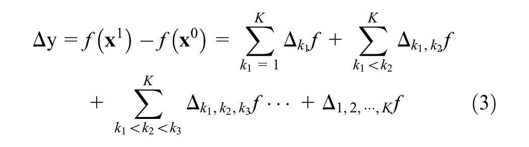
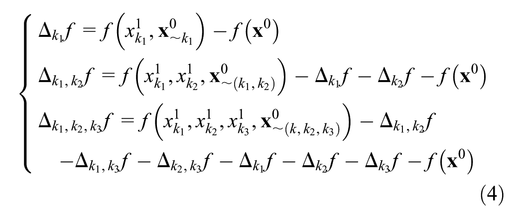
All FCSI can be computed by use of 2
K
simulations if there are K (or group of) exogenous variables whose variations are of interest. The triplet
Introduction to MC Methods
The MC method is a broad class of computational algorithms that rely on repeated random sampling to obtain numerical results. MC is useful for simulating phenomena with significant uncertainty in inputs and systems with many coupled degrees of freedom (
34
,
35
), especially for high-dimensional problems because the convergence and convergence rate are not concerned with the dimensions of the problems. The error of MC is defined by
Introduction to BM Method
Sevcikova et al. (
2
) presented a figure to show the basic concept of BM developed for deterministic models. There is a prior distribution of model inputs
The primary BM stages or steps are as follows ( 9 ):
Draw a sample {
For each
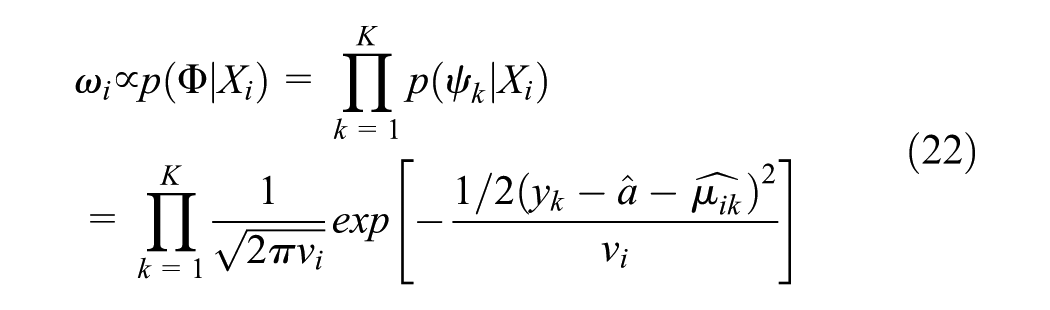
Compute weights
The posterior distribution of

In Equation 7, the conditional distribution

Two Test Examples
To illustrate these different methods for uncertainty propagation in transportation and LUMs, Example 1 offers LSAI and MC applications and Example 2 offers a BM application.
Example 1. Figure 1’s small test network enables application of a simple travel demand model (TDM), with three nodes (with node 1 as the origin, and 2 and 3 as destinations) and four links. (*,*) denotes the free-flow travel time and capacity on each link.
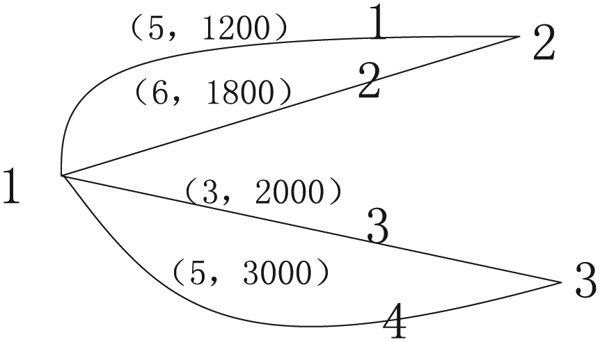
The test network.
This TDM’s equations are as follows:


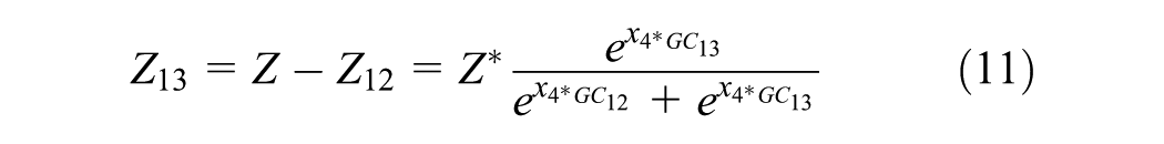


where Z denotes number of trips generated, Z1j denotes number of trips going from origin node 1 to destination node j (j = 2, 3), GC1j denotes generalized cost going from node 1 to destination nodes j (j = 2,3), and LCi denotes generalized cost of using link i (i=1,2,3,4). This assumes the travelers have the same value of time (VOT), which is
Equation 9 describes trip generation per zone, and Equations 10 and 11 describe trip distribution. There is no mode split because only one mode is used in this example. Route choice is obtained via traffic assignment based to the network, assuming shortest-path user equilibrium ( 37 ) and feedback of chosen routes and TT to trip distribution.
The Bureau of Public Roads (BPR) function is used here for TT on each link i, with
LSAI for Example 1
LSAI is applied on the test example by increasing all inputs by 10%. The change of each model’s outputs (traffic flow on links) from

The ith-order indices as well as their sum and the total-order indices using LSAI: (a) first-order indices; (b) second-order indices; (c) third-order indices; (d) fourth-order indices; (e) sum of ith-order indices; (f) total-order indices; (g) effect of interactions associated with inputs.
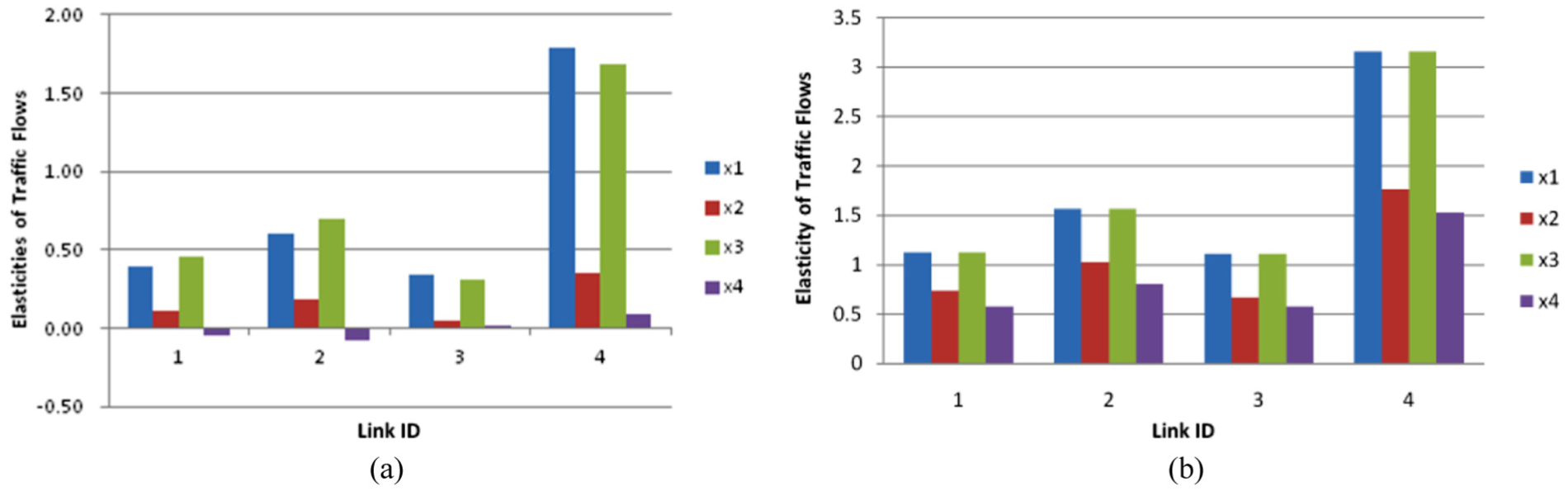
Elasticity of first-order and total-order indices of link flows using LSAI: (a): elasticity of first-order index; (b): the elasticity of total-order index.
Figure 2a shows that increasing inputs
Figure 2c shows that almost all third-order indices deliver negative effects on all links’ traffic flows with the exception of third-order interactions among
Figure 2d shows how the fourth-order index has positive effects on all links, with its largest effect on link 4’s traffic flow and its smallest effect on the traffic flow of links 1 and 3. Figure 2e shows that the sum of the third-order index has non-positive effects on all links (zero for link 1, negative for other links). The sums of other order indices positively affect all links. Among all sums of the order indices with positive effects on all links, the sum of the fourth-order has the biggest effect on the traffic flow on links 1, 2, and 3, while the sum of the first-order has the biggest effect on the traffic flow on link 4. Figure 2f shows that the total-order indices positively affect all links. Inputs
Figure 2g shows the effect of interactions associated with
Finally, Figure 3 provides elasticities of first-order and total-order indices. They have the same trend with the first-order index and the total-order index in Figure 2a and f , which resulted from the same increasing of inputs of this test example.
MC for Example 1
MC was applied with the test example by randomly generating 16 different sets of model inputs and parameter values, and then solving the TDM for its equilibrium. In general, the number of simulation runs needs to be large enough to obtain robust and accurate results. Here, 16 different sets of inputs were randomly chosen, using the Example 1 distributions described earlier (for x1 through x4). Final link flows were obtained from the converged user equilibrium (UE) assignment results. The mean, SD and CoV for four links’ traffic flows are computed as follows: Link 1’s mean (veh/day), SD and CoV values are 1006, 58.83 and 0.0584. Link 2’s mean (veh/day), SD and CoV values are 1279, 165.6 and 0.1294. Link 3’s mean (veh/day), SD and CoV values are 1569, 21.87 and 0.0139. Link 4’s mean (veh/day), SD and CoV values are 1307, 386.4 and 0.2957.
The CoVs of link 2 and 4 traffic flows are larger than the inputs’ starting CoV values (of 0.10), suggesting that final flow uncertainties/variations can be compounded and end higher than input uncertainties. CoV values for link 1 and 3 flows are smaller than 0.06, which is lower than any inputs’ uncertainty (as measured using CoV, or SD/mean). Moreover, the ratios of traffic flow versus capacity (v/c ratios) on links 1 through 4 are computed to be 0.84, 0.71, 0.78 and 0.44, respectively. The flow uncertainty appears not to have a strong relation with congestion, which is consistent with the result in ( 24 ).
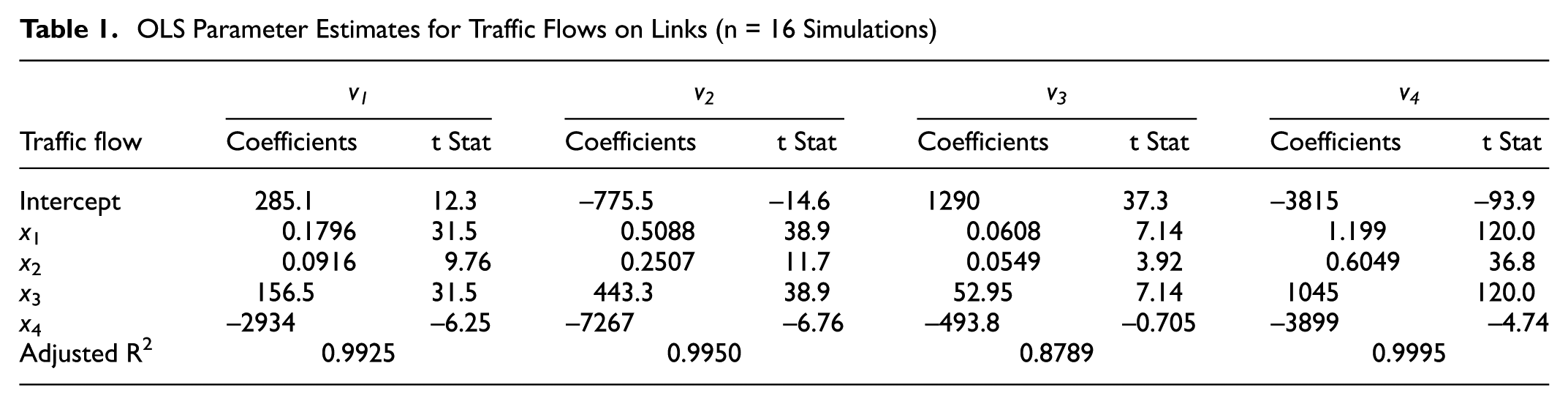
For better understanding and interpretation of the results, ordinary least squares (OLS) regression was used to identify model inputs that are key contributors to uncertainty in model output (Table 1), assuming simple linear relationships between inputs (or combinations and transformations of model inputs, if one desires) and outputs. Only 16 input samples were used here, yet t-statistics and R2 values are very high in this toy network, as shown in Table 1.
OLS Parameter Estimates for Traffic Flows on Links (n = 16 Simulations)
BM for Example 2
Example 2. To illustrate how BM works, an integrated land-use and transportation model is presented, based on the following model equations:
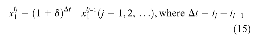


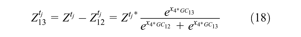


where
In this Example 2, Equation 15 is a simple LUM, while Equations 16–21 describe a simple TDM. The LUM reacts to travel network changes, and vice versa. However, the link from TDM to LUM is not as strong as the link from LUM to TDM because it is difficult to move one’s home (and/or business) and costly to construct new buildings. Thus, here we investigate only the forward effect of land-use changes on the TDM outputs, rather than allow a feeding back of TDM outputs to LUM decisions. In other words, TT from the TDM’s traffic assignment step feed forward into the subsequent year’s LUM equation.
Here, 16 samples of random input values were chosen, and the model was run three times for each set of inputs (including all uncertain parameters). Therefore, I = 16, J = 3, and K = 4. Starting back in year t0 = 2010, t1 = 2015 served as the “present” year (for output validation, or comparisons to measured/regionally observed values), and t2 = 2020 served as the final prediction year. According to BM,
where
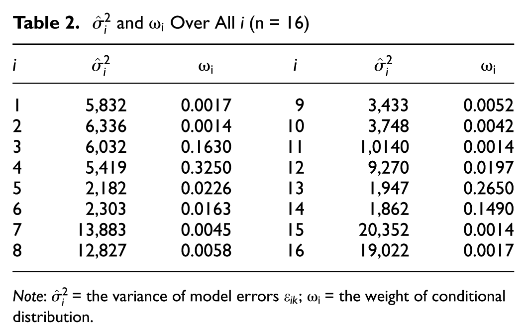
Note:
Posterior distributions of link-level traffic flows (Yk values) are given by a mixture of normal distributions, as follows:
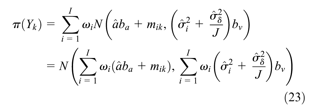
where
Therefore, link k’s traffic flow outputs will follow normal distribution:
In this way BM methods can provide model outputs (future-year predictions) by using present-year inputs. BM assesses output uncertainties for a land-use transport model by combining all available information on model inputs and outputs in a Bayesian way, to provide a posterior distribution of outputs.
Conclusion
In this paper, two small travel demand modeling examples (one with a land-use equation) were used to demonstrate how LSAI, MC, and BM methods of uncertainty characterization function and to illuminate their strengths and weaknesses. LSAI can provide the sign of change implied by the changes of inputs, the relative importance of change of inputs and the decomposition of change of output into the individual and interaction changes of inputs. Although LSAI needs just about 2 ×K simulations to obtain first-order impact indices, a model’s total-order indices and interactive effects associated with K (groups of) inputs require 2 K simulations, thus rising exponentially in respect to the number of exogenous (input) variables, to obtain the individual effects and all interaction effects.
Thus, LSAI will be effective only for problems with a small number of exogenous variables because it needs thousands of simulations for models with more than 10 inputs. Moreover, LSAI provides only point estimates, while MC and BM methods can provide distributions of needed outputs. MC involves random sampling of the distribution of inputs and successive model runs until obtaining a statistically significant distribution of outputs. MC can be used to solve problems with probability structures or non-probabilistic problems (such as finding the area under a curve), and can be used with time-series models (like land-use and travel changes, forward in time) or one-time-point models, where no validation data are needed. It is straightforward to obtain output distributions via MC random sampling of the distribution of inputs and parameters. However, such activities require hundreds of samples, even for small scale problems, to obtain accurate results. MC is especially useful for high-dimensional problems because its convergence and convergence rate do not depend on the problem’s dimensionality and prediction errors depend only on the number of samples and the standard deviations of inputs.
While LSAI can only address deterministic problems, MC and BM methods are useful in solving both deterministic and stochastic problems. BM is a way of putting analysis of simulation models on a solid statistical basis. Its advantage is that it can obtain the posterior distribution of all model outputs from prior probability distributions and likelihoods of all model inputs (which include model parameters). Users are provided with probability intervals around forecasts with calibrated uncertainty statements, which add value to model validation, scenario comparison and external review and comment procedures. However, BM can be extremely computationally expensive, since it requires several hundred runs of the model. Moreover, intermediate outputs must also be known for intermediate validation. As a result, MC appears to be the best way for complex system modelers and planners to anticipate uncertainty in our urban systems’ futures.
Footnotes
Acknowledgements
This paper was financially supported by the National Natural Science Foundation of China (71471167). The authors of this paper wish to thank Scott Schauer-West for his editing and administrative support, and several anonymous reviewers for their helpful suggestions.
Author Contributions
The authors confirm paper contributions as follows: study conception and design: KK and GW; data collection/model specifications: GW; analysis and interpretation of results: KK and GW; draft manuscript preparation: GW. All authors reviewed the results and approved the final version of the manuscript.
The Standing Committee on Transportation Demand Forecasting (ADB40) peer-reviewed this paper (18-00488).