Development of a Hot Mix Asphalt Location Cost Index for the Alabama Department of Transportation

Abstract

Asphalt is one of the most critical commodities for the U.S. infrastructure. It is used as a paving material on the majority of roadways across the country. In Alabama, this material is used in approximately 98% of all paved roads, consuming about 40% of the Alabama Department of Transportation (ALDOT) annual construction budget. Because of the considerable importance of this material, any improvements in ALDOT’s hot mix asphalt (HMA) cost-estimating procedures are expected to be reflected in better budget control and a more effective use of ALDOT’s limited available resources. This paper presents a HMA Location Cost Index (LCI) intended to contribute to ALDOT’s efforts toward the improvement of its cost-estimating practices. This is an annual LCI aimed to quantify changes in HMA prices among three geographic regions in Alabama: north, central, and south regions. The development of the LCI involved the use of advanced data collection, cleaning, and processing techniques to analyze historical bid data from 3661 projects awarded by ALDOT between 2006 and 2016. The potential contribution of the proposed LCI to improving ALDOT’s current cost-estimating system is demonstrated via statistical significance testing and through the application of an innovative moving-window cross-validation algorithm previously developed by the authors.

After almost 150 years of history in the U.S., asphalt paving has become a mature method and a key player in socio-economic growth and development. Asphalt is currently the most popular form of road surfacing in the U.S., with about 94% of all paved roads and highways surfaced with this material ( 1 ). The National Asphalt Pavement Association estimates that there are about 3,500 asphalt plants across the country, producing about 400 million tons of asphalt every year, worth over $30 billion. A large portion of this production is used by state transportation agencies (STAs) to expand, maintain, and repair the national highway system. Asphalt paving activities consume the most part of STAs’ available funding ( 2 ). Therefore, it is critical for these agencies to have accurate and reliable cost-estimating systems for this type of project.

The main challenge faced by STAs in their efforts to produce effective cost estimates is associated with their capacity to identify, understand, and model the impacts of the main cost-influencing factors on transportation construction projects. This paper briefly describes some of the most relevant cost-influencing factors; however, it is mainly focused on assisting the Alabama Department of Transportation (ALDOT) with the incorporation of one of these factors into the cost-estimating process for asphalt paving projects. The cost-influencing factor addressed in this paper is geographic location.

The paper presents the development and validation of a Hot Mixed Asphalt (HMA) Location Cost Index (LCI). This is an annual LCI aimed to compare HMA prices across three different regions in Alabama (north, central, and south) and to adjust asphalt unit prices according to the geographic location of each project. The index was developed using historical bid data provided by ALDOT. Although the final LCI presented in this paper was built with 6 years of bid data (from 2011 to 2016), a considerable part of the data analysis was conducted over an 11-year period of time on bid data from 3661 projects awarded by ALDOT between 2006 and 2016. The LCI was developed with the most recent 6 years of data in an attempt to demonstrate the effectiveness of the proposed methodology under current market conditions. Statistical testing revealed apparent significant changes in the asphalt market around 2010, leading the authors to assume that the use of more than 6 years of data could result in the use of projects executed under different market conditions.

The HMA-LCI presented in the paper was actually developed to compare unit prices across the state of Alabama for a single case study item. This is the HMA pay item most commonly used in ALDOT’s construction contracts: “Superpave Bituminous Concrete Wearing Surface Layer, 1/2” Maximum Aggregate Size Mix – Item ID 424A360.” Unit prices for the case study item are estimated on a tonnage basis and included “all materials, procurement, handling, hauling, and processing cost, and includes all equipment, tools, labor, and incidentals required to complete the work” ( 3 ). Although the considerable relevance of the case study item suggests that it could be a suitable proxy for the overall price of purchasing and placing HMA, ALDOT should consider the development of separate LCI for other frequently used HMA pay items, by replicating the process described throughout this paper.

The potential contribution of the proposed LCI to improving ALDOT’s current cost-estimating system is demonstrated through the application of an innovative moving-window cross-validation (MWCV) algorithm previously developed by the authors ( 4 ). Measures for estimating accuracy and reliability were obtained through the MWCV algorithm before and after incorporating the location factor into the cost-estimating process. The comparison of the “before” and “after” cost-estimating performances, via statistical significance testing, revealed that the proposed HMA-LCI has the potential to significantly improve cost-estimating effectiveness for the case study item.

Hot Mix Asphalt in the State of Alabama

“Roadways form the backbone of Alabama’s economy by getting residents to work, transferring goods and services to market, and connecting residents and visitors to recreational and tourist destinations” ( 5 ). The state of Alabama has over 102,000 miles of public roads, including 11,000 miles maintained by ALDOT ( 5 ). Approximately 98% of all paved roads in Alabama are surfaced with asphalt ( 6 ). Asphalt paving is the most common type of work done by ALDOT. On average, the annual amount paid by ALDOT for HMA between 2012 and 2016 corresponds to over 40% of its annual construction budget. This percentage refers to “superpave bituminous concrete base, binder, and wearing surface layers,” defined under Section 424 of ALDOT 2018 Standard Specifications for Highway Constructions ( 3 ) as “a hot or warm bituminous plant mixed pavement layer placed on a prepared surface” ( 3 ).

Importance of Effective Construction Cost Estimating

In project management, a project is defined as a “temporary endeavor undertaken to create a unique product, service, or result” ( 7 ), and these endeavors usually demand the consumption of different types of resources (i.e., money, time, materials, and labor/equipment hours). Under this definition, cost estimating is the process to predict the approximate amount of money required to complete a project. The final amount depends on the required quantities for the other resources. Higher costs are expected from larger projects that require a significant consumption of materials and labor/equipment hours. Cost-estimating processes are used in all industries and businesses, not only on construction projects. However, unlike other industries, a single construction owner or contractor may need to manage a highly diversified project portfolio in terms of project-specific scopes, designs, and requirements. Each construction project is characterized by a unique combination of several factors, including project objectives, deliverables, location, environmental requirements, technical complexity, and so forth. This uniqueness, and the fact that it is virtually impossible to accurately quantify the impact of all these factors on a project, makes construction cost estimating a particularly challenging process.

From an owner’s perspective, cost estimates are commonly used to determine whether or not a project should proceed and to allocate the required funds for its completion ( 8 ). On the other hand, a construction contractor uses cost estimates to assess its financial capacity to undertake a given project and to prepare the bid for an owner. In both cases, cost estimates are basically used for risk assessment purposes, to support business decisions, and to maximize returns from project portfolios. Therefore, effective cost estimating could be translated into more effective decision-making and greater returns for owners or contractors ( 9 – 11 ), which would justify research efforts as those presented in this paper, aimed to assist STAs with the improvement of their cost-estimating efforts.

Cost-Estimating Effectiveness

There are several internal and external factors affecting the accuracy of construction cost estimates and it is virtually impossible to identify all of them, as well as to exactly quantify their impacts on estimating accuracy. Thus, effective cost estimating should not be conditioned to a 100% accuracy, as that would be unrealistic. Effective cost estimating is defined in this study as the capacity of STAs to maximize estimating accuracy and reliability. Accuracy refers to the level of validity of the system, which is the degree to which the system truly measured what it is intended to measure ( 12 ). Accuracy is usually assessed with measures of central tendency such as mean, median, and mode values. In this study, the level of accuracy for a given HMA price estimate is determined by the absolute percentage error (APE), as shown in Equation 1; the overall accuracy of the system is determined by averaging the APEs of all projects on which the system was applied during the validation process. This is called the mean absolute percentage error (MAPE) and is calculated as shown in Equation 2. MAPE values are commonly used to measure and compare accuracy between cost-estimating models ( 13 ).

A P E = \frac{| A_{i} - E_{i} |}{A_{i}} \times 100 %

(1)

M A P E = \frac{\sum_{i = 1}^{n} \frac{| A_{i} - E_{i} |}{A_{i}}}{n} \times 100 %

(2)

where: APE = Absolute Percentage Error

MAPE = Mean Absolute Percentage Error

A_i = Actual unit price for HMA in project i

E_i = Estimated unit price for HMA in project i

n = Number of projects using HMA during period under consideration for validation

On the other hand, estimating reliability refers to the degree of consistency in the outputs of quantitative models ( 12 ). Under the context of this study, and using the terms introduced in the previous paragraph, reliability is the degree to which the proposed cost-estimating system consistently yields similar APEs every time that it is used. Thus, reliability is measured in terms of variance and standard deviation values, which indicate the level of dispersion of the APEs produced by the system.

Cost-Influencing Factors in the Construction Industry

This paper corresponds to the second phase of a larger research initiative intended to improve ALDOT’s cost-estimating practices, an initiative that started with a comprehensive literature review to identify the main factors affecting cost-estimating effectiveness in the construction industry. Project scale, time, geographic location, level of competition, and estimating uncertainty have been identified by the ASCE ( 14 ) as major cost-influencing factors. The first two factors (scale and time) have already been addressed during the previous research phase ( 4 ), and this paper is focused on assessing the cost impact associated with project location (the third factor). Future research efforts will be directed to analyze the last two factors (level of competition and estimating uncertainty). The five cost-driven factors are described below:

The influence of project scale on construction costs is associated with the concept of economies of scale. According to this concept, lower unit prices should be expected from larger quantities of work given that fixed costs can be distributed among a greater number of pay item units ( 15 – 17 ). The authors have previously modeled the quantity–unit price relationship non-linear regression equations at the pay item level ( 4 ).

The time factor is associated with the constant fluctuations of construction prices over time. The total cost of a given project today is not expected to be equal to the cost of the same project a year ago or next year. When previously addressed by the authors ( 4 ), the analysis of the time factor was used to answer two questions that that arise when data from old projects are used to produce cost estimates for current or future projects:

How much historical data should be used in cost intimating?

How can old prices be adjusted to reflect current construction market conditions?

The first question was answered through a systematic implementation of the same MWCV algorithm used in this paper, and the second question was addressed by proposing the use of a cost index to counteract the effects of time on data-driven cost estimating.

The location factor refers to the fact that different geographic conditions bring different types challenges and project requirements. Therefore, different prices could be expected for the same type of work or commodity at different locations. The existing literature has attributed the price variability between geographic locations to several factors, such as local climate and geological conditions; availability of qualified local labor, suppliers, and subcontractors; and local applicable regulations ( 18 – 20 ). Traffic characteristics at the jobsite are also a key factor to be considered when estimating costs for transportation construction projects, as these dictate the strictness or laxity of traffic control requirements, increasing or reducing construction costs ( 21 ). This factor is addressed in this paper with the proposed LCI.

Level of competition refers to the degree of competitive pressure perceive by bidders. An anticipated large number of contractors competing on a given project or the anticipated participation of a strong bidder could increase the perceived level of competition, forcing contractors to reduce their profits to ensure the submission of competitive price proposals ( 22 ).

The last factor refers to the unavoidable estimating uncertainty inherent in construction cost estimating. This factor will be assessed by the authors in future research via probabilistic analysis to convert traditional deterministic estimates into risk-based cost estimates. A risk-based estimate is a probability distribution function that contains all possible construction cost values with their respective probability of occurrence ( 8 ). This type of estimate allows agencies to make estimating decisions under different levels of risk.

Research Methodology

Figure 1 illustrates the research methodology designed to accomplish the research objectives. After gaining a better understanding of the research problem through the literature review, the authors proceeded to collect, clean, and explore ALDOT’s historical bid data for all projects awarded between 2006 and 2016, a total of 3,661 projects. Data were extracted from ALDOT’s Bid Tabulations website. Once collected, the available data were cleaned and reshaped into a tabular format, facilitating data processing and visualization during the exploratory data analysis (EDA) described in the following section.

Figure 1.

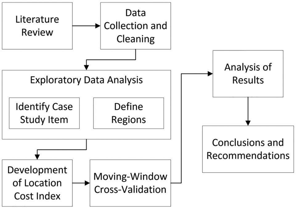
Research methodology.

Exploratory Data Analysis

The EDA is an approach used in data analysis to perform an initial review of one or multiple datasets. In this particular study, EDA was used to better understand each of the variables contained in the available data, as well as the relationships among them. It also allowed for the identification of the case study item. The selected HMA pay item was clearly identified as the most relevant in terms of frequency of use and dollar expenditure: “Superpave Bituminous Concrete Wearing Surface Layer, 1/2” Maximum Aggregate Size Mix – Item ID 424A360.” This pay item corresponds to the second highest dollar expenditure in ALDOT’s annual construction program. It is only outranked by mobilizations expenses, which are paid by ALDOT in almost all construction contracts, including non-paving projects, which could explain why this is the top-ranked item.

The better understanding of the data gained through the EDA was also used to split the historical bid data into comparable regions for the development of the HMA-LCI. Each region was required to provide sufficient data to allow for a reliable analysis, and at the same time, they could not be so large that they would become meaningless geographic-wise. The study initially considered the five geographic regions used by ALDOT to organize its operations: north (N), east-central (EC), west-central (WC), south-central (SC), and south-west region (SW). Figure 2 shows the partition of the state of Alabama according to these five regions.

Figure 2.

ALDOT geographic regions: Five-region classification.

The decision to use this partition had to be reevaluated when the EDA revealed that some of these regions were not providing a constant stream of HMA pricing data along the period of time considered in this study. More specifically, the regions providing the lowest count of paving projects per quarter are the WC and SW regions. This issue was solved by rearranging this partition into three regions: north, central, and south region. The final partition is shown in Figure 3.

Figure 3.

Final geographic regions: three-region classification.

Development of Location Cost Index

To develop the HMA-LCI, the authors first identified an actual typical paving project awarded by ALDOT, took the quantity of HMA estimated for that project (8,715 tons), and used the collected bid data to determine the annual average unit price that would actually be paid by ALDOT for that amount of HMA in each region between 2006 and 2016. Figure 4 shows how the unit price for 8,715 tons of HMA changed across these 11 years in each region.

Figure 4.

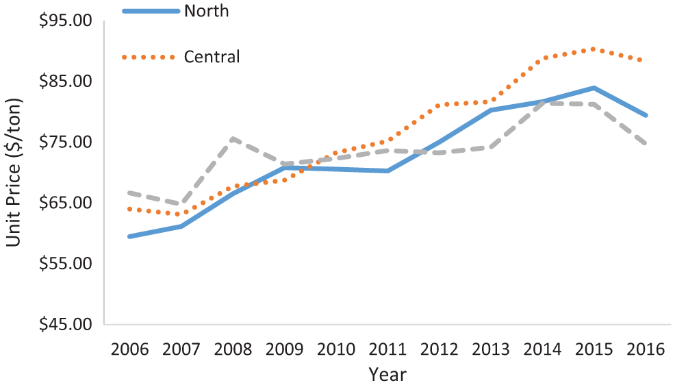
Hot mix asphalt unit price per region 2006–2016.

Average unit prices illustrated in Figure 4 were estimated by developing non-linear regression models such as the one shown in Figure 5, correlating quantities of work and unit prices for the HMA item under consideration on an annual basis for every year between 2006 and 2016. These non-linear regression equations represent the average quantity–unit price relationship for this item during each year. Thus, a unit price estimated with one of these equations for 8,715 tons of HMA can be reasonably assumed to represent the average unit price for that quantity of work during its corresponding year.

Figure 5.

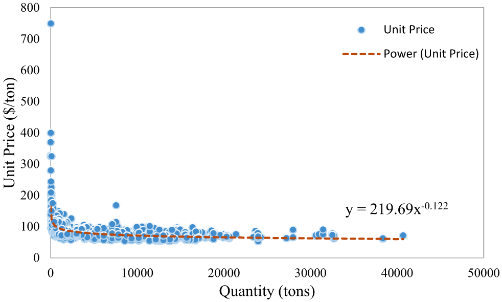
Quantity–unit price relationship for HMA (Pay item 424A360).

The next step was to determine if there are significant differences between the three-time series in Figure 4. A LCI would not be necessary if no significant differences are found. A visual inspection of this figure seems to show that HMA prices across the three regions started to increasingly spread out after 2010. A series of ANOVA tests applied to different time frames were used to validate this statement. The results of these tests are presented in Table 1.

Table 1.

ANOVA Test Results to Compare Average Unit Prices per Region

Years	Time frame	Region	Average unit price	p-value	Conclusion
11	2006–2016	North	67.05	0.607	No enough information to prove a significant difference with a significance level of 5%
		Central	74.74
		South	73.00
10	2007–2016	North	68.41	0.549
		Central	76.15
		South	74.12
9	2008–2016	North	69.90	0.394
		Central	77.87
		South	75.31
8	2009–2016	North	71.36	0.215
		Central	79.19
		South	74.96
7	2010–2016	North	72.43	0.076
		Central	81.27
		South	75.66
6	2011–2016	North	73.72	0.034	Significant difference with a significance level of 5%
		Central	82.86
		South	76.44
5	2012–2016	North	75.48	0.005
		Central	84.41
		South	77.37
4	2013–2016	North	76.59	0.007
		Central	84.89
		South	78.57
3	2014–2016	North	76.42	0.018
		Central	86.29
		South	79.58

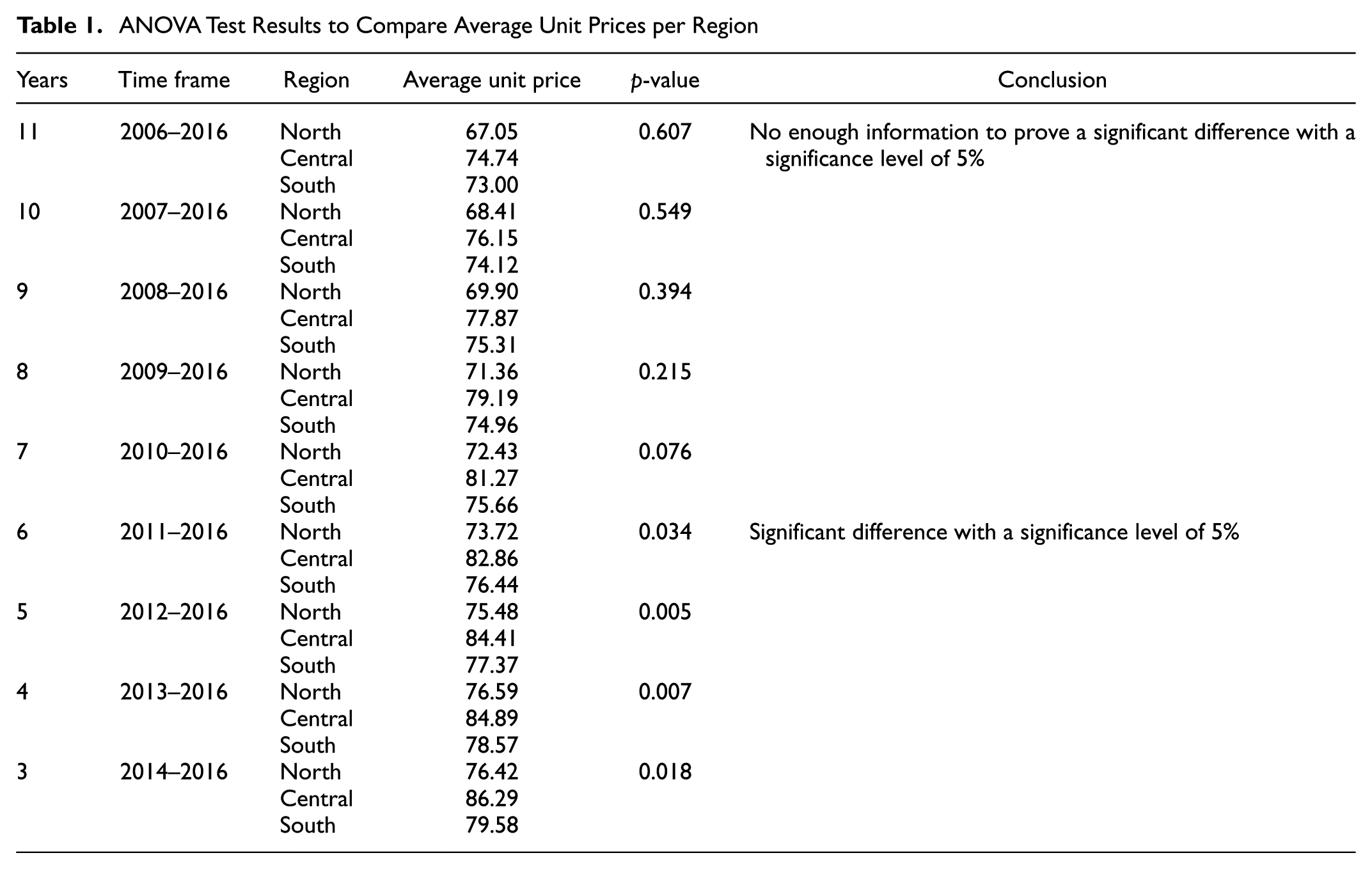
The first test was conducted to compare the 11-year average unit price (2006–2016) between the three regions, and it revealed no significant difference with a significance level of 5% (p-value = 0.05). The timeframe was then reduced by 1 year (2007–2016) and the ANOVA test was run again with the same results. The process was repeated several times, reducing the time frame by 1 year at a time, showing that significant differences between the regions started to appear after 2010.

Two important findings were derived from the statistical analysis described above. First, it can be assumed that current HMA prices may change significantly between regions. The second finding is that some sort of event(s) may have happened in 2010 affecting the paving construction market in Alabama. Therefore, the authors decided to continue developing the proposed system and to validate it using only data from projects awarded between 2011 and 2016 because old HMA pricing trends may affect the results of this study, misleading ALDOT on the expected performance of the proposed system in today’s construction industry. Thus, the authors proceeded to develop a LCI to quantity the difference between these regions at each year, starting in 2011.

The LCI was developed following a similar approach as the one adopted by the RSMeans for the calculation of its City Cost Index ( 23 ). The RSMeans City Cost Index compares average construction costs among 731 U.S. and Canadian Cities. The index values for all U.S. cities are calculated using the U.S. national average as a reference. Every year, the U.S. national average is assigned an index value of 100, and index values for each city are calculated in a proportional manner using the national index as a reference. Thus, if, for example, the index value for a given city is 95, that would mean that average construction costs in that city are 5% lower than the national average. Likewise, an index value of 102 would mean that average costs for that city are expected to be 2% above the national average.

Figure 6 shows the same time series from Figure 4, by adding one more time series for the state average HMA unit price for 8,715 tons of HMA. The values plotted in this figure for each region were compared against the state average of their respective years. The results of these comparisons were then translated into index values in a similar fashion as in the RSMeans City Cost Index. The resulting LCI is shown in Table 2.

Figure 6.

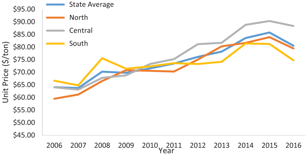
Hot mix asphalt unit price per region and state average 2006–2016.

Table 2.

HMA Location Cost Index for Alabama

Year	State	North	Central	South
2011	100.00	95.15	102.56	100.21
2012	100.00	97.53	106.98	96.35
2013	100.00	102.02	104.51	94.93
2014	100.00	97.12	106.75	97.37
2015	100.00	97.80	105.70	94.22
2016	100.00	98.46	110.25	92.42

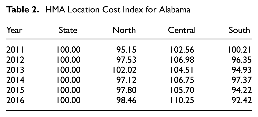
Although there does not seem to be a clear pattern to define the difference in HMA prices between the north and south regions, Figure 6 and the LCI in Table 2 show a clear trend of higher HMA prices in the central region in comparison with the other two regions. On average among the 6 years shown in Table 2, HMA prices in the central region are 8.3% and 10.8% higher than those in the north and south regions, respectively. Further research is required to attempt to explain the reason behind the price difference between regions. However, these results were discussed during a face-to-face meeting with ALDOT’s staff involved in cost-estimating tasks, and they expressed no surprise about these results, explaining that ALDOT has been perceiving that HMA prices have been growing at a greater rate in those counties located in the central region.

Moving-Window Cross-Validation

After developing the HMA-LCI, the next step was to assess the performance of this index as a cost-estimating input in the estimation of unit prices for the case study item, and it was done through the application of the MWCV algorithm. This algorithm has previously been used by the authors to assess the performance of a bid-based cost-estimating methodology designed to account for project scale and time effects on the estimation of unit prices for the same case study item ( 4 ). Project scale and time effects were factored into the cost-estimating process using non-linear regression and cost-indexing techniques. The MWCV algorithm was also used in that study to determine the optimal amount of historical data required to maximize estimating effectiveness for the case study item. It was found that highest estimating performance for the case study item was obtained using 2 years of previous bid data. A “before” versus “after” comparison, similar to the one described earlier in this paper, revealed a statistically significant improvement in cost-estimating effectiveness after incorporating the cost index to counteract time affects in bid-based estimating. The validation process for the HMA-LCI proposed in this paper is performed on the results from the previous study described in this paragraph in order to determine if cost-estimating effectiveness would improve even more after adjusting the previously calculated unit prices with the LCI and according to their respective project locations. It must be noted that unit price estimations in the previous study were calculated with bid data from projects executed all across the state; therefore, these are state average estimates. Detailed information about the research methodology and results from these previous research efforts can be found in Pakalapati ( 4 ).

The MWCV algorithm used in this study is an advanced version of cross-validation techniques commonly used to assess the performance data-driven construction cost-estimating systems. A typical cross-validation process is performed in four general steps: (1) the available data are split into a training and a testing dataset; (2) the training dataset is then used to develop the model; (3) the model is applied to the testing dataset to estimate the values of the independent variable(s) on each observation; and finally, (4) the estimated values are compared against the actual values of the independent variable(s) in the testing dataset, and the result of this comparison is analyzed to assess the performance of the model. The cross-validation process is intended to simulate the actual implementation of the model, so that the cross-validation results are assumed to reflect the level of performance that should be expected by the final users. However, the literature review has revealed some major issues with traditional cross-validation approaches that may compromise the integrity of the validation results. A complete description of the MWCV approach used in this study and the limitations of traditional cross-validation techniques is presented by Pakalapati ( 4 ).

The MWCV algorithm is illustrated in Figure 7. In this study, the moving-window refers to the two-year window (optimal amount of data previously determined by the authors) moving across the testing projects (projects used to assess the performance of the proposed methodology), which in this case consist of all 97 project using the case study item during 2016. The MWCV process places the end of the two-year window at the beginning of the testing period (January 2016), and then starts moving toward the end of the testing timeline. Every time that the right-end of the moving-window finds a project, it stops, the HMA unit price for that project is estimated, and the APE is calculated; then the moving-window continues its way until finding the next project. At the end of the MWCV process, the MAPE and standard deviation of all APEs are calculated to determine the overall accuracy and reliability of the system. The MWCV algorithm allows us to calculate the MAPE and standard deviation values that ALDOT would have experienced if the proposed cost-estimating methodology were actually used to estimate unit prices for a set of projects in the past, which is not possible with traditional cross-validation techniques.

Figure 7.

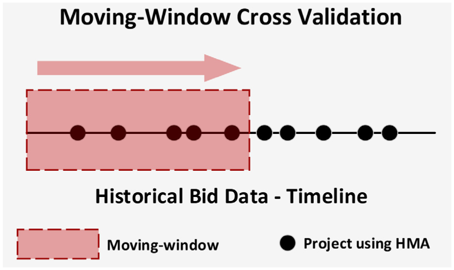
Moving-window cross-validation algorithm.

Analysis of Results

Table 3 shows the APEs for all 97 testing projects before and after using the LCI. The “before” APEs were using the state average unit price estimates from the previous study and Equation 1. On the other hand, the “after” APEs were also calculated with Equation 1, but after adjusting all unit prices with the LCI. Location adjustments of state average estimates were performed as shown in Equation 3 and using the index values from Table 2 for 2016.

LAUP = SAUP \times \frac{LICR}{100}

(3)

where: LAUP = Location-Adjusted Unit Price

SAUP = State Average Unit Price

LICR = Location Index in Current Region

Table 3.

Moving-Window Cross-Validation: Summary of Results

Project	Region	APE “Before”	APE“After”	Project	Region	APE“Before”	APE“After”	Project	Region	APE“Before”	APE“After”
1	C	41.0%	37.6%	34	S	25.0%	17.8%	67	N	3.6%	5.7%
2	N	0.2%	2.4%	35	C	9.9%	16.2%	68	S	19.0%	12.1%
3	S	13.6%	7.0%	36	C	21.6%	28.5%	69	N	12.8%	10.3%
4	N	2.0%	0.2%	37	C	10.0%	4.8%	70	S	3.8%	2.2%
5	S	6.7%	0.6%	38	C	17.5%	12.8%	71	S	7.7%	1.5%
6	S	5.6%	11.0%	39	N	14.0%	11.5%	72	N	17.9%	15.3%
7	C	18.7%	14.1%	40	N	4.3%	6.4%	73	C	21.9%	28.9%
8	N	21.6%	23.4%	41	S	4.5%	1.6%	74	S	21.0%	14.0%
9	N	8.1%	5.7%	42	C	2.1%	3.4%	75	C	24.2%	19.8%
10	S	3.4%	9.0%	43	S	13.5%	6.9%	76	C	8.0%	14.1%
11	S	18.4%	11.6%	44	C	12.5%	18.9%	77	S	1.9%	7.6%
12	C	16.9%	23.6%	45	C	16.3%	22.9%	78	N	21.8%	23.5%
13	S	7.8%	13.2%	46	N	28.3%	29.8%	79	S	7.3%	1.1%
14	N	4.0%	6.1%	47	C	15.9%	11.1%	80	S	12.7%	6.2%
15	S	12.1%	17.2%	48	N	20.4%	17.7%	81	C	7.8%	2.5%
16	S	5.9%	0.2%	49	S	9.2%	2.9%	82	N	12.8%	10.3%
17	N	16.1%	13.6%	50	N	4.5%	2.2%	83	C	5.9%	0.5%
18	C	9.6%	4.5%	51	N	8.0%	10.0%	84	N	25.1%	22.4%
19	S	7.1%	12.5%	52	C	2.1%	3.4%	85	C	13.7%	8.7%
20	C	21.6%	28.5%	53	S	31.4%	35.4%	86	C	2.6%	2.9%
21	S	11.4%	16.5%	54	S	9.6%	3.2%	87	S	21.3%	25.8%
22	S	6.5%	0.3%	55	C	14.2%	20.7%	88	S	2.0%	3.9%
23	N	8.5%	6.1%	56	C	5.5%	0.1%	89	N	13.9%	11.4%
24	N	10.6%	8.2%	57	S	27.8%	31.9%	90	N	19.0%	16.4%
25	N	33.2%	30.3%	58	C	7.3%	2.0%	91	C	8.2%	14.3%
26	S	24.1%	16.9%	59	C	13.0%	8.0%	92	S	7.0%	0.9%
27	S	18.7%	23.4%	60	C	12.2%	7.2%	93	C	18.8%	14.2%
28	S	9.7%	15.0%	61	C	20.9%	16.3%	94	S	6.5%	0.4%
29	C	4.6%	0.8%	62	S	12.6%	6.1%	95	S	2.0%	7.7%
30	C	10.4%	5.3%	63	S	9.4%	3.0%	96	S	1.3%	4.6%
31	C	18.6%	13.9%	64	N	4.1%	1.8%	97	C	25.5%	21.3%
32	S	18.1%	11.3%	65	C	3.8%	1.6%	MAPE		12.5%	11.3%
33	S	9.3%	3.0%	66	C	1.6%	7.4%	SD of APEs		8.2%	9.1%

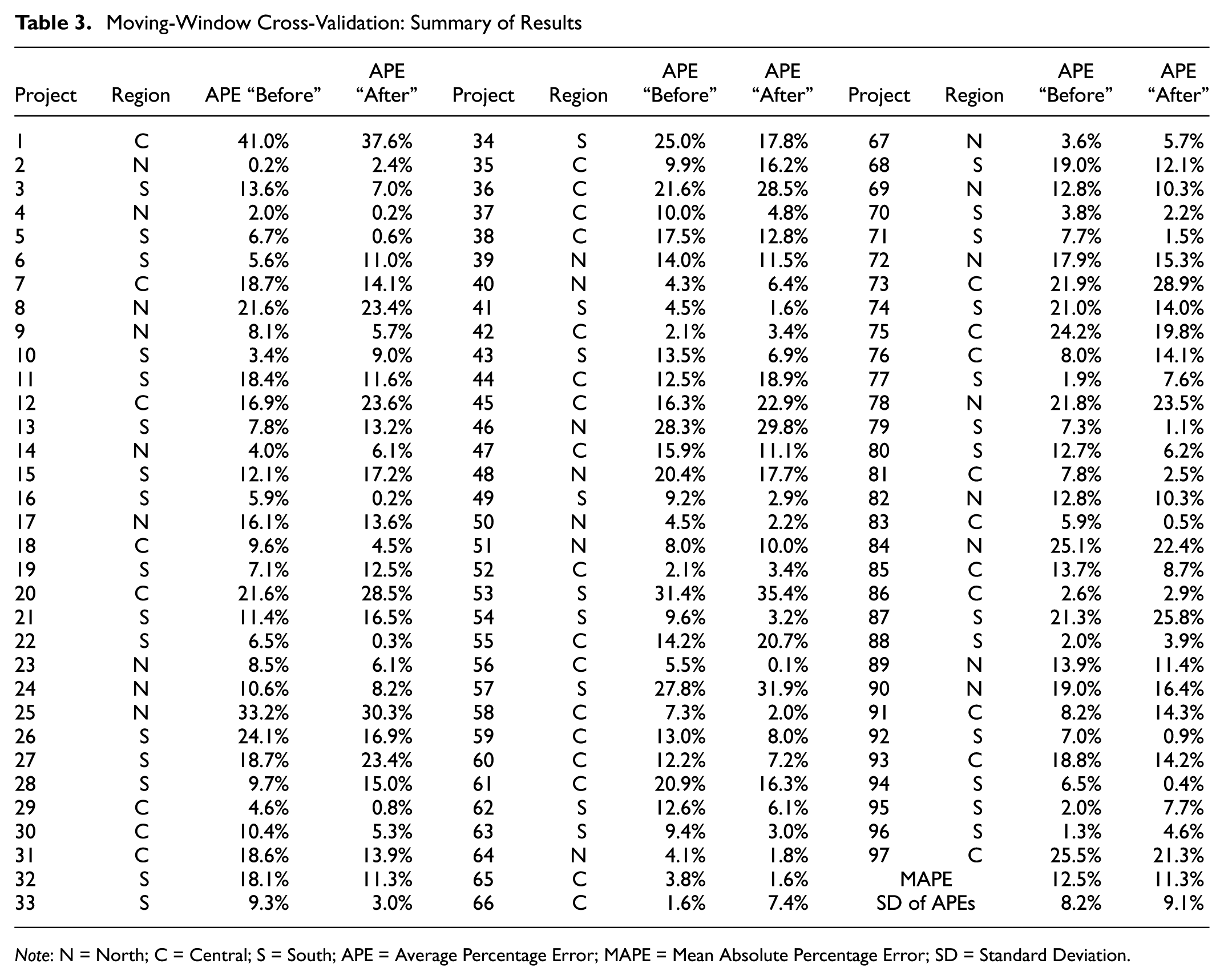
Note: N = North; C = Central; S = South; APE = Average Percentage Error; MAPE = Mean Absolute Percentage Error; SD = Standard Deviation.

Table 3 shows that the use of the proposed LCI to counteract location effects was able to improve cost-estimating accuracy even more, by reducing the MAPE by 9.6% ([0.125–0.113]/0.125 × 100%). A statistical paired two-sample t-test demonstrated that this was a significant improvement in accuracy with a 1% significant level. On the other hand, the results show an increase in the standard deviation of the APEs, which would suppose a reduction of 11.0% ([0.082–0.091]/0.082 × 100%) in the level of reliability after using the LCI. However, a statistical F-test did not show this reduction as statistically significant. Therefore, this study can conclude that the implementation of the LCI would have a significant positive impact on ALDOT’s construction cost-estimating accuracy without affecting estimating reliability.

Conclusions and Recommendations

This paper has presented the research efforts undertaken for the development of an annual HMA-LCI, intended to compare construction prices across three different regions in Alabama (north, central, and south) and to adjust cost estimates according to the geographic location of each project. Data collection, cleaning, and analysis procedures presented throughout this paper were conducted using historical bid data from all projects awarded by ALDOT between 2006 and 2016 (3,661 projects). The potential contribution of the proposed LCI to improving ALDOT’s current cost-estimating practices was demonstrated using a MWCV algorithm and statistical significance testing techniques. The impact of the proposed LCI on cost estimating was defined in terms of accuracy and reliability, measured by MAPEs and standard deviation values of APEs, respectively. The MWCV algorithm revealed a reduction in estimating reliability after including the LCI into the cost-estimating process. However, a statistical analysis showed that the increase in the standard deviation after adjusting unit price estimates for location impacts was not statistically significant, unlike the improvement in estimating accuracy observed between the same two sets of APEs (increase in MAPE value). This allows the authors to conclude that the location adjustments of unit price using the proposed LCI have a positive impact on cost-estimating effectiveness, by significantly improving accuracy without affecting estimating reliability.

Footnotes

Author Contributions

The authors confirm contribution to the paper as follows: Study conception and design: Keren Xu, Jorge Rueda-Benavides, and Karthik Pakalapati; Data collection: Keren Xu and Karthik Pakalapati; Analysis and interpretation of results: Keren Xu, Jorge Rueda-Benavides, and Karthik Pakalapati; Draft manuscript preparation: Keren Xu. All authors reviewed the results and approved the final version of the manuscript.

The Standing Committee on Construction Management (AFH10) peer-reviewed this paper (19-02672).

References

National Asphalt Pavement Association. Engineering Overview. 2018. http://www.asphaltpavement.org/

Rueda-Benavides

J. A.

Indefinite Delivery/Indefinite Quantity Project Selection Framework Using Stochastic Techniques. Doctoral dissertation. Iowa State University, 2016.

2018 Standard Specification for Highway Construction . Alabama Department of Transportation, 2018.

Pakalapati

K. C.

Data Usage Optimization for Cost Estimating in Asphalt Paving Projects Using a Cost Indexing System. Master’s thesis. Auburn University, 2018.

Report Card for Alabama’s Infrastructure - 2016 . American Society of Civil Engineers, 2015.

Alabama Asphalt Pavement Association. Asphalt Facts. 2016. http://alasphalt.com/asphalt-facts/

Project Management Institute (PMI). A Guide to the Project Management Body of Knowledge (PMBOK Guide), 5th ed. ANSI/PMI 99-001-2013. Project Management Institute, Inc., 2013.

Practical Guide to Cost Estimating. American Association of State Highway and Transportation Officials, 2013.

Fakultesi

Zeynep

A Neural Network Approach for Early Cost Estimation of Structural Systems of Buildings. International Journal of Project Management, Vol. 22, No. 7, 2004, pp. 595–602.

10.

Arafa

Alqedra

Early Stage Cost Estimation of Buildings Construction Projects using Artificial Neural Networks. Journal of Artificial Intelligence, Vol. 4, No. 1, 2011, pp. 63–75.

11.

Byrnes

J. E.

Best practices for highway project cost estimating. Arizona State University, Tempe, 2002.

12.

Golafshani

Understanding Reliability and Validity in Qualitative Research. The Qualitative Report, Vol. 8, No. 4, 2003, pp. 597–606.

13.

Gardner

B. J.

Gransberg

D. D.

Jeong

H. D.

Reducing Data-Collection Efforts for Conceptual Cost Estimating at a Highway Agency. Journal of Construction Engineering and Management, Vol. 142, No. 11, 2016, 04016057.

14.

American Society of Civil Engineers (ASCE). Pricing and Bidding: Unit Price Jobs. Construction Engineering Certificate Program, 2017.

15.

Betts

Standardization in Information Technology Industries: Emerging Issues under Section Two of the Sherman Antitrust Act. Oklahoma Journal of Law and Technology, Vol. 3, No. 1, 2007, 6p.

16.

Zhang

Sun

Economic Potential of Modular Reactor Nuclear Power Plants Based on the Chinese HTR-PM Project. Nuclear Engineering and Design, Vol. 237, No. 23, 2007, pp. 2265–2274.

17.

Akintoye

Analysis of Factors Influencing Project Cost Estimating Practice. Construction Management & Economics, Vol. 18, No. 1, 2000, pp. 77–89.

18.

Akanni

P. O.

Oke

A. E.

Akpomiemie

O. A.

Impact of Environmental Factors on Building Project Performance in Delta State, Nigeria. HBRC Journal, Vol. 11, No. 1, 2015, pp. 91–97.

19.

Cuervo

J. C.

Sui Pheng

Significance of Location Factors for Singapore Transnational Construction Corporations. Engineering, Construction and Architectural Management, Vol. 10, No. 5, 2003, pp. 342–353.

20.

Kaming

P. F.

Olomolaiye

P. O.

Holt

G. D.

Harris

F. C.

Factors Influencing Construction Time and Cost Overruns on High-Rise Projects in Indonesia. Construction Management & Economics, Vol. 15, No. 1, 1997, pp. 83–94.

21.

Skamris

M. K.

Flyvbjerg

Inaccuracy of Traffic Forecasts and Cost Estimates on Large Transport Projects. Transport Policy, Vol. 4, No. 3, 1997, pp. 141–146.

22.

Dikmen

Birgonul

M. T.

Gur

A. K.

A Case-Based Decision Support Tool for Bid Mark-up Estimation of International Construction Projects. Automation in Construction, Vol. 17, No. 1, 2007, pp. 30–44.

23.

RSMeans. Building Construction Costs with RSMeans Data: 76th Annual Edition. Gordian Group, LLC, 2018.