
Abstract
Freight demand models typically employ a priori classification systems for dividing establishments into hypothetically complementary groups with homogeneous patterns in freight production (FP) and freight trip production (FTP). Although an attractive and popular notion, the assumption of homogeneity within these a priori industrial classes is reductive in nature and is not yet tested in literature. This research examines this hypothesis and explores the possibility of a data-driven segmentation by examining the relationships between FP/FTP patterns and prevalent a priori classes; subsequently, it creates homogeneous ensembles of a posteriori segments through aggregation. This research labels, explains, and interprets these novel segments using commodity value density of industrial classes. The alternate segmentation schemes are compared in their ability to predict FP and FTP and it is found that: (i) industrial classification systems (NAICS, ISIC) perform significantly better than product classification systems (ASICC); (ii) a considerable portion of variability in FTP does not depend on employment predictor due to the underlying influence of shipment size; (iii) an a posteriori segmentation scheme considering shipment size may represent an effective middle ground for developing both FP and FTP models in freight demand model systems. Adoption of these novel segments of the freight travel market has the potential to reduce the sample size requirements of freight demand model systems and minimize the financial necessities for future freight surveys.
The highly competitive business environment in the era of market-driven globalization has motivated considerable research towards developing freight transportation planning tools at both national and local scales ( 1 ). The growth of this research is reflected even in developing economies where freight movements are no longer dismissed as an afterthought of the planning process due to the strong incentives for reducing the generalized cost of moving goods and improving the speed of delivery of goods to consumers ( 2 ). Transportation planners and practitioners are entrusted with the responsibility of developing effective freight mobility enhancement initiatives founded on quantitative freight demand models. These freight demand models are expected to provide answers to relevant planning concerns, such as: What are the traffic impacts or freight needs of commercial developments? What are the differential effects of freight-specific policy instruments (access time regulations, night-time delivery systems) on various industry sectors? And how to design and evaluate the feasibility of large-scale investments for planning dedicated freight corridors, truck-exclusive lanes, etc.? In short, freight demand models are crucial for agencies and government authorities that seek decision-making tools directed towards regulating or enhancing the current state of urban freight movements. Notwithstanding these substantial applications, research focused on quantifying urban freight movements has been modest at best ( 3 ).
The popular models provided in existing freight demand model systems to anticipate traffic impacts and predict future patterns are freight trip generation (FTG) and freight generation (FG) models ( 4 ). In both FG and FTG, classification of establishments is a crucial step for improving the model quality and organizing the models in such a way that they complement the forecast requirements of land-use ordinances and policy interventions ( 5 ). Classification systems improve the model quality because establishments within a group share common characteristics, which reduces the internal variability of data in that group. Given the economic nature of models, classification is even more necessitated by the fact that the ability of business size predictors, such as employment, to predict FG/FTG would be challenged if there were internal disparity in the economic activity performed by the establishments. Even in cases where data segmentation is not feasible due to limited sample sizes, FG/FTG models are estimated using binary variables denoting industrial sectors ( 3 ). There has thus been a growing interest lately in identifying the most suitable classification system which leads to homogeneous classes of establishments with similar freight travel patterns ( 1 , 4 , 6 ). An examination of the literature revealed that the previous studies have predominantly used an a priori classification approach, rather than the data-driven a posteriori segmentation approach. While a priori classification refers to the process of grouping establishments into pre-defined labels (e.g. NAICS in the U.S.A.), a posteriori segmentation refers to the data-driven process of identifying conceptually meaningful subgroups of homogeneous freight travel (FG/FTG) patterns. An a priori classification is, in effect, a decision or a forced choice which assumes that there is some knowledge in advance about the homogeneous classes of FG/FTG patterns and they are distinguishable by existing descriptors of land-use, economic (industrial) activity, etc. Although an attractive and popular notion, the validity of this rather reductive assumption is rarely tested in the freight literature. The different a priori classification systems exhibit varying degrees of ability to capture the minimum intra-variability groups in terms of FG/FTG. Land-use classification systems, for instance, are reported to be inferior to industrial (economic) classification systems in their ability to estimate FG/FTG models since land-use classes are often aggregate in nature and consist of an agglomeration of disparate economic sectors ( 5 ).
The selection of a priori industrial classification systems for freight data segmentation is an intricate issue due to the presence of a large variety of non-integrated classification codes existing in each country or continent. Among the alternatives in the U.S.A. there is a general consensus that NAICS codes lead to better freight trip production (FTP) models whereas SIC codes produce better freight trip attraction (FTA) models ( 1 ). The generalizability of this finding to other countries is questionable, however, since there is cross-continental and, more often, cross-national variation in the codal structure of classification systems. The lack of concordance in classification systems is conveyed in a recent study by Gonzalez-Feliu et al. ( 7 ) which reported that diverse FTG patterns coexist within eight selected classes of the French NAF industrial classification system. This finding underlines the crucial necessity of developing a data-driven a posteriori segmentation using establishment-level data grouped into a priori classes. In order to address these research gaps in the area of freight data segmentation, this paper uses data from a comprehensive establishment-based freight survey (EBFS) targeted at shippers in India and focuses on freight production (FP) and FTP. The main objective of this paper is to explore the relationships between FP/FTP patterns and prevalent a priori industrial classification systems. Based on the similarities and dissimilarities, a priori industrial classes are aggregated to form homogeneous ensembles of a posteriori segments. The identification of these novel segments of freight travel market has the potential to: (i) reduce the sample size implications of developing numerous separate FP/FTP models; (ii) reduce the time and cost for future freight surveys by acting as the base for alternative sampling methods. The paper also compares both a priori classification systems and a posteriori segmentation schemes in terms of their ability to predict FP and FTP.
This paper is structured in four sections following this introduction. The next section gives an overview of the best practices on industrial classification systems used in the context of freight demand models. The research design, data, and methodological approach are presented in the third section. The model estimation results are discussed in detail in the fourth section, and paper ends with conclusions.
Industrial Classification Systems
The assumption that homogeneous FG/FTG patterns exist among establishments grouped using various industrial classification systems, an attractive and popular notion, stretches back to early freight studies. Though reductive in nature, this assumption is based on the intuitive reasoning that the long-term decisions of an establishment are determined by its economic activity, commodity type, and land-use type ( 8 ). Instead of estimating generic freight demand models for establishments, researchers have used the available a priori industrial classification systems to group establishments and organize the models ( 5 ). The various industrial classification systems around the world are presented in Table 1 with due focus given to explanations of their codal structure. The classification systems are explained in detail below. The interdependence among industrial and product classification systems is illustrated in Figure 1.
Details of Industrial Classification Systems Adopted for A Priori Classification of Establishments
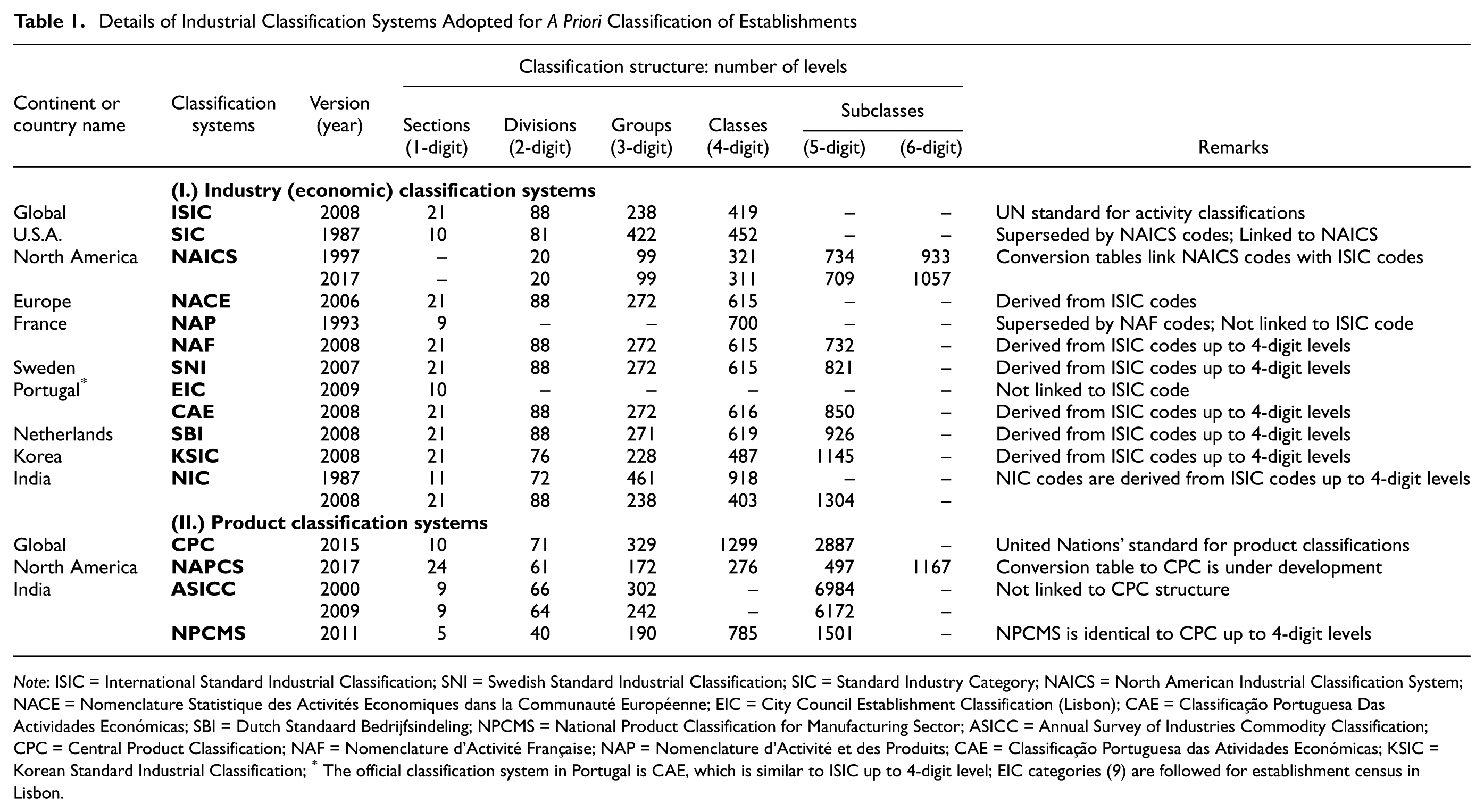
Note: ISIC = International Standard Industrial Classification; SNI = Swedish Standard Industrial Classification; SIC = Standard Industry Category; NAICS = North American Industrial Classification System; NACE = Nomenclature Statistique des Activités Economiques dans la Communauté Européenne; EIC = City Council Establishment Classification (Lisbon); CAE = Classificação Portuguesa Das Actividades Económicas; SBI = Dutch Standaard Bedrijfsindeling; NPCMS = National Product Classification for Manufacturing Sector; ASICC = Annual Survey of Industries Commodity Classification; CPC = Central Product Classification; NAF = Nomenclature d’Activité Française; NAP = Nomenclature d’Activité et des Produits; CAE = Classificação Portuguesa das Atividades Económicas; KSIC = Korean Standard Industrial Classification; * The official classification system in Portugal is CAE, which is similar to ISIC up to 4-digit level; EIC categories ( 9 ) are followed for establishment census in Lisbon.
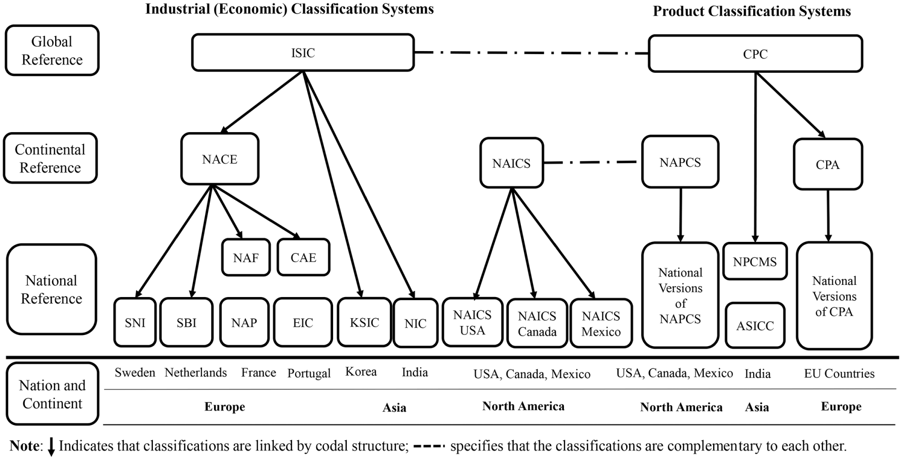
Linkages between existing classification systems.
International Standard Industrial Classification System (ISIC)
ISIC is a global standard for classification which groups establishments according to their economic activity ( 10 ). ISIC classifies industries using a four-digit hierarchical structure, in which the categories at the highest level are called sections (denoted by letters A to U), followed by divisions (two-digit level), groups (three-digit level) and classes (four-digit level). The majority of countries around the world have used ISIC as the base for developing national classifications to enable comparisons of economic data. The ISIC system categorizes establishments into 13 industry sectors as follows: (1) ISIC:10: Food products, (2) ISIC:11: Beverages; (3) ISIC:13: Textile mills, (4) ISIC:14: Wearing apparel, (5) ISIC:16: Wood, wood products, furniture, and fixtures, (6) ISIC:17–18: Paper, paper products, and printing, (7) ISIC:20–21: Basic chemicals, chemical products, and pharmaceuticals, (8) ISIC:22: Plastic and rubber products, (9) ISIC:23: Non-metallic mineral products, (10) ISIC:24–25: Basic metal, alloy, metal products, (11) ISIC:26–28: Machinery and equipment, (12) ISIC:29–30: Transportation equipment, and (13) ISIC:32: Other manufacturing industries.
The codal structure of Europe’s Nomenclature of Economic Activities (NACE), Korea’s Standard Industrial Classification (KSIC), and India’s National Industrial Classification (NIC) are completely in line with ISIC up to four-digit level ( 11 ). However, there is a wide variety of classification codes which are discordant with ISIC with some having limited comparability (NAP in France, EIC in Portugal), while others have conversion tables to produce comparable divisions to ISIC (NAICS in U.S.A., NAP in France).
North American Industrial Classification System (NAICS)
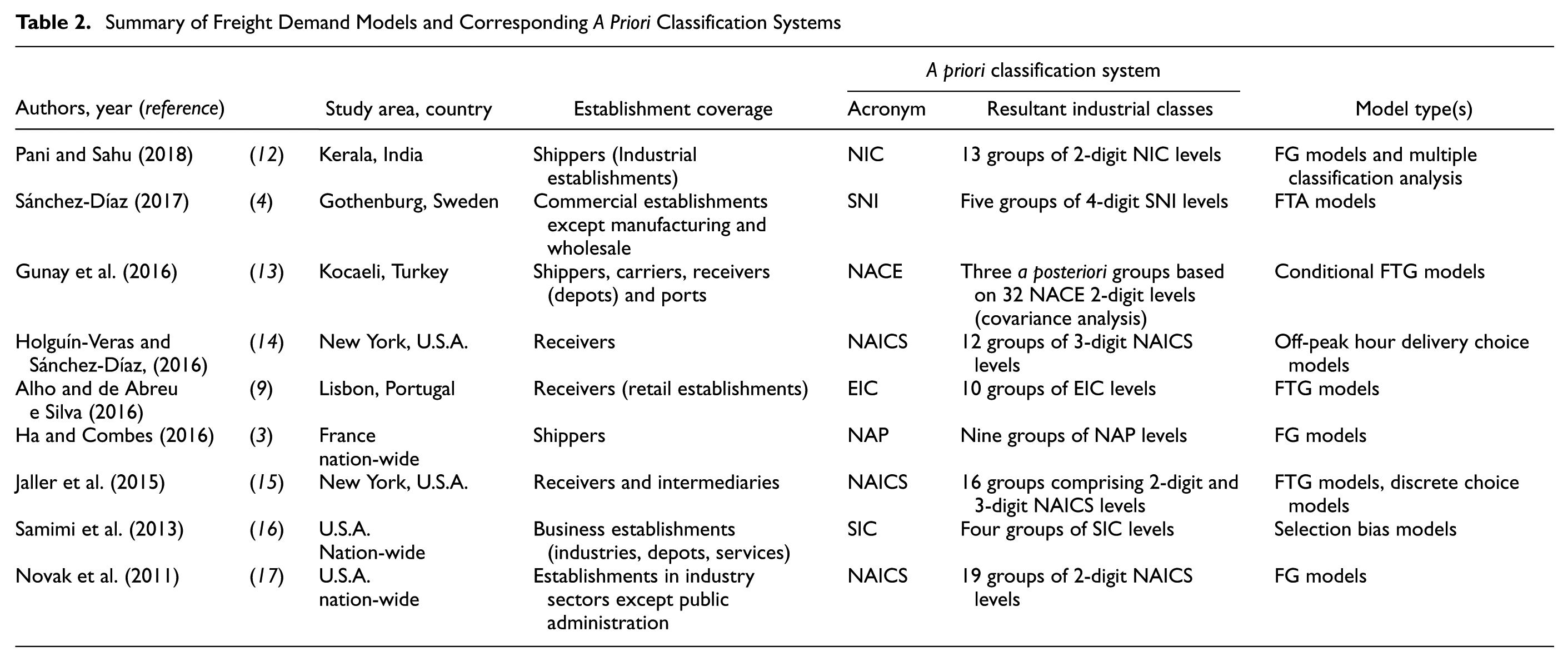
NAICS codes provide a consistent framework for industrial classification in North America ( 10 ). The classification system was erected on a production-oriented conceptual framework independent of the codal structure provided by ISIC. The NAICS codes are as follows: (1) NAICS:311 Food; (2) NAICS:312 Beverages and tobacco; (3) NAICS:313 Textile mills; (4) NAICS:314 Textile products; (5) NAICS:316 Leather and allied product manufacturing; (6) NAICS:321 Wood products; (7) NAICS:322 Paper products; (8) NAICS:323 Printing and related; (9) NAICS:325 Chemical; (10) NAICS:326 Plastics and rubber; (11) NAICS:327 Nonmetallic; (12) NAICS:331 Primary metal; (13) NAICS:332 Fabricated metal; (14) NAICS:333 Machinery; (15) NAICS 334 Computer and electronic products; (16) NAICS:335 Electrical equipment; (17) NAICS:336 Transportation equipment; (18) NAICS:337 Furniture products; (19) NAICS:339 Miscellaneous. A summary of freight demand models which have used various classification systems around the world is presented in Table 2. It can be seen that the origin of most of the classification system adopted in previous freight studies derives from either ISIC or NAICS. For instance, Pani and Sahu ( 12 ) estimated FG models and MCA tables for 13 two-digit NIC groups in India which, in turn, correspond one-to-one to the 13 two-digit ISIC groups.
Summary of Freight Demand Models and Corresponding A Priori Classification Systems
Annual Survey of Industries Classification System (ASICC)
Central Product Classification (CPC) is the product classification system sponsored by the United Nations to provide a global standard for categorizing products with alpha-numerical designations ( 18 ). CPC follows an industry-of-origin approach and therefore ISIC linkage exists for all CPC subclasses. Annual Survey of Industries Commodity Classification (ASICC) is a unique product classification system used in India for developing industrial databases (e.g., annual survey database maintained by district industries center). While the latest surveys follow NIC and CPC-based NPCMS, many of the available sources of industrial statistics in India are based on ASICC. Therefore, statistical investigation of the explanatory power of FP/FTP models using ASICC are of significant interest to freight research in a developing country like India. The ASICC codes are as follows: (1) ASICC:01 Animal, vegetable products, beverages, tobacco; (2) ASICC:02 Ores, minerals, gas, and electricity; (3) ASICC:03 Chemical and allied products; (4) ASICC:04 Rubber, plastic, and leather products; (5) ASICC:05 Wood, cork, paper products; (6) ASICC:06 Textile and textile articles; (7) ASICC:07 Base metals, machinery, equipment; (8) ASICC:08 Transport equipment (9) ASICC:09 Other manufactured products.
Research Design and Data
This section describes the research design adopted in this study. The first part describes the research data, and the second part elaborates the methodological approach and methods of analysis used in this study.
Data Description
The research is undertaken in Kerala, a strategically important state in India due to the presence of Cochin seaport which is one of the major gateways to international shipping traffic. The data used for analysis were collected through EBFS targeting shippers (manufacturing units, wholesalers, and raw material production sites) in seven cities in Kerala: Cochin, Calicut, Malappuram, Kannur, Palakkad, Thrissur, and Kottayam. The sampling frame for EBFS was developed using an economic census which provided a list of all industrial establishments in Kerala. The final sampling frame consisted of 54,170 establishments. Simple random sampling was adopted for EBFS since auxiliary information (e.g., industry sector, employment level) was missing for many records in the sample frame. The survey was administered by face-to-face interviews with logistics managers or firm owners of the establishments. The final sample comprises 432 establishments with complete observations. The response rate for the survey was 30.3%, which is marginally higher than the average response rate (28%) for past EBFS ( 19 ). Detailed information on the data collection plan, sampling design, response rates, and sample representativeness can be found in Pani et al. ( 2 ) and Pani and Sahu ( 12 ). The EBFS sample was originally coded using the ISIC system and it was recoded into other classification systems (NAICS and ASICC) for performing the analyses presented in this paper. The codal conversion was carried out at five-digit levels of NAICS and ASICC in order to avoid one-to-two correspondence between classification systems.
Methodological Approach and Analysis Methods
The research approach consists of three major parts. In the first part, a priori industrial classes (ISIC, ASICC, NAICS) are clustered into a posteriori segments using pair-wise comparisons of least significant difference as the test parameter. Three important aspects of freight movements are used for establishing these new segments: (i) FTP in trips/week; (ii) FP in tons/week, and (iii) shipment size (SS) in tons/shipment. Given a statistically significant difference in pair-wise comparisons (least significant difference test), industrial classes are not placed in the same a posteriori segment. If there is no statistically significant difference, they are appended in the same segment. This segmentation methodology is not intended to produce the best segmentation in terms of predictive accuracy or robustness, as compared with clustering algorithms (unsupervised learning methods). Instead, it is expected to offer practice-oriented segmentation schemes which sustain the applicability of FP/FTP models to external data still stored in a priori classes (e.g., employment statistics in NAICS). In the second part of the paper, the marginal means of industrial classes are used for graphical representation of a posteriori segments. The underlying patterns in these a posteriori segments are interpreted using an important physical characteristic of commodities handled by industrial classes: value density (value per 1 kg). The mean FTP/FP/SS of each a posteriori segment is compared with its mean value density. In the last part, the explanatory power of a priori and a posteriori segmentation schemes is compared using hierarchical linear models. The analysis methods are explained below.
Step 1: Least Significant Difference Test
Fisher’s least significant difference (LSD) test is a commonly used post-hoc test which comprises several independent pair-wise t-tests ( 20 ). The test uses a two-step procedure in which the first step is to conduct ANOVA tests and assess whether the groups are truly different from each other. Given a significant result in ANOVA tests, the second step is to calculate the smallest significant difference between all possible pairs of groups in the sample using Equation 1 as if a t-test had been run between that pair of means. The value of LSD is directly compared with the difference between two group means and the similarities or dissimilarities between the groups is assessed. That is, any difference larger than LSD is considered to be a significant result which rejects the null hypothesis that the groups are similar.

where
Step 2: Hierarchical Linear Modeling
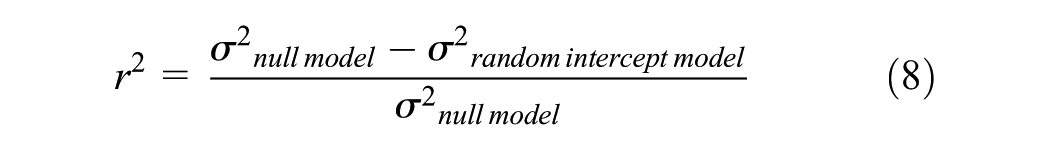
Hierarchical linear modeling (HLM) is a complex form of ordinary least squares regression that is used to predict the outcome variables that are grouped in hierarchical levels ( 21 ). For instance, establishments in an industrial class share variance among themselves (Level 1) and among the industrial classes (Level 2). HLM accounts for this shared variance in hierarchically structured data by estimating lower level (establishment) slopes and their variation in higher level outcomes (industrial classes). The model structure of this two-level HLM is explained in Equations 2–4. For the purpose of this analysis, two types of HLMs are estimated: unconstrained (null) models and random intercept models. The null model shown in Equation 5 estimates the variability in the outcome variable by level-2 groups and suggests whether HLM is valid or not. The results for the null model include the intra-class correlation coefficient (ICC) which determines the percentage of variance in outcome variable that is attributable to group membership (i.e., industrial classes). The expression for ICC is given in Equation 6. Subsequently, random intercept models given in Equation 7 are developed to analyze the relationship between level-1 predictor (i.e., employment) and the grouped outcome variable. In these models, the measure of variance explained by level-1 predictor variable (r2) is computed using Equation 8 and compared for different industrial classification systems.
HLM model structure

Intercept for jth level-2 unit

Coefficient for jth level-2 unit

Unconstrained (null model)


Random intercept model

where
Results and Discussion
A Posteriori Segmentation Based on FTP and FP
The starting point of this approach is to assign the population of establishments to subgroups using a priori classification systems such as ISIC, ASICC, and NAICS. The a priori classes are subsequently clustered using LSD test. The model estimation results and their interpretations are discussed in the sub-sections below.
ISIC-Based Segmentation
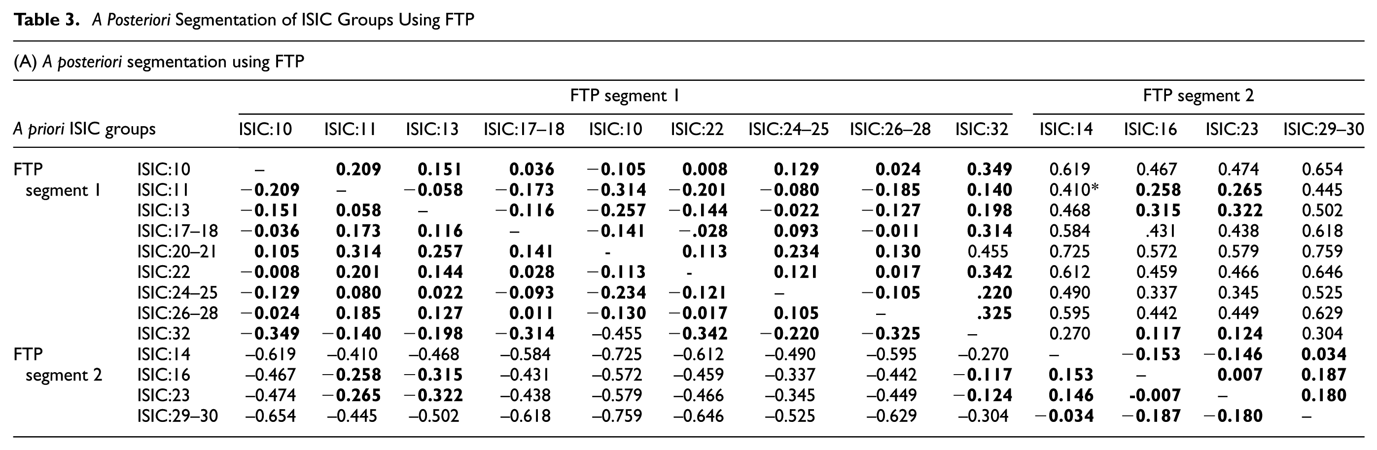
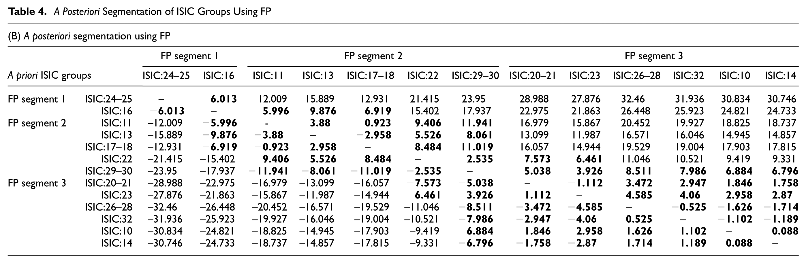
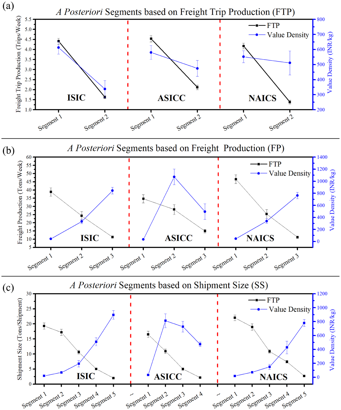
Levene’s test was first conducted to test the homogeneity of variances of outcome variables, here, FTP and FP. The test results for FTP showed that variances are not equally distributed since the significance values were very close to zero. This result may be due to the skewed distribution of FTP. This necessitated taking natural logarithms of FTP as a variance stabilizing transformation. Levene’s test was performed again for the logarithmically transformed variable (lnFTP) which led to a test statistic value of 0.463 (significance = 0.936). This indicates that the null hypothesis of equality of error variances for ln(FTP) cannot be rejected at significance value of 0.05 and that the application of ANOVA procedure is valid. On the other hand, test results for FP showed that variances are equally distributed (significance = 0.732) without any variable transformations. Subsequently, pair-wise comparisons of the ISIC groups were made by LSD test. The results of LSD test for both ln(FTP) and FP are presented in Tables 3 and 4. The ISIC groups which do not have insignificant differences are grouped together, as shown in boldface numbers. The ordering of groups is modified to distinguish the appended groups. In the case of FTP, the results of LSD test led to two segments, whereas FP led to three segments. It should be noted that a few ISIC groups such as ISIC:16 and ISIC:23 show FTP similarities to some groups in segment 1, despite being placed in segment 2; however, since these groups do not have FTP similarities with other groups in segment 1, they are placed in segment 2. Similar atypical similarities can be found in the case of FP segments as well. The segment divisions are graphically presented in Figure 2a and 2b using marginal means plots. The marginal means show the variation of mean FTP or FP for each ISIC group within each main segment.
A Posteriori Segmentation of ISIC Groups Using FTP
A Posteriori Segmentation of ISIC Groups Using FP
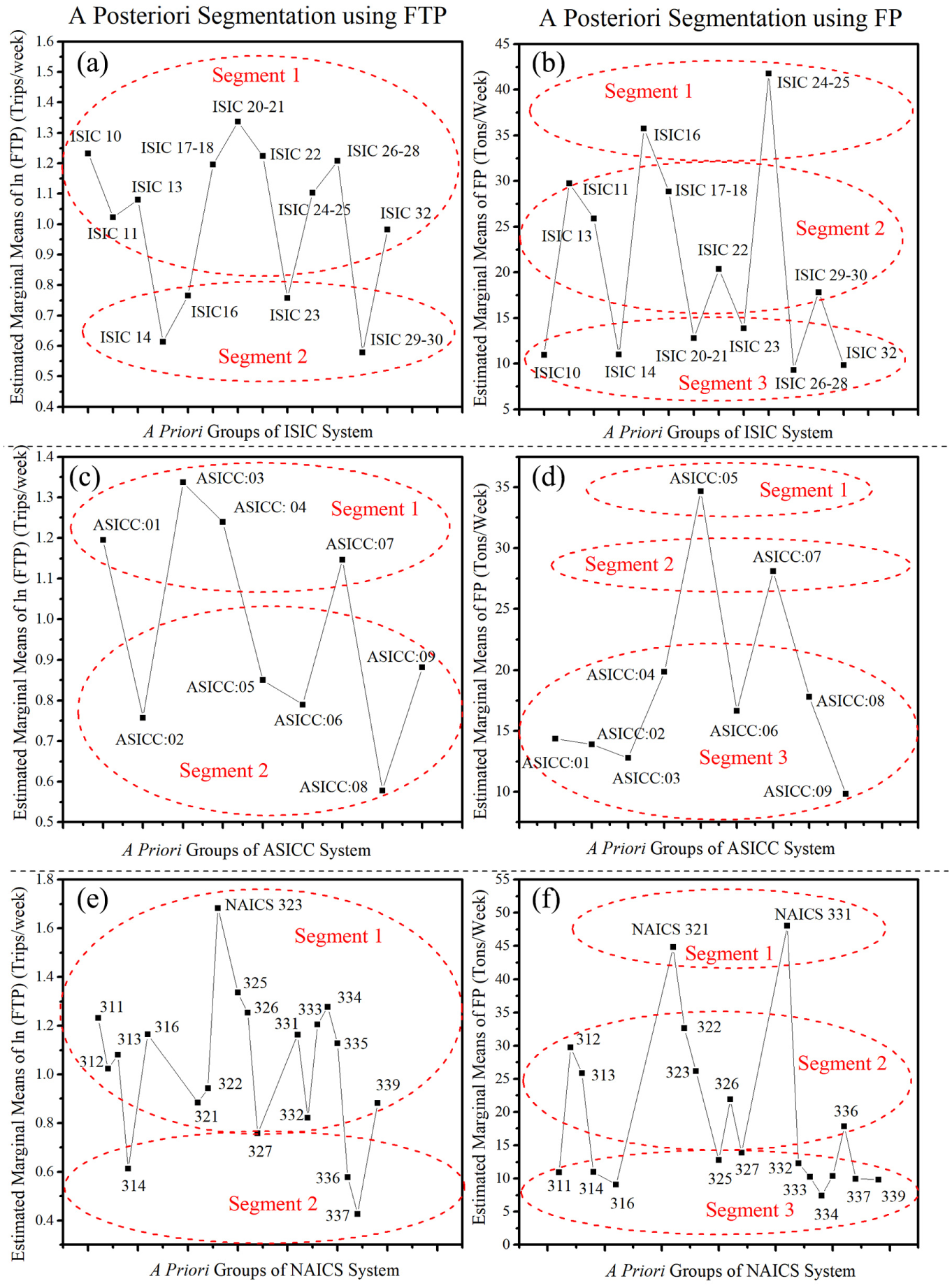
Marginal means plots for a posteriori segmentation using FTP and FP characteristics: (a) ISIC FTP, (b) ISIC FP, (c) ASICC FTP, (d) ASICC FP, (e) NAICS FTP, (f) NAICS FP.
ASICC-Based Segmentation
The analyses were repeated for data coded using the ASICC system. The significant value for Levene’s test statistic led to taking natural logarithmic transformation for variance stabilization. The subsequent Levene’s test revealed a test statistic of 0.527 (significance = 0.836) which suggested that ANOVA procedure can be applied. Pair-wise LSD test comparisons were carried out analogous to ISIC-based segmentation and the ASICC classes led to two FTP segments and three FP segments. The divisions and marginal means of ASICC are given in Figure 2c and 2d.
NAICS-Based Segmentation
The analyses were repeated for NAICS segmentation using FTP and FP patterns. The segment divisions based on LSD test and the corresponding marginal means of appended NAICS groups are given in Figure 2e and 2f. Despite having 19 NAICS groups, LSD test led to two FTP segments and three FP segments, much like the case of ISIC-based and ASICC-based segmentation.
A Posteriori Segmentation Based on SS
A closer look at FP and FTP segments revealed that the industrial classes (e.g., ISIC:10, ISIC:11, ISIC:20–21) appended in segments with high marginal mean of FTP (three to four trips/week) typically correspond to segments with low or medium marginal mean of FP (8 to 30 tons/week). With few exceptions, this inverse correspondence recurs in the case of both NAICS and ASICC segmentations as well. This dichotomy observed between a posteriori segments corroborates the empirical evidence and discussions provided by Tavasszy and De Jong ( 5 ) and Holguín-Veras et al. ( 1 ) regarding the underlying influence of logistical decisions on distinguishing FTP and FP. That is, an increase in FTP may not necessarily result in an increase in FP due to flexibility in choosing SS. The role of SS is latent here because establishments in each industrial class could differentially increase FTP, without increasing FP, by merely decreasing SS, and in turn, changing the type (and size) of vehicle used for transporting goods. Due to the indivisibility of truck trips, transporting small shipments constitutes the same number of truck trips as a large one. In essence, flexibilities in SS enable industrial classes with high FTP to generate lower FP than those industry classes with low FTP. The converse corollary (i.e., high FP segment corresponding to low FTP segment) does not hold true for most of the industrial classes, bowever,. Instead, industrial classes with high FP values (e.g., ISIC:24–25, NAICS:321) are mostly found with high FTP values. Likewise, industrial classes with low FTP values (e.g., ISIC:23, NAICS:314, ASICC:06) are typically characterized by low FP values.
In order to assess the latent effect of SS and its implications for modeling FP and FTP, a posteriori segmentation using SS was subsequently carried out. The pair-wise comparisons using LSD test led to five segments in the case of ISIC classes and NAICS classes, whereas four segments were revealed in the case of ASICC classes. The segment divisions and marginal means of industrial classes are presented in Figure 3. The a posteriori segmentation results reveal that industrial classes (e.g., ISIC:20–21, ISIC:10) appended in segments with high FTP (four trips/week) correspond to SS segments with low or medium SS (1 to 7 tons/trip). This inverse correspondence substantiates the hypothesized latent effect of SS in distinguishing FP and FTP. The industrial classes in FP segments and SS segments, on the other hand, as expected share a direct correspondence. For instance, industrial classes (ISIC:27, ISIC:24–25) placed in segments with high marginal mean of FP (36 to 41 tons/week) correspond to segments with high marginal mean of SS, such as segment 1 (19 tons/shipment) or segment 2 (17 tons/shipment). Overall, the contrasts and parallels drawn between a posteriori segments illustrate the following: (i) the importance of distinguishing FP and FTP when estimating freight movements; (ii) the importance of capturing the underlying influence of logistical decisions when estimating FP and FTP; and (iii) the potential of using variations SS for grouping industrial classes when categorizing and aggregating freight data.
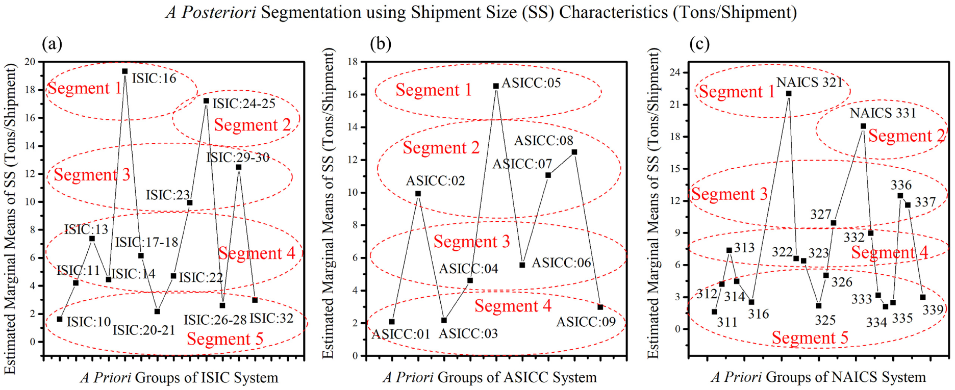
Marginal means plots for a posteriori segmentation based on SS characteristics: (a) ISIC, (b) ASICC, (c) NAICS.
Relationship between A Posteriori Segments and Commodity Value Density
Based on a posteriori segment membership of each establishment, EBFS data was analyzed using commodity value density (value per 1 kg) to provide useful interpretations and identifiable traits for each segment. The mean FTP, FP, and SS of each segment was compared against its mean value density, as shown in Figure 4. In the case of FP and SS segments, it may be noted that ISIC and NAICS have largely similar variation in terms of value density. This could be due to the similarities in codal structure; ASICC segments are visibly distinct from the segments based on other classification systems. As the value density of commodity handled by the industrial class increases, FTP also increases. In contrast, an increase in value density corresponds to a decrease in FP and SS of segments. This reflects, of course, the inveterate truism that high-value commodities are transported in smaller and, in turn, more frequent, shipments to save inventory holding costs ( 22 ). Another reason could be that the amounts of capital and opportunity costs tied up with these commodities while in transit are high, therefore they tend to be released in small shipments as soon as possible. This pattern is not true for ASICC-based segments, however, since they show non-monotonic variation with respect to value density. It is expected that the interpretations of value density traits of proposed a posteriori segments will be helpful for considering them as a base for future freight data collection plans and subsequent development of FG/FTG models.
Identifiable traits of a posteriori segments in terms of commodity value density: (a) FTP, (b) FP, (c) SS.
Comparative Assessment of Model Performance of Various Segmentation Schemes
This analysis aims to quantify the extent of variability in FTP and FP across establishments grouped using different classifications. Two-level hierarchical linear models were estimated to partition the variability in FTP and FP which could be attributed to industrial classifications (level 2) and to establishments within those classifications (level 1). The models included employment, the traditional business size predictor, as a covariate. Restricted maximum likelihood estimates were obtained for FTP and FP. Firstly, unconstrained null models were estimated to assess the variation between industrial classes as a proportion of the total variance. The results of ICC are given in Table 5A. Goodness-of-fit of null models were calculated using Akaike information criterion (AIC), with smaller values indicating a better fit. The results indicate that the proportion of variance attributable to industrial classification systems varies between 1.1% and 50.7%. For instance, an ICC of 0.426 in the case of ISIC-based a priori industrial classes reveals that 42.6% of the total variation in outcome occurs between ISIC classes. It may be seen that the difference between FTP patterns of NAICS classes amounts to 38.7% and for ASICC classes it amounts to 35.2%. In the case of FP, NAICS codes are found to amount to 31.6% of total variation across establishments, as opposed to 23.4% explained by ISIC and 11.8% explained by ASICC. These findings illustrate that the alternative classification systems are likely to have a substantial effect on the estimates for FP and FTP.
A. Variability in FP and FTP across Segmentation Schemes, and B. Performance of Employment-based FP and FTP Models across Segmentation Schemes
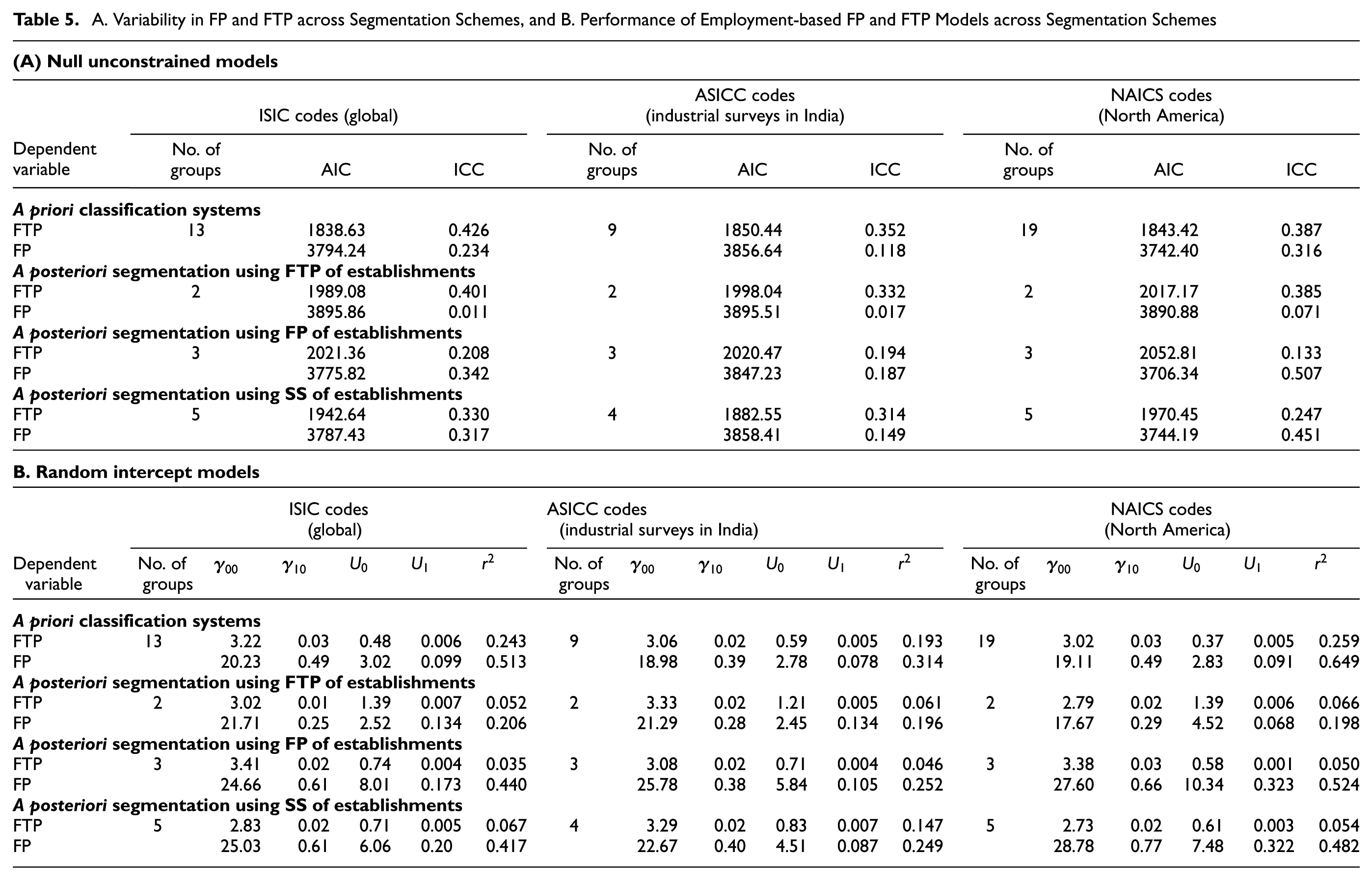
The random intercept models were subsequently estimated to assess the variation in the relationship between FP or FTP and employment across different classification systems. The model estimation results are presented in Table 5B. The significance of HLM coefficients confirms the relationship between employment and FP/FTP. The variance explained by employment in FP/FTP is given by r 2 values. For instance, the r 2 value of 0.513 in the case of ISIC-based a priori classes indicates that employment explains 51.3% of variance in FP when establishments are grouped by ISIC codes. It is apparent that the predictive ability of employment varies considerably across alternative classification systems, as illustrated in Figure 5. Comparison of r 2 values reveals that NAICS performs better for estimating FP. This finding is confirmed by a posteriori segments based on NAICS codes as well. In the case of FTP, model estimation results confirm the findings of Sánchez-Díaz ( 8 ) and Gonzalez-Feliu ( 7 ) on FTA that a considerable portion of the variability in freight trips arises independently of the classification systems. This may be explained in terms of another finding in this paper, that FTP is the result of logistical decisions of establishments which hinge on the choice of SS. This reasoning is substantiated further in the FTP model estimation results since models using SS segments offer better prediction accuracy.
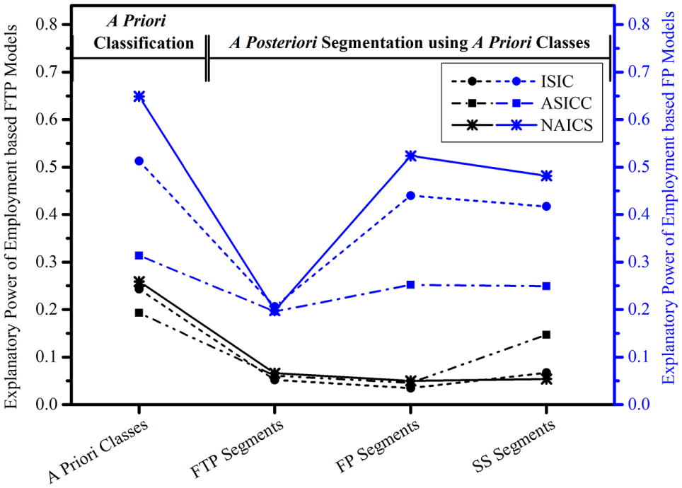
Comparison of model performance for different classification systems.
The model estimation results also reveal that a posteriori segmentation schemes perform reasonably well in comparison to a priori classification systems, despite having significantly smaller numbers of groups. This is particularly relevant for FP models since the explanatory powers using both the segmentation schemes are comparable, when SS size is considered in a posteriori segmentation. However, it may be noted that FP segments are limited in their explanatory power for predicting FTP, and vice versa. The explanatory power of SS segments is better than the other two types of segments for predicting FP as well as FTP. Given the need to develop FP and FTP models using the same classification systems for comparability, SS segments may thus represent an acceptable middle ground for freight demand modeling.
Conclusion
This paper contributes to the understanding of industrial classification systems for modeling freight demand. It begins by providing a systematic overview of different a priori industrial classification systems, underlying linkages in codal structure and classification approach used in freight studies around the world. The classification systems considered for analysis are NAICS, ISIC, and ASICC. Based on the a priori industrial classes, a posteriori segments are developed by ordering and appending industrial classes which do not have statistically significant differences in LSD test. Regardless of the classification systems, LSD tests led to two FTP and three FP segments. The dichotomy between industrial classes appended in FTP and FP segments clearly revealed the latent influence of SS in distinguishing FTP and FP. Segmentation by SS led to five segments in the case of ISIC and NAICS, whereas for ASICC it led to four segments. Overall comparison showed that industrial classes in FP and SS segments have direct correspondence. In contrast, industrial classes in FTP and SS segments have inverse correspondence. These findings are in line with the general consensus regarding the underlying influence of SS when estimating FP and FTP. Analyzing the commodity value density of a posteriori segments showed that industrial classes handling commodities of high value density tend to have low FTP, high FP, and high SS. This may be explained using the popular assertion that high-value products are transported in smaller and more frequent shipments to save inventory holding costs and amount of capital tied up in a single shipment.
The paper also compares the performance of a priori and a posteriori segmentation schemes in modeling FTP and FP. The two-level hierarchical linear FP models revealed that industrial classification systems (NAICS, ISIC) perform significantly better than a product classification system (ASICC). This is logically appropriate since freight movements are derived from economic activities and thus defining establishment groups by economic activity should result in improved model predictions. The implication of this finding is that we can have greater confidence in the model systems provided by existing studies which have used NAICS- or ISIC-based classification systems to group establishments. Another implication is that it points towards the importance of adopting ISIC-based classification systems for modeling FP in countries outside of North America (e.g., NIC in India, SBI in the Netherlands, KSIC in Korea, NAF in France, SNI in Sweden), rather than relying upon country-specific indigenous classification systems such as ASICC. Adopting such classifications based on a global reference is crucial for improving the comparability of freight studies conducted around the world. In the case of FTP, however, a considerable portion of variability does not depend on the number of employees, regardless of the classification systems, whether NAICS or ISIC. This finding underlines the general consensus that vehicle-based FTP models are largely influenced by logistical decisions hinging on size of shipments, unlike commodity-based FP models. The model estimation results also suggest that a posteriori segmentation schemes—especially using SS—are comparable with those of a priori classification systems, with the advantage of having significantly smaller numbers of groups. This finding illustrates the potential of a posteriori segmentation for saving time and cost in future freight planning surveys and consequently reducing the sample size implications of having to develop numerous planning models. The resultant segments are novel yet meaningful subgroups of the freight travel market with homogeneous freight travel patterns (FTP/FP/SS). FP/FTP models estimated using these segmentation schemes maintain their applicability to external data still stored in a priori classes (e.g., NAICS employment statistics). The model comparisons between these segments reveal that FTP segments are limited in their explanatory power for predicting FP, and vice versa. The SS a posteriori segments may represent an effective middle ground for developing FP/FTP models in freight demand model systems. Overall, the study findings are expected to assist research efforts to improve freight data segmentation across the world so that it corresponds to modern logistic structures in a highly urbanized world.
Footnotes
Author Contributions
The authors confirm contribution to the paper as follows: study conception and design: P. K. Sahu and A. Pani; data collection: A. Pani; analysis and interpretation of results: A. Pani and P. K. Sahu; draft manuscript preparation and correction: A. Pani and P. K. Sahu. Both authors reviewed the results and approved the final version of the manuscript.
The Standing Committee on Freight Transportation Planning and Logistics (AT015) peer-reviewed this paper (19-02465).