
Abstract
There is a huge potential for exploiting information centered on individual transit users’ behavior through longitudinal smart card data. This is particularly true for cities like Gatineau, Canada, where the bus system serves passengers with different travel patterns. Understanding the evolution of these patterns marks an important point in improving transit demand forecasting models. Indeed, better models can help transit planners to create optimized networks. This paper proposes a comparison of a traditional and an experimental methodology aiming to identify the evolution of travel structure among transit users. These methodologies are based on the clustering of multi-week travel patterns derived from a large sample of smart card transactions (35.4 million). Representing users’ behavior, these patterns are constructed using the number of trips made by every card on each day of a week. Behavior vectors are defined by seven components (one for each day) and are clustered using a K-means algorithm. The experimental week-to-week method consists in clustering the population on each week, while using the clustering results from the previous week as seed. This latter approach makes it possible to observe the evolution of users’ behaviors and also has a better clustering quality in a similar computation time than the traditional method.
To limit negative impacts of rapid urbanization, public transit systems have been adopted worldwide to help reduce traffic congestion. Hence, for several decades, most of the cities in the world have developed transit networks based on demand. A common phenomenon stands out in many metropolitan cities; the demand is evolving and this variation of ridership triggers various problems like overcrowding in public transportation ( 1 ). Customer loyalty models clearly show that overcrowding is a critical attribute for transit usage ( 2 ). Thus, there is an increasing need to provide a better understanding of demand, especially looking at its evolution over time, helping to match transit services in the context of limited resources.
Traditionally, planners have used travel surveys (household travel survey, on-board surveys, etc.) to analyze transit use. According to the fullness of their information, planners were able to carry out some statistical studies about the network and estimate demand with a good accuracy. In view of their cost, however, these surveys could not be conducted frequently, which meant that the temporal variations in user behaviors could not be assessed easily.
Thus, a way to gain cheaper and more accurate analysis of transit users’ behavior arose. Emerging technologies allow planners to work with smart card data fare collection systems. These systems generate anonymized ticketing data on transit usage and can be used to implement new modeling approaches for urban mobility analyses. The data has the advantages of being spatially and temporally precise, however, as they do not need to ask users question in order to collect data, they are not linked to survey information like socioeconomic data or trip purpose. Furthermore, the huge amount of data collected in large cities raises several challenges and computing issues.
Since around 2010, many researchers have worked on these challenges, particularly on understanding users’ habits. Finding mobility patterns through clustering approaches helps to create realistic models of the network and thence forecast passenger behaviors. Many methods have been developed to identify these patterns; some of them are described in the related work section. These researches seldom look at the evolution of such patterns over time, however. The aim of this paper is to propose a weekly-based analysis of users’ behaviors. A comparison between a traditional and an experimental clustering method is provided, based on smart card data collected over a long period of time.
This paper makes the following contributions:
All card holders are analyzed through their weekly activities. Their behaviors, represented by a vector counting the number of trips made each day of the week, are clustered to find similarities among groups of users.
The paper exploits an experimental technique to show that transit users’ behaviors change over time, so a temporally fixed representation of the population is not adequate.
Clustering quality and stability indicators are used to show the differences between the methods and to qualify the population behaviors.
This article is organized as follows. In the next section, some background from the literature about smart card data and its applications in the public transportation industry is presented. In the third section, the methodology and the case study are presented. The experiments were conducted using a dataset from the smart card automated fare collection (SCAFC) system of a small Canadian transit authority. The findings are summarized, with the contributions of this study, its limitiations, and future work, in the concluding section.
Related Work
Smart card data stands out among the different types of data source used to analyze transit user behaviors ( 3 ). It is one of the most complete sources, thanks to the traceability of every (anonymized) card. At each use of the network, every transaction is timestamped and geotagged, creating a massive volume of data. The challenge of analyzing such big data sets is accompanied by the incompleteness of some information (particularly trip destination) and the lack of socioeconomic data. As documented by Pelletier et al. ( 4 ), however, many authors have shown an interest in this matter and developed several tools for data mining and results analysis in transportation, for renovating traditional travel behavior research.
The potential of smart card data for transit planning was originally introduced by Bagchi and White ( 5 , 6 ). They analyzed three cities in the United Kingdom using rule-based processing on bus transactions to estimate trip rates and the proportion of linked trips. Subsequently, various analyses were applied all around the world. Devillaine et al. ( 7 ) worked on an activity model using smart card data from Santiago in Chile and Gatineau in Canada. They established different rules to detect an activity based on trip routes and time gap between transactions, and then compared the behavioral activity patterns between these cities. Goulet-Langlois et al. ( 8 ) developed a method based on clustering similar multi-week activity sequences in London. These activities are defined by areas, and so going to another area is like doing a different activity. Regarding the sequences, they analyzed the heterogeneity among the passengers. Additionally, they experimented with a cluster stability study and a cross-analysis with socio-demographic data on their result.
Aiming to solve the issue of the lack of information about destinations through smart card usage, many researchers have proposed some method to estimate the alighting stops. For example, Barry et al. ( 9 ) proposed a rule-based method to estimate destinations in the New York City subway. Indeed, these authors established that, after each trip, users will return to the previous station to go somewhere else and that at the end of the day, users will return to the station where they first boarded the same day. To improve this method, Trépanier et al. ( 10 ) added a distance-based rule about the next boarding and the possibility of looking at the weekly travel patterns to fulfill missing alighting information. More recently, Alsger et al. ( 11 ) evaluated common trip-chaining assumptions on SCAFC in Queensland, Australia. A special feature of these data is that they have alighting information, so the authors decided to estimate destinations and compare their estimates with the real ones.
Understanding transit users’ behaviors represents one the main challenge in smart card data analysis. Mahrsi et al. ( 12 ) developed an approach helping transit planners to understand the demand, testing their method on the bus and subway system in Rennes, France. They decided to cluster similar temporal behaviors based on boarding time, and to study the effect of distribution of socioeconomic characteristics. In the literature, the majority of the studies on transit users’ behaviors focus on the repeatability of temporal activities, but some have proposed to cluster spatial and temporal patterns. Ma et al. ( 13 ), for example, developed a spatial and temporal approach using a density-based clustering algorithm. Using a K-means++ algorithm, they were also able to identify travel regularity. Trépanier and Morency ( 14 ) developed this notion of travel loyalty in behavior analysis, analyzing rider retention and identifying behaviors by smart card fair type.
Engineers have been working on forecasting data for many years. In transportation, they traditionally focused on flow forecasting to estimate required infrastructure capacities. Techniques have differed, and recently some have begun to use emerging technologies. For instance, Ni et al. ( 15 ) used social media data from Twitter to explain and forecast real-time passenger flow using seasonal ARIMA models. The ARMA approach ( 16 ) and its variants (ARIMA, SARIMA) has also attracted a lot of attention by researchers. These methods make it possible to solve some issues in time series but they retain the disadvantages of inability to make long-term forecasts or to detect special events. Li et al. ( 17 ) focused on this challenge of forecasting disruptions caused by special events. Indeed, non-regular passenger demands are very difficult to determine through conventional methods, which is why that study proposed a novel class of multiscale radial basis function to represent the underlying dynamics of the abnormal Beijing subway network. Leng et al. ( 18 ) developed a method through a probability tree created by learning the probability of each kind of historical origin–destination pair in the Beijing subway system. This tree can be updated in order to acquire real-time comprehensive information on passenger flows in stations. Interested by flow forecasts of subway transfer stations, Sun et al. ( 19 ) developed a nonparametric regression model with a one-month training base to calibrate the algorithm. Their results show that the method makes it possible to estimate passenger flows in transfer stations with greater accuracy than traditional methods.
Other authors have worked on behaviors and ways to forecast users’ habits. For instance, Foell et al. ( 20 ) described a generic pattern mining approach to estimate mobility behaviors, evaluating bus ridership data. This method defines four independent features describing discriminative properties of users’ behaviors on travel histories and uses a naïve Bayes classifier to capture these behaviors.
Methodology
This section presents the proposed methodology. A comparison of two clustering techniques is made to group transit users based on their behaviors recorded by a SCAFC system: a traditional K-means clustering technique and an experimental week-to-week K-means clustering technique. The different algorithms are applied following the method explained in the SADT diagram (Figure 1).
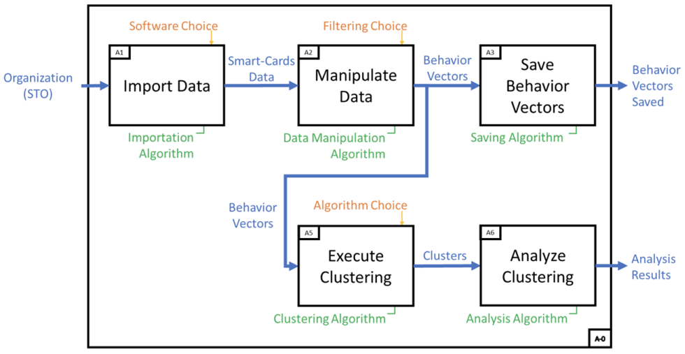
Methodology steps.
Data Manipulation
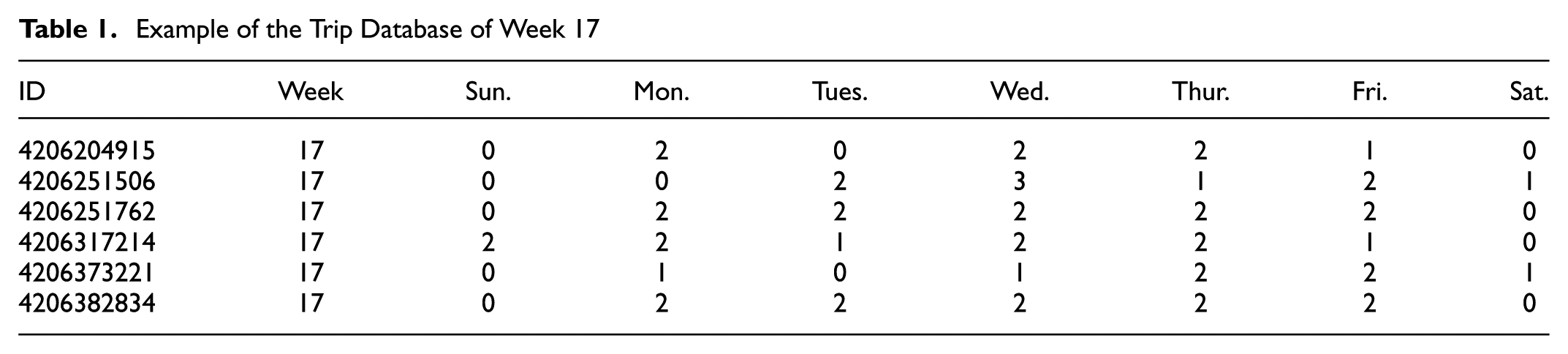
First, the smart card transaction database is cleaned and transformed into a trip database, creating trip tables for every week of the study period (Table 1) and describing the behavior of each card. Each column represents a day of the week (from Monday to Sunday) and each record represents the number of trips completed each day of the week by a card. These records will be named “behavior vectors” and represent non-stationary temporal data. These vectors are intentionally made simple to illustrate the relevance of the methods and represent the input data for the clustering.
Example of the Trip Database of Week 17
Traditional K-Means Clustering
Clustering constitutes the main organ in this study, it allows us to regroup users based on the similarity of their behaviors. K-means is one of the simplest and fastest distance-based algorithms in big data clustering. Introduced by McQueen ( 21 ) and presented in Figure 2, the algorithm has the disadvantage of being very dependent on its initialization. Indeed, it usually converges to a local optimum instead of finding the best one.
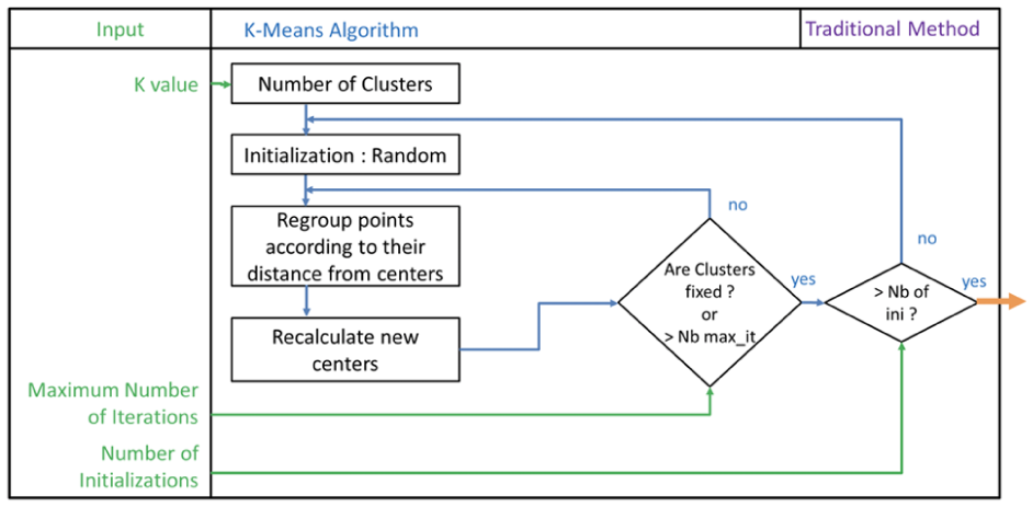
The K-means algorithm.
The algorithm needs some inputs to work, such as, for example, the choice of the number of clusters: K. Often chosen totally arbitrarily, this choice regularly leads to discussion. Naturally, too many clusters will make the analysis too detailed, losing the purpose of clustering, while too few clusters will not produce enough information to characterize the population. Thus, numerous indicators have been developed to help the analyst to optimize the choice of the K value. The literature generally refers to the elbow method developed by Thorndike ( 22 ), the silhouette method introduced by Rousseeuw ( 23 ), and the gap method by Tibshirani et al. ( 24 ). Presenting some issues of computer resources and time completion, the dendrogram method explained by Morency et al. ( 25 ) is preferred. This method consists in simulating a K-means clustering on all data with a high number of clusters, and to compute the results into hierarchical agglomerative clustering (HAC) to observe the data distribution better. To optimize the K value, this study proposes an arbitrary choice based on the distortion level of merging clusters. The maximum number of iterations and the number of initializations represent the two remaining parameters of the algorithm. Specifying a higher value for these parameters gives a better clustering quality in spite of a longer computation time. Indeed, the maximum number of iteration forces the algorithm to give results in cases where convergence does not appear, and the number of initializations indicates how many times the loop must be done before giving the best results.
The initialization consists in giving a set of K randomly generated centers to the grouping step. As it represents the main limitation of the method, some authors have taken an interest in improving the initialization step. The best-known enhancement of the K-means algorithm is the K-means++algorithm proposed by Arthur et al. ( 26 ). It generates optimized cores after each iteration and inputs these cores to the next iteration instead of using random initialization. Hence, the algorithm provides better quality results usually with a faster convergence.
The traditional method first regroups the trip tables into one and then runs the K-means algorithm on all the data. Thus, the algorithm provides K clusters, defined by their center, which is the barycenter of all points in the cluster. Every behavior vector gets the information of the cluster it belongs to. This way, the method makes it possible to show the evolution of the different clusters population, helping planners to understand user demand better. Performing best on short periods, the traditional method is mostly applied to compare the same week in different years ( 27 ).
Experimental Week-to-Week K-Means Clustering
Following the hypothesis that progressive tampering allows evolution of clusters through time ( 28 ), this study proposes an experimental clustering technique based on K-means. Indeed, this algorithm aims to get faster and higher clustering quality than the traditional method, through a temporal partitioning of the data.
The algorithm, explained in Figure 3, consists in incrementally running K-means on each week of the study period, in chronological order. The s week will be clustered by forcing the input of previous results (s-1, s-2, …, 1) as new cores. Cores are defined as the centers originally input in initializations. On each iteration, the method applies a training function on these previous results to get a unique set of K cores. Thus, the algorithm needs an initialization, consisting in running the traditional clustering technique on at least one year of data. Results of this process are used as a training base and are inputted as K-means cores for the first week simulated.
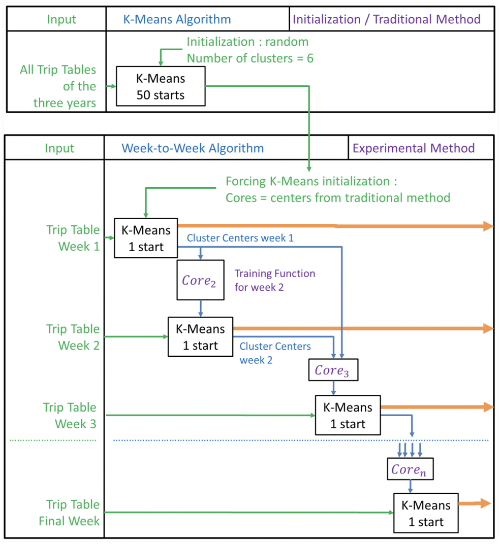
The experimental week-to-week K-means clustering.
It is necessary to identify holiday weeks as a week with at least one public holiday or school break, because it is common to notice a decrease of 80% of ridership on these weeks. This experimental method is sufficiently dependent on the previous weeks to be skewed by a holiday week. Some weeks are reported to be declining due to the presence of public holidays, but the training function is dimensioned to solve this issue. This training function can be written as:
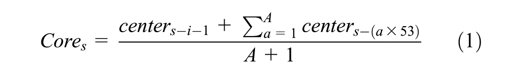
where
The experimental method works on a weekly partitioned data and defines K clusters for each week. The training function allows the algorithm to follow each cluster through time, and so the evolution of their center. This way, a behavior evolution analysis is possible, helping planners to gain more information about the users’ demand.
Analysis
The center of a cluster matches the mean number of trips users (of the same group) did on each day of the week. The experimental method allows the evolution of the centers through time, while the traditional method considers them stationary. Analyzing this evolution is interesting to understand users’ behaviors better. When working on regular fare types, interpretability of daily transit usage usually provides a good approximation of the population.
The multiplication of the population and the number of trips on each day will give the transit planners the number of trips taken by the population of this cluster. As the evolution of the population in groups is usually seasonal, its analysis could be a great opportunity to get a better understanding of the evolution of network usage.
In clustering, data analysts are looking for the best between-cluster heterogeneity and within-cluster homogeneity. Thus, the Dunn criterion D is chosen ( 29 ) to qualify the clustering quality, in order to maximize between-cluster distances and minimize within-cluster distances. It can be written as:

In Equation 2, i, j, and k represent clusters, d(i,j) represents the Euclidean distance between centers of cluster i and j, while d’(k) represents the sum of Euclidean distances between each element in the cluster k and the center of the cluster. The higher the indicator value, the better the clustering quality will be.
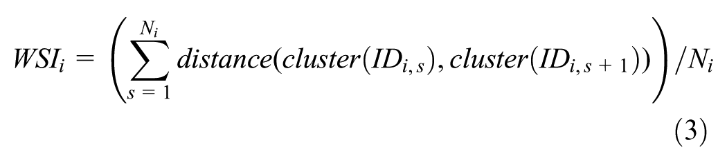
In transit planning, planners are looking for tools to characterize behavior changes. In that respect, Leskovec (
30
) developed a weight sequential instability (WSI) indicator to qualify users’ behaviors. This indicator focuses on the distance users travel between clusters through time and is equal to the sum of the Euclidean distances between centers of successive clusters visited by a card, divided by the number of weeks traveled
Case Study
This section presents the different results and analysis of the proposed methodology in our case study. It compares both clustering methods on three criteria: computation speed, quality, and users’ stability, however, only the three most interesting clusters will be presented here.
Transit Authority
The Société de Transport de l’Outaouais (STO) is a medium-size public transport authority in Gatineau, Québec, Canada, operating since 1971. STO introduced a smart card fare system in 2001, and today in 2018 more than 80% of STO passengers use Multi, the smart card providing access to the service. Every STO bus is equipped with a GPS reader, storing data about location and timestamp when a user boards. Protection of users’ privacy is important; thus, every card is anonymized. Gatineau is an extended city across Ontario River and close to the capital of Canada, Ottawa, and its 934,243 inhabitants (according to the 2016 census). Consequently, there are many STO buses connecting both cities. The activities of these travelers are particularly work related. In October 2013, STO introduced Rapibus, a bus rapid transit system using bus-designated lanes alleviating the main arteries and connecting with Ottawa, a popular work destination.
Information System
For this study, transactions from bus usage in Gatineau provided by STO from January 2012 to December 2014 were used. Each transaction includes information about users (anonymized card ID, type of transit fare), transaction (stop number, day, hour, and if it is a transfer or not) and the chosen bus line (time of departure, direction, service, line, and bus number). After standard cleaning, only regular adult transit fares are kept for further analysis. Thus, 28.2 million transactions were made during this period by more than 44,077 cards. Many cards, mostly with student fares, are reprinted and anonymized every year, so the number of cards is not useful and a year-to-year user behavior cannot be applied for these users. For more relevancy, the transactions must be transformed into trips; thus users made 9.6 million trips in three years. Finally, the algorithm created 1.25 million vectors of behaviors from card_id and timestamp, following the previously described methodology.
Choosing the Number of Clusters
The traditional K-means clustering works on all temporal data, and so it will be computed on all the merged trip tables. To determine the optimal K value, HAC is computed on the centers of the 30 clusters obtained by a K-means clustering on all the data. According to the following dendrogram, an arbitrary choice of K = 6 is made due to the data repartition and the dissimilarity of merging clusters (Figure 4).
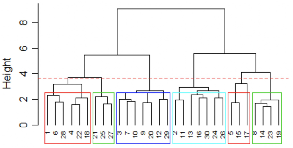
Dendrogram, the K-choice method application.
Clustering
The traditional K-means clustering algorithm is computed on the three years of data (159 weeks) with a K value of 6. Some other parameters are requested: the number of random starts is fixed to 50 and the maximum number of iterations to 100. These parameters were arbitrarily chosen high to maximize the chance of a conversion to the optimum, despite the time of computation.
For the experimental method, the algorithm begins with an initialization on at least one year of data. To get the best performances, the initialization is here computed on the three years of data. The algorithm then recovers the different information from previous weeks and the actual week trip table, to cluster the population on the actual week. The K-means algorithm is therefore computed on smaller datasets, and so gets a faster convergence. This way, clusters centers are not the same along the weeks allowing to capture evolution.
Analysis
The analysis work begins with the study of the clustering results. From a quantitative viewpoint, the cluster 2 travelers are doing two trips on each day of the week and no trip on weekends (Figure 5). The cluster 2 population represents an average of 28.6% of the regular cards on each week and follows a positive trend with seasonality. Indeed, the population graph shows decreases during summer and increases in working periods. This cluster is also extremely dependent on holiday weeks because its population fully disappears on these weeks. Hence, this group seems to contain a population of regular workers or students who generally follow these different parameters. From a comparative viewpoint, both methods provide similar results except on holiday weeks. The experimental method seems to follow the users’ behaviors better, increasing trips on weekends and decreasing trips on days of the week in holiday weeks.
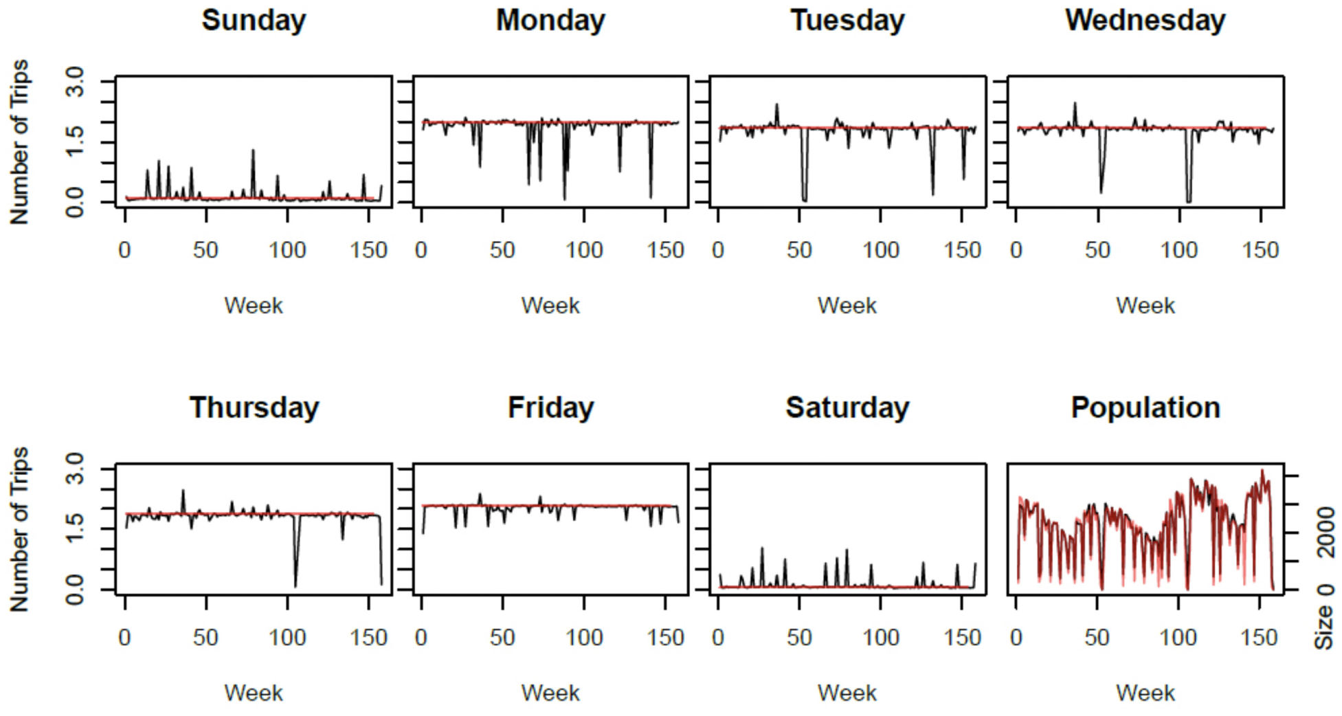
Centers and population evolution in cluster 2: red = traditional, black = experimental.
In contrast, the cluster 1 analysis provides a different interpretation (Figure 6). The group population only travels on week days except on Mondays, doing round trips. This population represents 18.5% of the regular cards and appears to be constant with a slight seasonality along the years. This group also seems to recover the cluster 2 population on holiday weeks, probably because public holidays are often on Mondays in Canada. So, this cluster could contain a population of workers who do not work on Mondays and recover regular workers on public holidays. In the method comparison, some differences appear, particularly on Tuesdays and Fridays, where the experimental method shows an evolution of transit usage. Usage on Fridays seems to follow seasonality and distinctly shows a decrease on the Easter weekend of each year. On Tuesdays, the curve clearly shows the three years with an increase of transport usage in the second year (average of two trips per user) followed by a decrease on the third one (average of one trip per user). This change in users’ behaviors is an opportunity for transit planners to find a connection with a 2014 network change.
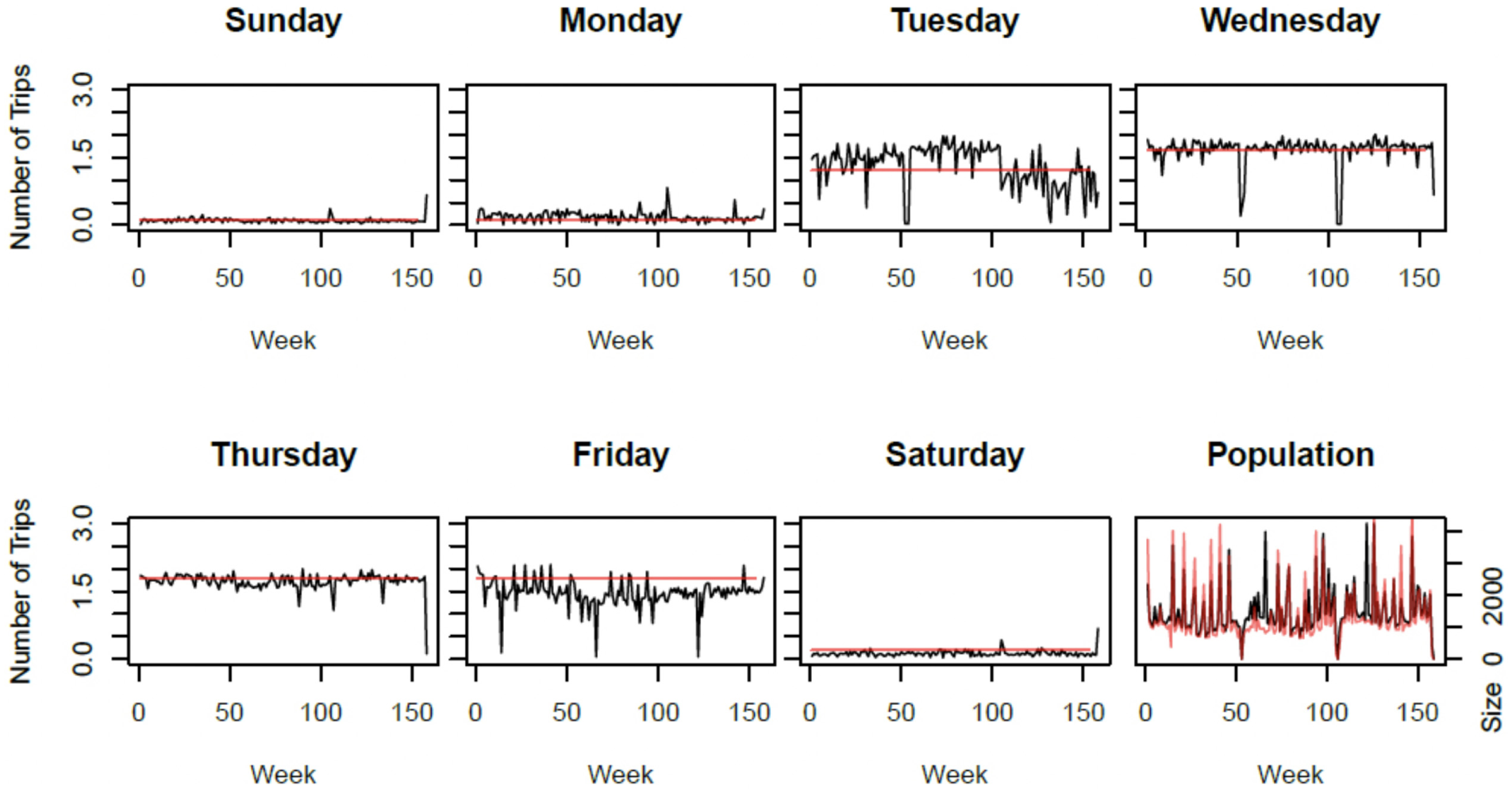
Centers and population evolution in cluster 1: red: traditional method, black: experimental method.
From a quantitative viewpoint, cluster 5 seems to contain the population which generates the most trips (Figure 7). These travelers are making an average of two trips per day, and one on Sundays. This population represents 12% of the regular cards and is constant along the years. There is no influence of holiday weeks on transit usage in this cluster, except in the Christmas period. This cluster could thus contain non-workers who are familiar with daily trips. From a comparative viewpoint, both methods provide similar results, the experimental one seems to show more trips on week days than the traditional method. The average number of trips on week days are following the same trends, showing the influence of external events like weather, which is a significant factor in transit planning in Canada.
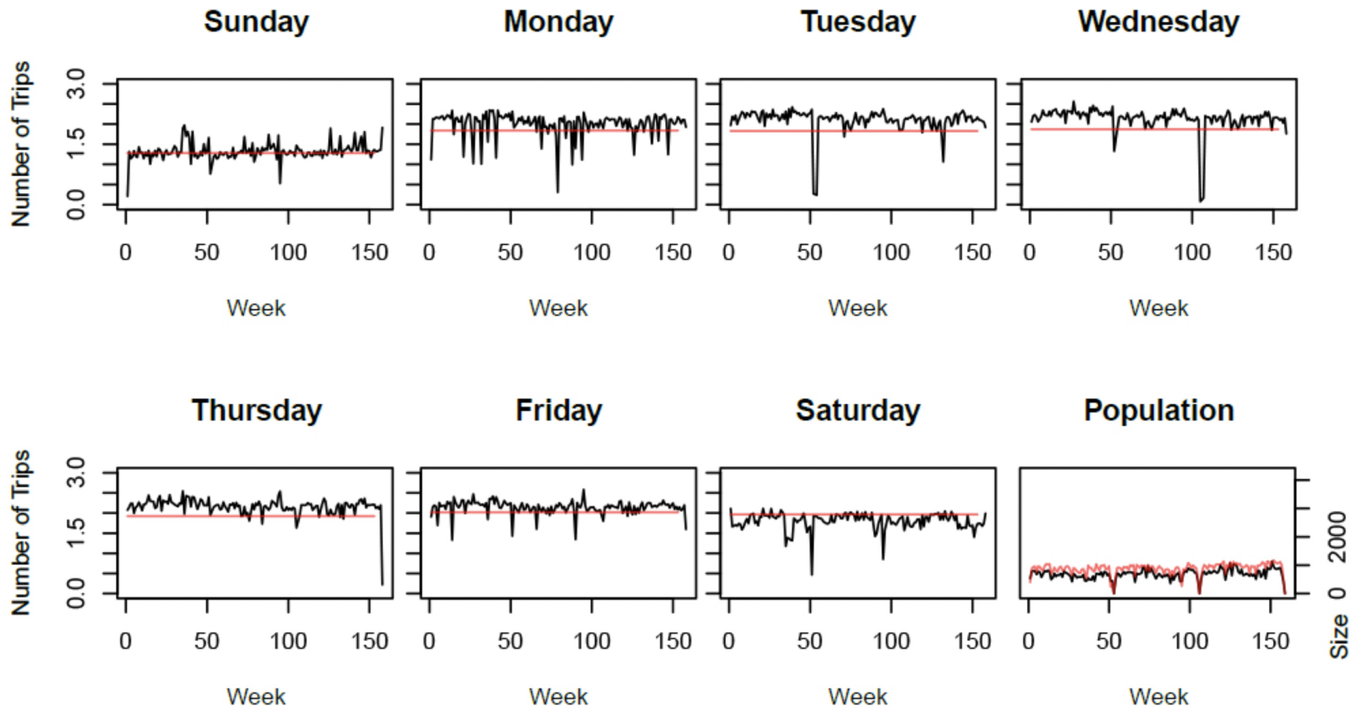
Centers and population evolution in cluster 5: red: traditional method, black: experimental method.
The analysis continues with the evaluation of the clustering quality. The algorithm calculates the Dunn criterion for each week of the study period for both algorithms. Recalling that the higher the criterion value, the better the clustering quality will be, the results are presented on Figure 8 illustrating the comparison of these methods. The traditional method shows real quality issues on holiday weeks, unlike the experimental method which performs better on these. Figure 8a presents seasonality, which seems to be inversely proportional to the transit ridership, and Figure 8b shows that the Dunn criterion of the experimental method is, most of the time, higher than the traditional one.
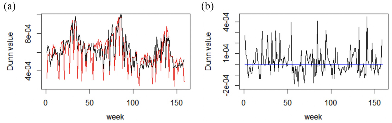
Dunn criterion comparison: (a) evolution of the Dunn criterion for the experimental method (black) and the traditional method (red) and (b) evolution of the difference of these methods.
Qualifying users’ behaviors often leads to discussion. Here, a WSI criterion is calculated for all individual transit cards. As explained in the methodology, a low WSI value indicates a good stability, meaning that the user is not changing clusters that much over time. Figure 9 shows the distribution of the WSI values of the users who made more than four trips. For both methods, there is approximately 12% of the population with a WSI value below 1; they are considered as stable users who only travel between close clusters or not at all, meaning that they hardly ever change their behaviors. Most of the population, with a WSI value included between 1 and 2, have an evolving behavior week after week, increasing or decreasing the number of trips according to the season. Those with a 2+ WSI value, representing less than 10% of the population, have an unbalanced behavior: they rarely replicate the same pattern along the weeks. According to the fact that the box diagrams do not follow a normal distribution, a Wilcoxon test must be computed to compare these samples. The test gave the traditional method greater instability than the experimental, and so confirmed that users travel less between clusters with the experimental method. Therefore, the latter seems to follow the users’ behaviors better.
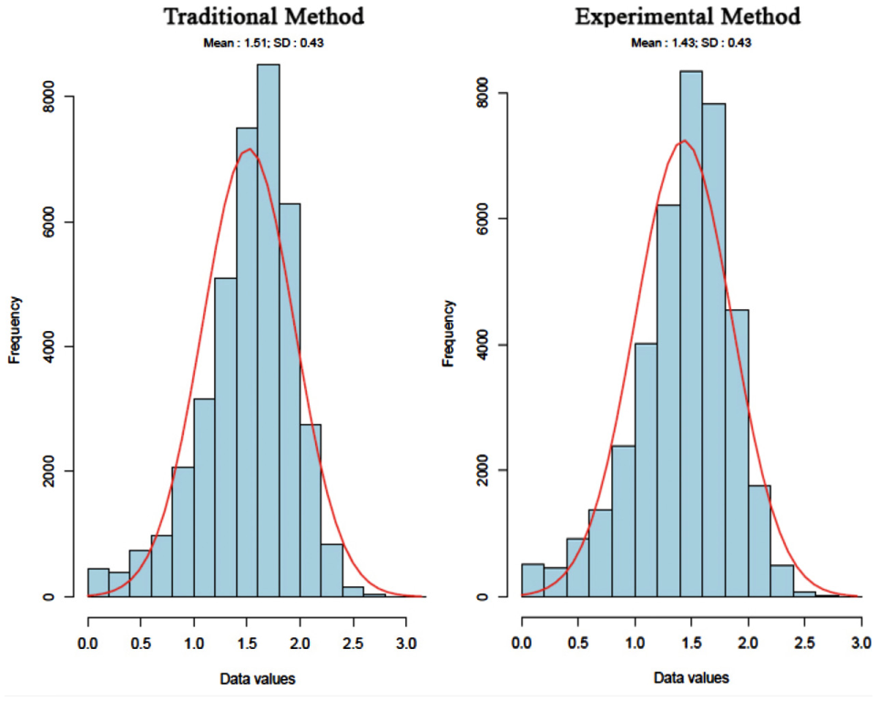
Stability distribution of users based on the WSI criterion.
Comparison
All algorithms were computed on the same computer with an Intel Core i5-5200U CPU 2.20GHz and 8Go RAM, using the free software R and the KMeansrcpp algorithm from the ClusterR package. Table 2 shows temporal averages of the different criteria, illustrating the interest of using the experimental week-to-week algorithm to cluster the transit users after a traditional simulation. Three other simulations are presented in this table: the experimental method with a one-year initialization to propose a fast clustering with an acceptable quality; the K-means++method to present the potential of K-means enhancements; and finally the experimental method with the K-means++results as initialization to show the complementarity between both enhancements.
Comparison of the Simulations
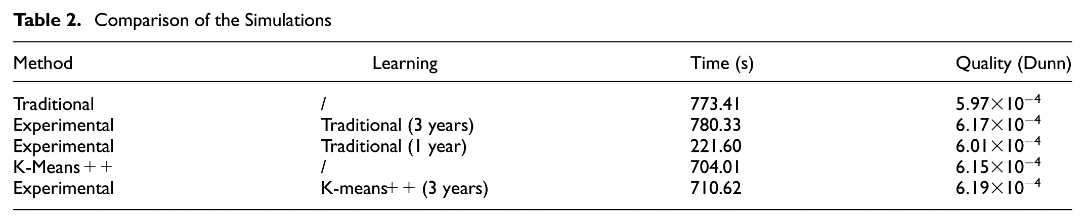
As expected, the week-to-week algorithm provides a very fast clustering of the 159 weeks (6.92 seconds) with a 3.2% higher quality clustering rate than the traditional algorithm. As its initialization consists in running the traditional method, however, the experimental one becomes slightly slower. A solution to make this experimental method faster is to reduce the initialization. This way, initializing with the first year of data, the algorithm takes 3.5 times less time and maintains a similar quality and stability to the traditional one.
By contrast, the presented method is compared with a usual K-means enhancement, the K-means++. Both simulations proposed a similar clustering quality, but the experimental method takes a longer computation time due to its initialization. The final simulation proposed seems to solve that issue. Indeed, running the week-to-week algorithm after the K-means++makes it possible to obtain the best quality results in a similar computation time.
Conclusion
This article proposed an analysis of transit users’ behaviors in Gatineau, Québec, involving a clustering of smart card data. Using the K-means algorithm, it presented a comparison of a traditional clustering method and an experimental week-to-week clustering algorithm leading to the demonstration of the evolution of users’ behavior. Assuming that clusters can evolve through time, traditional clustering techniques are not suited to follow such evolution. An emerging technique, based on inferring an optimized initialization in a week-to-week clustering through a distance-based K-means algorithm, shows evolution in cluster centers. This way, the algorithm clusters individual behavior vectors, created from counting the number of trips made by the users each day of the weeks of the study period. Nevertheless, this analysis leads to a common transit issue in this case—holidays are modifying users’ behavior and generating slightly skewed results. Assessing the behavior evolution, most of the cluster centers are stable and similar to the traditional method results, however, some follow seasonality, thus helping transit planners to gain a better idea of users’ behavior changes. Forecasting methods could now be applied on these cluster centers to estimate behavior changes in groups, and particularly for holiday week cases. Plus, the algorithm calculated an individual stability criterion on each transit user to help planners to understand users’ behavior instability level, a major criterion in the possible evolution of behaviors.
This emerging clustering methodology presents some limitations. Assessing the clustering quality enhancement, the experimental algorithm needs an initialization to start, consisting in running the traditional method on at least one year of data. Knowing that the computation time of the incremental clustering is around seven seconds for the three years of data, adding an initialization of at least 200 seconds will considerably increase the total computation time. This method thus needs a fast initialization with a good quality to show its entire potential against common K-means enhancements. Furthermore, the occurrence of holiday weeks is a common problem in transit planning. The methodology proposed a learning function so as not to be skewed by the previous holiday weeks. Based on the mean of the previous results, it helps the algorithm to converge to the best local optimum and allow planners to follow the evolution of the centers. To gain a more accurate model, this function should take external parameters, like network change or influence of weather, into consideration. The advantage of the experimental method is in allowing transit planners to follow the evolution of users’ behavior. It also outperforms the traditional method in computation time, clustering quality, and analysis level, but it is still insufficient to understand behavior changes entirely. Indeed, the algorithm was computed on simple behavior vectors to show its relevance. Working on the number of trips performed each day of the week might not bring enough details to get all the information about behavior changes. Dividing the days into four parts, thus creating a more detailed behavior vector with 28 components, could show an improvement. Finally, the method was applied solely with vectors from temporal-only data; a spatiotemporal combination should produce more interesting results.
Assessing the fact that clusters can evolve brings out the idea of splitting and merging clusters. This way, a radical change in users’ behavior could force them to converge into one cluster or, conversely, to be split into two different clusters. This evolution of the number of clusters could be found, particularly on holiday weeks.
Footnotes
Acknowledgements
This work was possible thanks to the collaboration of STO. Funding is provided by the Natural Sciences and Engineering Research Council of Canada (NSERC), Mitacs (grant # FR27498), the Société nationale des chemins de fer français (SNCF) and Keolis.
Author Contributions
The authors confirm contribution to the papers as follows: study conception and design: AV, MT, CM; data collection: MP; analysis and interpretation of results: AV, MT, CM; draft manuscript preparation: AV, MT, CM. All authors reviewed the results and approved the final version of the manuscript.
The Standing Committee on Urban Transportation Data and Information Systems (ABJ30) peer-reviewed this paper (19-00997).