
Abstract
In this paper, a combined model of auto-transit assignment is introduced based on two complementarity formulations in the literature. The model accounts for interactions between the auto and transit modes through non-separable asymmetric demand and cost functions. A path-based solution algorithm is presented based on the three ideas of decomposition, column generation, and linearization, which have proved to be effective in tackling large-size networks. Numerical results over the Chicago sketch network suggest that the algorithm converges quickly within the first iterations, but is less effective as the solution gets closer to the neighborhood of the equilibrium solution. The sluggish convergence behavior is attributed to the difficulty of searching the space of strategy-based transit assignment model.
Traffic assignment (TA) seeks to estimate the distribution of travel demand in a transportation network and the resulting link and path travel-times. Such information supports important urban planning functions such as evaluating and selecting infrastructure projects, and making policies related to travel demand management and control. Given its importance, TA models and their solution algorithms have been a recurrent theme in transportation research.
In urban travel forecasting, it is well known that TA is the fourth and the last step of the so-called four-step model, which also includes trip generation, trip distribution, and modal split ( 1 ). While the four-step model remains the state-of-the-practice in transportation planning, its shortcomings have been known and criticized for decades ( 2 , 3 ). A widely cited flaw is the inconsistency caused by the inability of a sequential procedure to capture the inherent interdependence between the steps. Consequently, many have attempted to integrate all or part of the four steps into various “combined” models ( 4 – 7 ). The state-of-the-art on these models has evolved to include various features to improve the realism of the model representation, such as user heterogeneity ( 4 ), composite mode choice ( 8 ), non-separable/asymmetric cost functions ( 5 , 7 ), and demand-side uncertainty ( 6 , 9 ). However, large-scale applications of these combined models are rare in the literature, mainly because the computational tools for transit assignment are relatively underdeveloped ( 4 , 5 ).
Mathematically, combined TA models can be formulated as one of the following: a nonlinear program, a variational inequality problem (VIP), a fixed point (FP) problem, and a nonlinear complementarity problem (NCP) ( 10 ). Of these approaches, nonlinear programming is probably the most widely used, but it is also more restrictive than the other approaches in that it requires symmetric cost functions ( 6 ). Therefore, most advanced models are formulated as VIP, FP, or NCP models, among which NCP models have been studied to a lesser extent (see [ 4 ] or [ 6 ] for examples).
Among combined TA models with two or more modes of transportation, namely “multi-modal” TA models, early studies often treated the transit mode as a dedicated service with a fixed cost between origin-destination (O-D) pairs. More sophisticated models have been proposed, however, to treat the transit mode through a “frequency-based” assignment ( 11 – 14 ). At the core of a frequency-based assignment model is the assumption that transit passengers use “strategy” to navigate through transit networks, which captures, with reasonable behavioral realism, how the passengers make choices at a transit stop where multiple lines are available.
The solution of the multi-modal TA problem has been mostly based on the diagonalization algorithm ( 15 ), the method of successive averages ( 16 ), and sensitivity-analysis based methods ( 17 ). Application of these methods on large-scale congested networks, to the best of the authors’ knowledge, has been rather limited, and hence their performance in real-world applications is largely unknown.
In recent studies, it has been recognized that the structure of the NCP model lends itself well to many efficient solution methods in large-scale problems. As a result, NCP assignment models of auto or transit mode have received more attention in various applications, for example, O-D demand estimation ( 18 ), network design problems ( 19 – 21 ), facility location problems ( 22 , 23 ), and congestion toll pricing ( 24 ). In spite of these efforts, however, there is still a gap in the literature on extending the NCP model to a multi-modal setting with a transit mode. This study aims to fill this gap by presenting a new NCP model which integrates TA and mode choice between auto and transit modes. Our study will leverage on the previous works by Aashtiani ( 25 ), which developed an NCP formulation for auto user equilibrium assignment, and by Babazadeh and Aashtiani ( 26 ), which developed an NCP formulation for frequency-based transit assignment in a congested network. This paper contributes to the literature in the following directions:
A joint NCP formulation of auto-transit assignment is introduced by integrating two previous formulations. The new formulation allows for non-separable asymmetric cost and demand functions.
Based on Aashtiani’s algorithm ( 25 ), a solution algorithm, capable of tackling large-size problems, is presented.
The performance measures of the solution algorithm are examined and reported in large-scale (although the convergence is not proven).
Complementarity Formulations for TA
A TA formulation is described here as “path-based” if it is written in relation to path-flow variables. Two separate path-based NCP models can be distinguished in the literature for auto and transit modes. These models are briefly introduced in next two sub-sections followed by a general description of their solution.
Path-Based Auto Assignment Model
The assignment of auto users is based on the concept of user equilibrium. In transportation literature, such equilibrium is often stated as Wardrop’s first principle which is “at equilibrium, for each O-D pair the travel-times on all the routes actually used are equal and less than the travel-times on non-used routes” ( 25 ). Under some mild assumptions, for example, links between volume and delay functions being continuous and non-decreasing, Aashtiani ( 25 ) proved that the user equilibrium problem with elastic demand functions can be stated as a path-based NCP model. Given that, Aashtiani’s model can be stated as:


where
R: set of trip origins.
S: set of trip destinations.
and
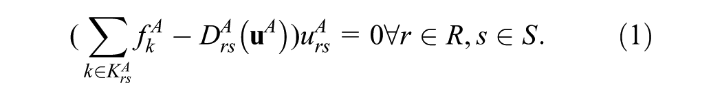
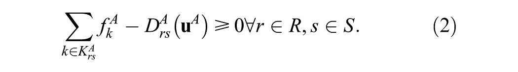
In the above model, Equations 1 to 3 state the flow conservation in a complementarity form and Equations 4 to 6 are those commonly used to describe Wardrop’s first principle in auto assignment ( 27 ).
Aashtiani ( 25 ) suggested that the volume-delay function of the above model can take a general form and need not depend only on its own traffic flow. As a result, more sophisticated volume-delay functions, as in two-way streets or intersections, may be incorporated into the model. He further extended the model for multiple modes of transportation while considering the demand as a function of all modes. This model has been recognized as the first model in the literature allowing for non-separable volume-delay and performance-demand functions ( 5 ). However, its representation of transit mode is still quite simplistic in the sense that it does not account for features like optimal strategies later developed in the literature.
Path-Based Transit Assignment Model
The behavior of transit users is more complex than that of auto users and is often modeled using the concept of “optimal strategy.” A “strategy,” first introduced by Spiess ( 11 ), is a set of rules that allows a transit user to navigate through a transit network ( 28 ). In most recent transit assignment models, it is assumed that transit users seek to minimize their “expected” travel-times through finding the optimal strategies ( 26 ).
The optimal strategy assignment with fixed travel-times was formulated by Spiess and Florian ( 12 ) as a linear programming problem in the space of link-flow variables. Later Babazadeh ( 14 ) proved that the optimal strategy assignment problem can be alternatively expressed in the space of path-flow variables. To formulate this problem, the following NCP model was proposed ( 26 ):


where
and
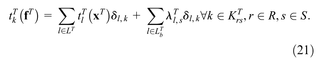
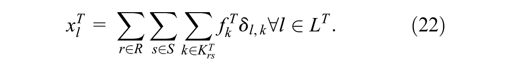
The first six equations of the above model are adopted from Aashtiani’s model. Equations 9 to 11, again, stand for the flow conservation. Babazadeh (
14
) also proved that, using auxiliary variables
A few remarks are in order here. Equations 9 to 20 may be regarded as an extension of the optimal strategy assignment proposed by Spiess and Florian (
12
) in a complementarity form. To the best of the authors’ knowledge, Babazadeh (
14
) and Babazadeh and Aashtiani (
26
), while accounting for congestion effects, are the only studies in the literature that report large-scale applications of asymmetric strategy-based transit assignment. Note that, similar to Aashtiani’s model, an elastic demand function, i.e.,
Solution of Complementarity Assignment Models
To solve the complementarity assignment model 1 to 6, an algorithm based on decomposition, column generation, and linearization was proposed by Aashtiani ( 25 ). A similar algorithm was later developed to the transit model by Babazadeh ( 14 ). According to the authors’ knowledge, no official proof has been reported for the convergence of the algorithm in a general case. However, the convergence has been supported by empirical studies on various examples in the literature ( 25 , 26 ). Aashitiani’s solution algorithm is briefly described below ( 25 ).
The complementarity assignment model typically has intractable numbers of solution variables and constraints. In the decomposition technique, this problem is broken into smaller sub-problems each corresponding to a single O-D pair. While solving each sub-problem, the variables corresponding to other O-D pairs are fixed. Accordingly, rather than solving the problem simultaneously for all O-D pairs, the algorithm iteratively solves the sub-problems and updates the resulting variables in the network.
Even with decomposition, enumerating all paths for a single O-D pair is still prohibitively expensive. To bypass a full enumeration of paths, the column generation technique is used, which only generates and keeps a small number of “working paths” as needed. Working paths for each O-D pair are those actually used by travelers and can typically be found by path-finding algorithms.
Finally, a Newton-type linearization technique is applied to tackle the non-linearity arising in the problem. Given that the complementarity assignment model has a general form as


the problem, in a given solution


The original Equations 24 to 26 are then solved by successive linearizations as Equations 27 to 29 and the current solution
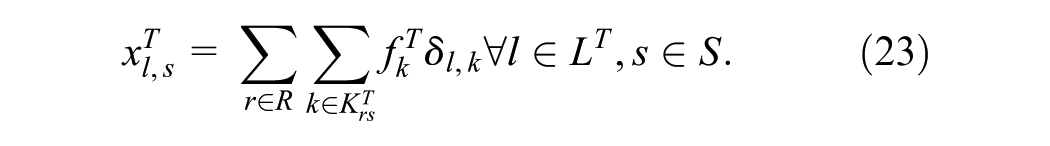
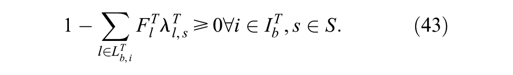
The Joint Formulation for Auto-Transit Assignment
The two previous path-based formulations can be integrated into a single NCP, in which demand and travel-time functions are expressed in relation to
The problem P (joint formulation)


where


Application of vectors of travel-times and flows, that is,
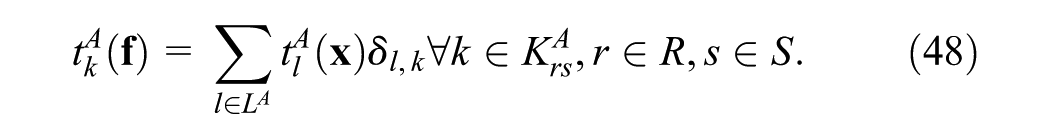
Auto equilibrium based on Wardrop’s first principle, through Equations 30 to 35 ( 25 ),
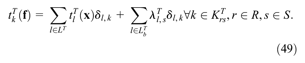
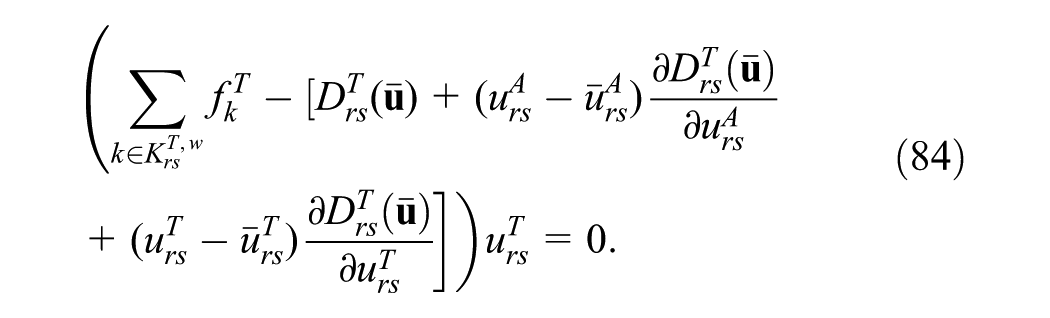
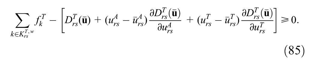
Transit equilibrium based on optimal strategy, through Equations 36 to 47 ( 26 ), and
Interaction/trade-off between the two modes in cost/demand functions, by considering
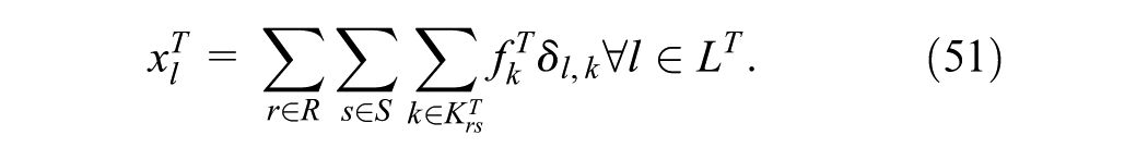
It is worth mentioning that, while only two modes are considered in the formulation, extending the model to include multiple auto and transit modes is straightforward.
Solution Method
The model of this paper is a complementarity problem with a similar structure to the previous models introduced earlier. Therefore, the same three techniques of decomposition, path generation (column generation), and linearization are adopted to solve this problem.
Decomposition
First the problem is decomposed into sub-problems corresponding to each O-D pair and each of them is solved iteratively. The sub-problem corresponding to (r,s), that is, the decomposed version of the problem P for a single O-D pair (r,s), can be written as follows:
The sub-problem SP(r,s), for r∈R, s∈S:


In the above single O-D formulation for (r,s), r∈R, s∈S, the new notations applied are
Furthermore,

While solving the sub-problem SP(r,s), the variables associated with the O-D pairs other than (r,s) are considered to be fixed. The obtained
Path Generation
In each iteration, path generation involves determining the single shortest path between O-D pairs for each mode. As the algorithm proceeds, new shortest paths generated for an O-D pair are introduced to the model. These paths, denominated as “working” or “active” paths, are stored for each O-D pair throughout the iterations of the algorithm.
Following the notations used by Babazadeh and Aashtiani ( 26 ), let us define:
In the path generation phase, the above notations are considered in SP(r,s) instead of
Linearization
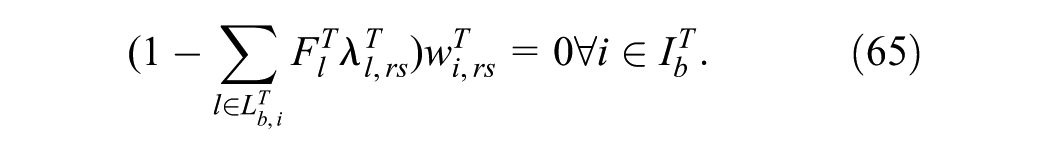
As mentioned earlier, the idea of linearization is to start with an initial feasible solution,
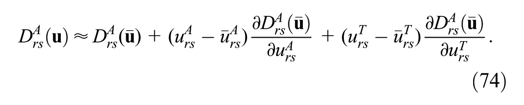
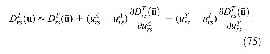

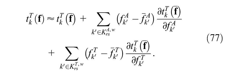
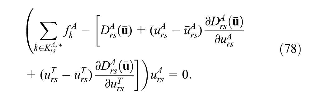
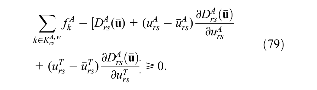
Details on how to calculate partial derivatives are omitted here for brevity. Based on the approximations in Equations 74 to 77, the linearized version of
The linearized sub-problem


To start the linearization process in solving the above problem, a good initial solution may be shortest paths. For the transit mode, the shortest path further depends on auxiliary variables
Termination Criteria
To check the convergence of the assignment algorithm, the well-known relative gap and a measure of demand error are applied. In the following, these measures are introduced.
Relative Gap
Relative gap is a common stopping criterion in the literature of TA algorithms ( 8 , 20 ). It is used to measure how far away the current solution is from the true equilibrium. For the auto mode, the relative gap can be defined as:

where


Based on the notations introduced earlier, the following definition of the relative gap can also be applied to the path-based transit assignment:

where


To integrate both auto and transit relative gaps into a single measure, the following relative gap is adopted in this paper:

where
Similar to Equation 104, but at the scale of a single O-D pair, another relative gap is used here in the linearization process where

where

Demand Error
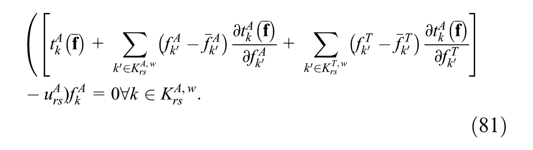
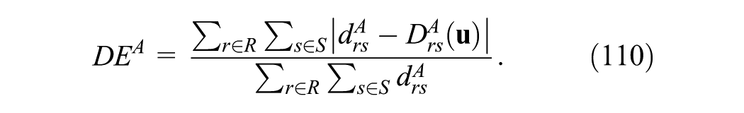
Another issue that may appear in multi-modal assignments is the amount of misplaced O-D flow for each mode ( 29 ). Following Aashtiani ( 25 ), this issue is addressed in this paper by using a “demand error” criterion that indicates how much the amount of flow for one mode is compatible with the performance-demand function of that mode. For auto and transit modes, the demand error is defined as Equations 110 and 111, respectively:

The two measures of demand error are integrated as:
Also, for each O-D pair (r,s), r∈R, s∈S:
Solution Precision
To specify the precision of the assignment solution, two values of


While solving the sub-problem


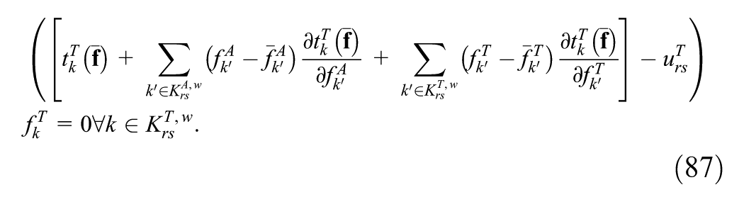
Solution Algorithm
Based on the main features of the solution, presented in previous sub-sections, Figure 1 provides a detailed description of the solution algorithm. The algorithm starts by generating an initial solution (i.e., single shortest paths) for both modes and initially setting the corresponding variables (lines 1–12). Prior to performing the main iterations including decomposition, path generation, and linearization, the algorithm checks whether or not the stopping criteria are already met (lines 13–16).
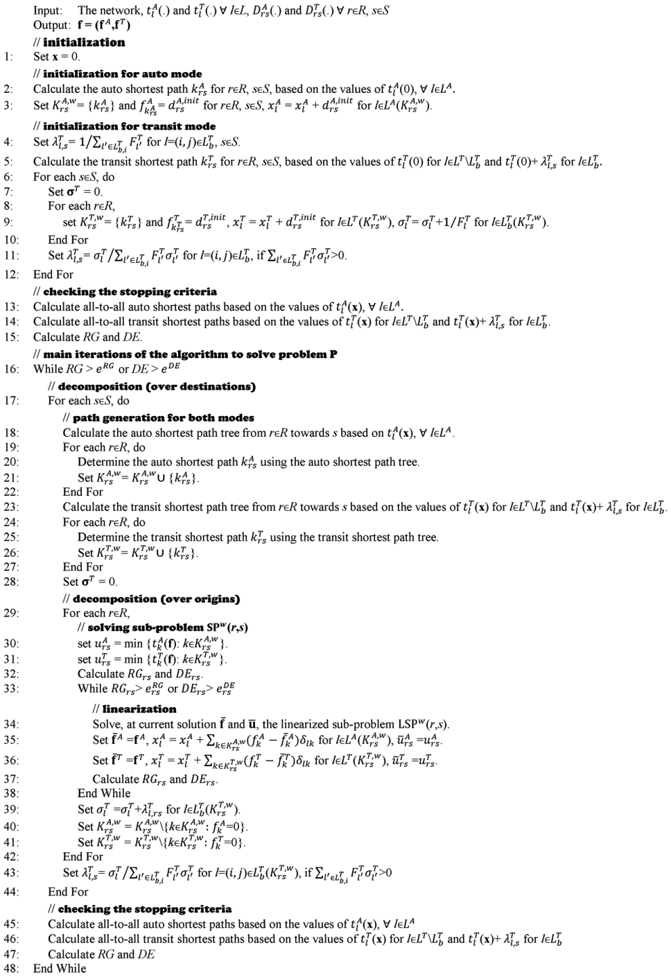
Solution algorithm for the auto-transit complementarity assignment model.
Within the main iterations of the algorithm (lines 16–44), the problem is decomposed into O-D pairs. The decomposition has two phases, one over destinations (line 17) and the other over origins (line 29). The selection of destinations or origins in the decomposition process may be done in a random way or any predefined order. As discussed earlier, new shortest paths need to be generated and introduced to the model when solving the decomposed sub-problems SP(r,s). But calculating a shortest path from a single origin to a single destination, in a worst case analysis, is computationally equal to calculating the shortest path tree. Since calculation of shortest paths can put a heavy computational burden on the algorithm, it is not performed separately for all O-D pairs. Instead, for both auto and transit modes, shortest path trees are generated at the same time from all origins to a single destination (lines 18–22 for auto and 23–27 for transit) and the sets of auto and transit working paths are updated (lines 21 and 26, respectively). This is carried out in this paper using the Dijkstra algorithm.
By decomposition of the problem into a single O-D pair for (r,s) with updated sets of working paths (already available from lines 21 and 26) and updated minimum travel-times (lines 30 and 31), the problem
After each single round of solving all decomposed sub-problems and updating the variables (lines 17–44), the two measures RG and DE are recalculated (lines 45–47). The algorithm proceeds through the iterations until the stopping criteria are ultimately satisfied (line 16).
Numerical Results
To explore the performance of the solution algorithm, the Chicago sketch transportation network is considered in this section. The Chicago sketch network is a rather large representation of the Chicago city transportation network, consisting of 387 trip zones, 933 nodes, 2950 links, and 93,513 O-D pairs with non-zero traveling demand. For illustrative purposes, 55 artificial transit lines are considered, each with a nominal frequency of 0.25 (vehicles/minutes), and it is assumed that auto and transit modes have a shared right-of-way throughout the network. Figure 2 shows the configuration of this network along with the transit lines. All details about transit lines and the Chicago sketch network (including link travel-times, capacities, and travel demands) may be found in Zarrinmehr et al. ( 20 ) and Bar-Gera ( 31 ).
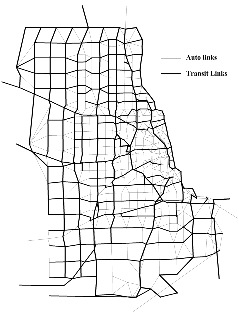
Topology of the Chicago sketch network and the transit lines ( 20 ).
The following implementation details and modeling assumptions are adopted in reporting the results in this section:
1) To capture various movements of transit users, a super-network is considered with a base layer corresponding to the auto mode ( 12 , 32 ). Transit movements are illustrated in relation to walking, boarding, alighting, and in-vehicle links, in a simple example in Figure 3 with transit lines L1 and L2 passing through stops 4, 5, 6 and 2, 5, 8 (denoted by 4(1)–5(1)–6(1) and 2(2)–5(2)–8(2)) respectively.
2) Given that: - - -
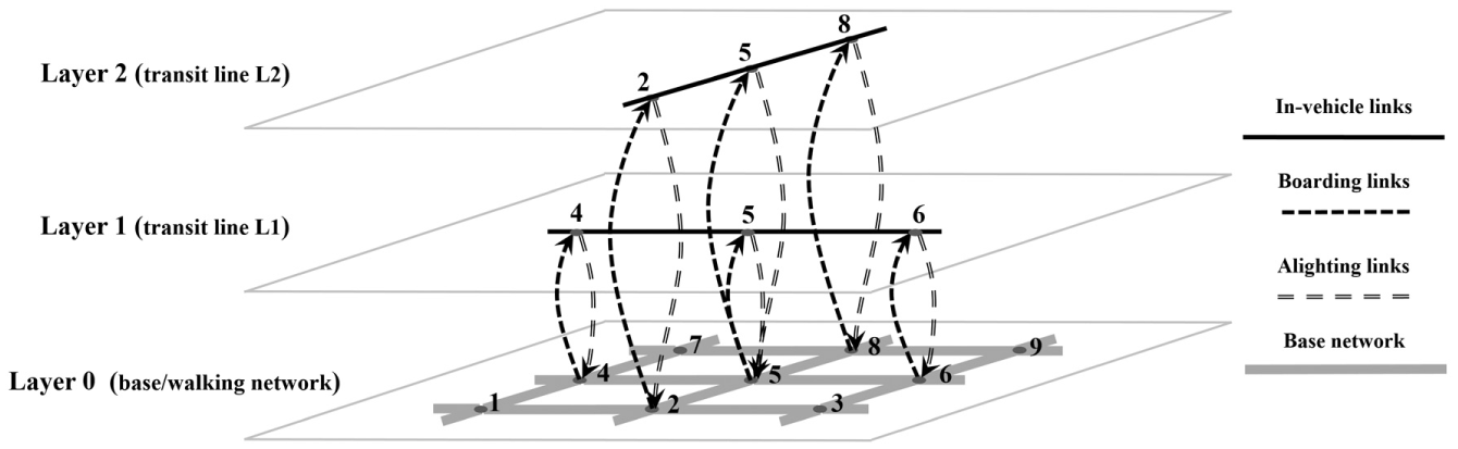
Example of super-network configuration.
an asymmetric auto travel-time, for the purposes of illustration, is adapted as follows:
3) For transit mode, the in-vehicle travel-time is considered to be 30% more than the auto travel-time on the same link, implying that the transit traffic stream moves slightly slower than the auto. Besides, there are boarding/alighting delays at transit stops, referred to as dwell-times. To formulate the dwell-time function, it is assumed that: - the in-vehicle link l∈ - τ is the period of time in minutes in which the travel demand values are expressed (i.e., demand values are expressed in relation to passengers per hour, then τ = 60 minutes), - - -

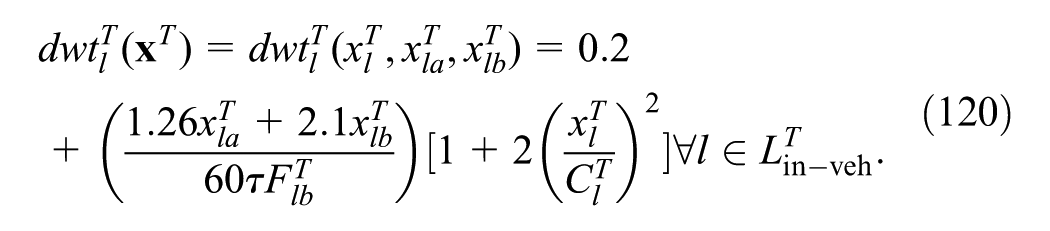
Based on the above definitions, the dwell-time is modeled empirically using the following asymmetric formulation ( 26 ):
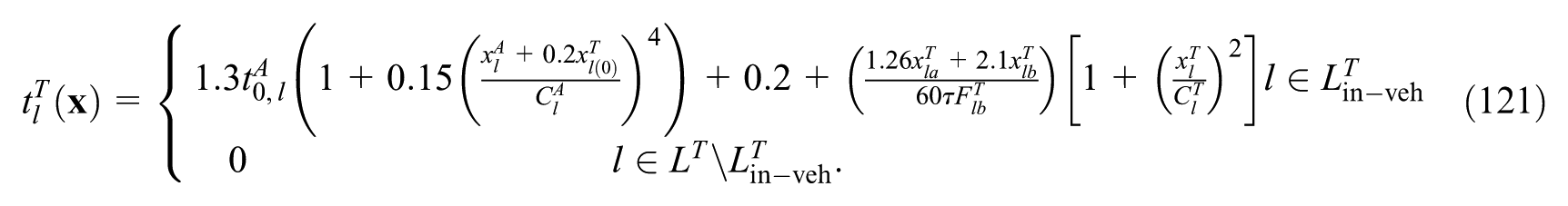
All in all, the travel-time function for a transit link can be stated as:
4) For an O-D pair (r,s), the total amount of travel demand,
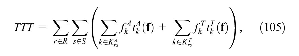
5) Walking is treated as a transit mode with infinite frequency at layer-0 (base network) of the super-network ( 12 ). The walking speed is considered to be 270 feet/minutes on average ( 33 ).
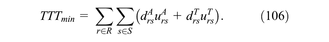
Based on the above assumptions, the algorithm was coded in Java programming language and executed on a server with an operating system of Red Hat Enterprise Linux Server release 5.4, a CPU of type Intel(R) Xeon(R) E5420 @ 2.50GHz, and 10 GB available RAM memory. The measures are reported during the successive iterations of the algorithm, which may offer a better insight about the performance of the algorithm. As a result, no pre-determined values are used for
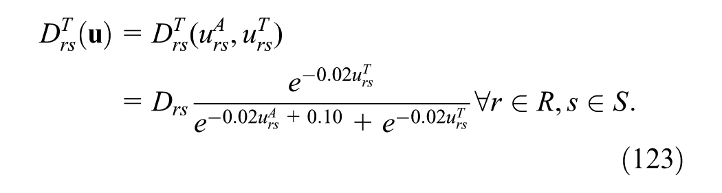
The results of running the program through 500 iterations are reported in Table 1. Note that calculations of performance measures are carried out only to monitor the performance of the algorithm. Therefore, the run-times associated with calculating these measures (i.e., lines 13–15 and 45–47) are not included in the last column in Table 1. The RG and DE measures, during the first 20 iterations of the algorithm (8.3 minutes of running the program), are also illustrated separately in Figure 4.
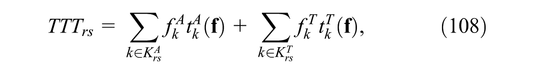
Performance Measures of the Solution Algorithm for the Chicago Sketch Network
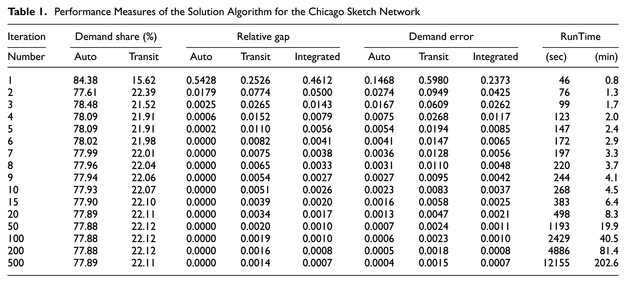
Performance measures for the Chicago sketch network: (a) relative gap and (b) demand error.
The results shown in Table 1 indicate that the auto relative gap converges quickly in the first few iterations of the algorithm. For the transit relative gap the convergence trend is also in line with the study of Babazadeh and Aashtiani ( 26 ) in the sense that the relative gap reduces sharply within the first iterations of the algorithm, but bears a low reduction, and then almost remains unchanged as the algorithm proceeds to further iterations. The table shows, for example, that the reduction of transit relative gap is only 0.0010–0.0007 = 0.0003, at the expense of 400 iterations beyond iteration 100 (i.e., iterations 101–500).
Similar to the relative gap measure, the values of demand error for both auto and transit modes in Table 1 suggest a rapid convergence within the first iterations, but remain almost unchanged beyond iteration 100. This observation can be justified, in part, with respect to the relative gap values of transit mode which are comparatively larger than those of auto mode. These gaps (errors), that is, the differences between the travel-times of existing transit paths and the minimum travel-times, are transmitted in both auto and transit demand errors through
Summing up, the results suggest that the algorithm converges effectively in the first iterations, but reveals a sluggish convergence behavior in a local region around the final equilibrium solution (e.g., beyond iteration 10).
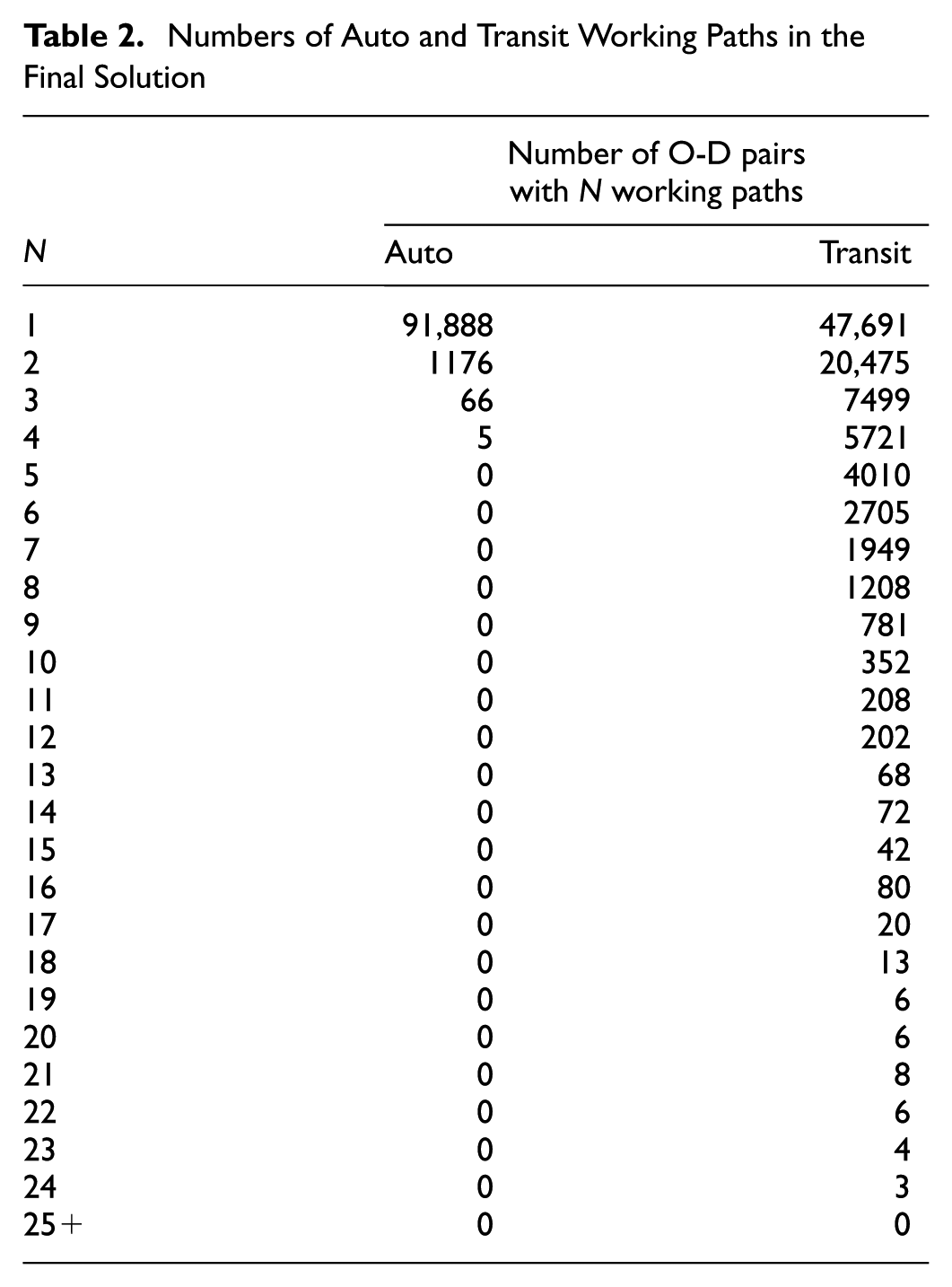
Finally, Table 2 presents the number of O-D pairs with N working paths for all values of N for both auto and transit modes. The results correspond to the solution obtained by performing 500 iterations of the algorithm. The total number of transit working paths, calculated from the results of Table 2, is 166,253. This number is by far (almost 76%) more than the number of auto working paths which is 94,458. The table also shows that there are no O-D pairs with more than four working paths for auto mode, whereas many O-D pairs have more than 10 working paths for transit mode. Such large numbers of working paths in the transit super-network explains why converging to highly precise solutions is more difficult for the transit mode than for the auto mode.
Numbers of Auto and Transit Working Paths in the Final Solution
Concluding Remarks
In this study, a joint NCP formulation, allowing for non-separable asymmetric cost/demand functions, was proposed for the combined auto-transit TA. The solution algorithm was built upon decomposition, path generation, and linearization, and performance measures were reported in relation to relative gaps and demand errors in the Chicago sketch network with 55 transit lines and more than 93,000 O-D pairs. Both measures were observed to converge rapidly in the first iterations of the algorithm, but remained relatively flat for the subsequent iterations. Also, in comparison with the relative gap, the demand error was found to be more resistant to convergence. After 100 iterations of the algorithm in the Chicago sketch network, the value of 0.0010 was obtained for both integrated relative gap and demand error.
Since not much work has been directed towards path-based multi-modal assignments, several directions may be identified for future research:
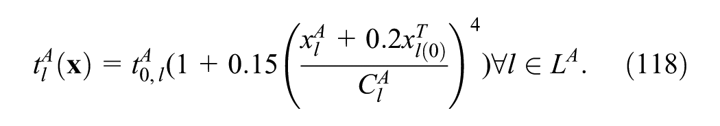
1- It was observed in both Babazadeh and Aashtiani (
26
) and this study that, as the algorithm proceeds to many iterations, the transit relative gap (and then the demand error in this study) would fail to achieve higher levels of accuracy (e.g., in the order of
2- Implementation of the solution algorithm may be extended to incorporate multiple auto/transit modes, or further modes other than auto and transit.
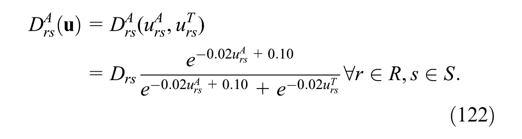
3- Pure auto and transit modes were considered in this study. Another research direction would be to extend the model to address composite modes of transportation, as well.
4- In many time-consuming decision making problems, application of paths information in assignment sub-models has been observed to notably speed up the solution algorithms ( 19 , 20 ). The proposed assignment tool, therefore, may be used as a sub-model to tackle advanced decision making problems such as multi-modal network design or pricing problems.
5- To report the results, several assumptions were made in this paper for illustrative purposes. The equilibrium and convergence behavior of the algorithm can be analyzed over these assumptions. For example, bus rapid transit systems (with exclusive transit lanes), various speed and frequency over transit lines, and different modal split functions may be considered in future research.
6- The performance of the solution algorithm may be compared with other multi-modal assignment algorithms in the literature, including those introduced to solve FP or VIP formulations. This comparison can be reported on speed, accuracy, or applicability as a sub-model in bi-level problems.
Footnotes
Acknowledgements
The authors are grateful to the three anonymous reviewers for their valuable insights and comments on this paper. The third author’s work was partially funded by U.S. National Science Foundation under the award number CMMI-1402911.
Author Contributions
The authors confirm contribution to the paper as follows: study conception and model development: HZA, HA; code implementation: AZ; analysis and interpretation of results: HZA, YMN, AZ; draft manuscript preparation: AZ, YMN, HZA; All authors reviewed the results and approved the final version of the manuscript.
The Standing Committee on Transportation Network Modeling (ADB30) peer-reviewed this paper (19-02434).