
Abstract
This research develops a system optimal dynamic traffic assignment (DTA) model for mixed traffic of human drivers and automated vehicles (AVs) and investigates network level mobility and energy impacts for different market shares of AVs. A methodology based on vehicle-specific-energy is proposed to estimate the energy consumption from the embedded spatial-queuing traffic flow model within the DTA formulation. Results with a test network indicate that potential travel time and energy consumption reductions are possible with increased AV market share in transportation networks. Results also report a decrease in travel time as high as 49% and energy consumption as high as 28% at the system level. The developed DTA model will be able to assist in transportation planning and the investment decision process by estimating the mobility and energy impacts in future transportation networks with mixed traffic of human drivers and AVs.
The trajectory of technological advancements suggests a transition of transportation networks to fully automated vehicles (AVs) in the future. Nevertheless, the exact timeline is uncertain as a result of several elements including progress in vehicle technologies development, public acceptance, AV policies and related legislation, and overall transportation infrastructure development and funding availability. For the immediate future, mixed traffic of automated and legacy human-controlled vehicles (HCVs) can be anticipated in transportation networks. Thus, it is high time to develop dynamic traffic assignment (DTA) tools for future transportation systems in which there is a significant share of AVs on the road. The primary goal is to assess the potential benefits for safety, mobility, and energy from long-term planning and short-term operational perspectives. AVs are expected to bring potential benefits to future transportation networks in relation to safety, mobility, energy, and productivity. In addition to significant safety impacts, the transportation networks are expected to receive boosts in mobility, congestion reduction, and throughput increase (1–5). Recent studies have confirmed that the market share of AVs will have a direct impact on the capacity of road networks (6, 7). Further, AVs can significantly cut down energy consumption for the transportation sector by following energy-optimal speed and acceleration profiles in different contexts including freeway merging and decentralized control (8, 9), traffic signal control ( 10 ), cooperative cruise control ( 1 ), and routing and operations (11, 12). Note that this research focuses on the operational benefits of AVs from a system perspective. It must be acknowledged that the overall impact may not always be favorable with increased accessibility, induced demand, and other undesired factors. That analysis is beyond the scope of this work. Several recent works, including (13–15), provide a detailed discussion of the cost–benefit of AV deployment in future, accounting for different transitional factors in both demand and supply sides of a transportation system.
Transportation networks with AVs are expected to experience a capacity increase during daily operations (1, 16). A close analogy is cooperative adaptive cruise control (CACC), under which capacity benefits are realized through flow smoothing and reduction in headways in the traffic ( 2 ). Existing literature includes many works relevant to the benefit analysis of CACC, mostly in a fine resolution using microsimulation (1, 17, 18). Except for a few, including (2, 3, 19, 20), the scope of most existing studies is limited to freeway sections and small arterials and they are not suitable for estimating network-wide impacts accounting for route and departure time choice behavior of the travelers. Studies (3, 20, 21) proposed a multiclass cell transmission model (CTM) and demonstrated the effects using custom DTA software with dynamic user equilibrium (DUE) behavior. Another work developed a system optimal DTA model focusing on dynamic lane reversal ( 22 ); however, the model does not account for mixed traffic of AVs and legacy HCVs. Recently, ( 23 ) developed a congestion-aware system optimal model using a link transmission model (LTM) for shared AVs that does not require the treatment for mixed traffic—multiclass DTA formulation. To fully understand the mobility and energy impact of AVs through system optimal DTA models, it is important to integrate mixed traffic behavior.
Moreover, none of the existing works have estimated the energy impacts at a network level from a system optimal DTA model. The challenges with energy estimation from first-order traffic flow models include: (a) individual vehicle speed estimation is not possible, (b) acceleration values can only be approximated, and (c) the energy estimate equations such as vehicle specific power (VSP) ( 24 ) show a high degree of nonlinearity causing the mathematical program-based DTA model to be challenging to solve.
This research aims to fill the gap in the literature in several ways. The goals are as follows:
To develop a mathematical program-based system optimal DTA model accounting for mixed traffic flows of AVs and legacy vehicles
To develop a first-order energy estimate methodology at the network level
To assess the mobility and energy impacts of the AV market share in a transportation network
This research develops a mathematical program-based DTA model. For a detailed discussion of different variants of DTA models, readers are encouraged to look at (25, 26). Further, ( 27 ) provides a comprehensive review of the DTA models with energy and environmental considerations. The rest of the paper is organized as follows: the next section discusses the impact of AVs on network capacity as a function of space headway; then, the system optimal DTA model for a mixed flow of AVs and HCVs is described; afterward, the methodology to estimate energy consumption from the spatial-queuing model, namely the CTM, is explained; next, the results from a test network are reported; and finally, the merits and limitations of the work are discussed, with directions for future extension.
Estimating Impact on Capacity for Mixed Traffic Flow
Modeling Heterogenous Traffic
Modeling mixed traffic flow has been approached in several past studies. From a macroscopic modeling perspective, the central idea is to represent traffic density in a weighted summation from multiple vehicle classes (28–30). The derivation follows the safe-following distance principle as described in (31, 32) and used in the works by ( 16 ) and ( 3 ). An effective headway expression similar to that in ( 21 ) was derived and then applied to the proposed system optimal DTA model through the flow propagation constraints. The concept of using headway—the gap between AV and legacy vehicles—is not new. However, the current study contributes uniquely in the following ways: (a) a safety-distance attribute for mixed flow is integrated into a mathematical program-based model which can be solved for traffic assignment—in contrast, Chen et al. ( 28 ) and Ghiasi et al. ( 30 ) mostly focused on the model to estimate capacity for a mixed flow and to analyze the sensitivity of capacity with different distribution and corresponding parameters; (b) a system optimal DTA model is developed, applying the concept through simulation-based CTM architecture; and (c) a method to estimate energy is developed from a mathematical program-based CTM and the energy benefits demonstrated at a system level.
Effect of Perception–Reaction Time
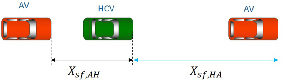
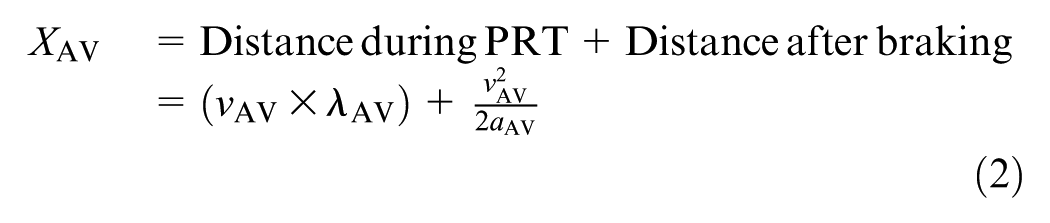
Consider a mixed traffic environment with automated vehicles (AVs) and HCVs sharing the same road. Figure 1 shows a situation in which an AV (red) is following an HCV (green), and an HCV is following an AV (red). The AV, in this case, does not need any human intervention while operating—that is, the automation level is 5 or higher. Among many distinct features of an AV, smaller perception–reaction time (PRT) compared with a human operator is expected. PRT involves four major driver tasks: detection, identification, decision, and response (33, 34). PRT values vary across drivers and types of road situations. The American Association of State Highway and Transportation Officials (AASHTO) mandates the use of 2.5 s for design and computational purposes. However, field data suggest that 90% of the drivers have PRT equal to or smaller than 2.5 s. For signal-timing purposes, the Institute of Transportation Engineers (ITE) recommends a PRT value of 1.0 s. Recent works suggest the PRT for AVs can be smaller than 0.1 s in general traffic conditions (16, 19, 35). Now, the safe-following distance—the space between consecutive vehicles to avoid a collision—is directly bounded by the PRT values. Accordingly, the density, speed, and flow of a traffic stream(s) will be affected.
Effect of PRT on safe-following distance for HCV and AVs.
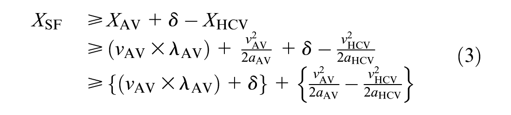
From kinematics, the safe-following distance between any two vehicles on a road segment can be computed. More details on safe-distance car-following behavior modeling can be found in (31, 32, 36). Consider an AV (red) following an HCV (green) as in the left part of Figure 1. Assume the traveling speed and maximum deceleration for the AV and the HCV are

With a PRT value of
Assume the distance between two vehicles at jam density—when the vehicles are at bumper to bumper—is
Approximating the Effect in a Spatial-Queuing Model
Stream of Multi-Class Flows
The previous section derives the impact of a smaller PRT value of an AV as a microscopic effect by which the behavior of each vehicle is modeled separately. To estimate the effect in an aggregate manner—when the interest is in the properties of a traffic stream in contrast to a single vehicle—macroscopic traffic flow models are more appropriate. One well-acknowledged avenue is the class of hydrodynamic theory-based traffic flow models ( 37 ), which can represent properties of a traffic stream in a reasonably accurate manner. Primary properties of interest include flow, density, shockwave propagation, and space–mean speed defined within a time–space boundary. Time–space diagrams of vehicular movement are at the core of estimating traffic flow properties.
Figure 2 shows a time–space diagram with the trajectories of four vehicles on a road (y-axis) for a short period (x-axis). The vertical line at the time
where

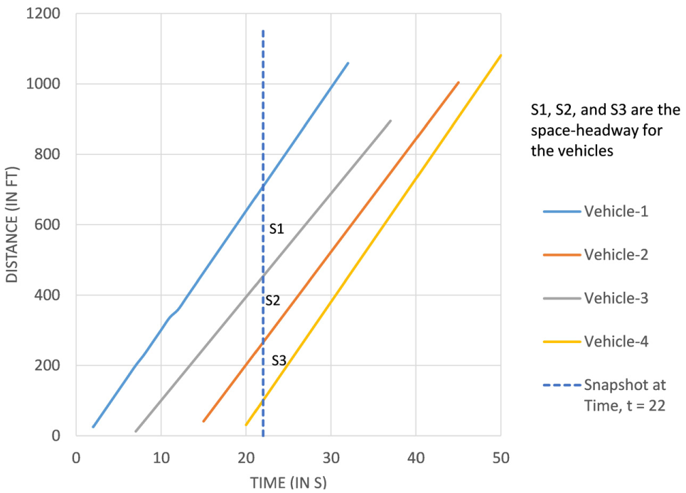
Space–density relationship within a time–space boundary.
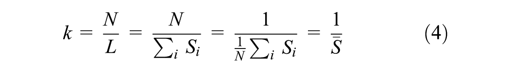
For a defined time–space region with vehicles keeping safe-following distance based on space headway and vehicle length

where
Θ is the total distance including vehicle length and the space between two vehicles at jam density.
Effects in a Mixed Traffic Flow of AVs and Legacy Vehicles
Consider a traffic stream with heterogeneous flow containing

where q = flow resulting from multiple vehicle classes.
From (6), the average spacing for any class
Now, denote
Note that, this is different from jam density
The backward wave propagation speed
System Optimal DTA Model for Mixed Traffic of AV and HCV
The system optimal DTA is formulated as a mathematical program in which the CTM acts as an embedded traffic flow model. The previous sections derived the expressions for density
Assumptions for the System Optimal DTA Model
The following assumptions are in place: (i) the formulation accommodates all the underlying assumptions of the CTM ( 40 ) and its linear relaxation ( 44 ); (ii) the class-specific density and speed values follow the hydrodynamic theory of traffic flow—this topic has not explicitly been discussed in this paper, mostly because existing works have already proven the consistency (19–21); (iii) vehicles travel at identical speed and the mobility and energy impacts are based on space–mean speed of the flow only; (iv) the solution from DTA reports a continuous flow solution and may not be realized in a real-world scenario; and (v) to estimate energy, boundaries have been defined for acceleration values to capture realistic propagation of flow, which is explained in a later section.
Notations, Symbols, and Path Notation
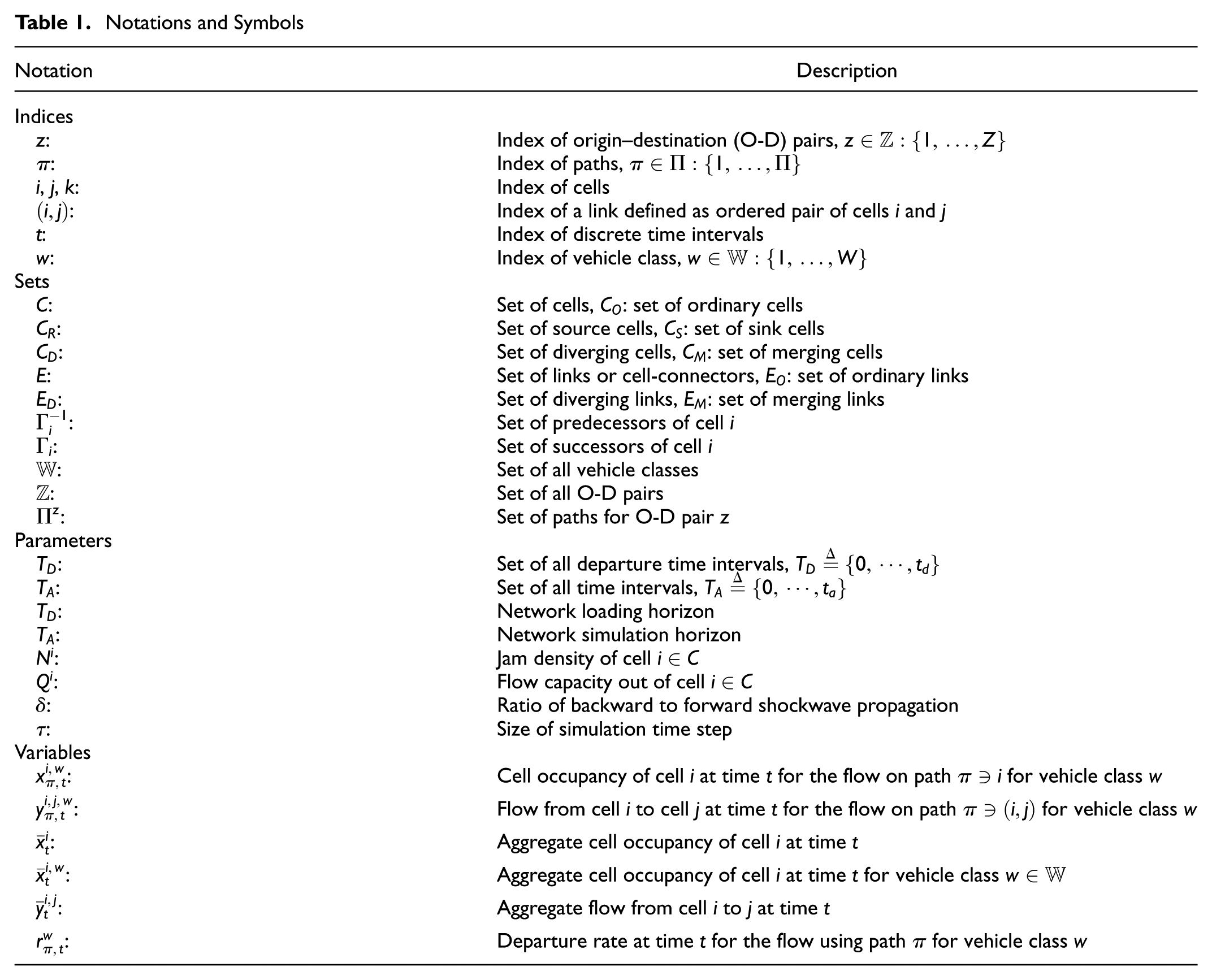
Notations and symbols are shown in Table 1.
Notations and Symbols
Note that each path
Initialization
CTM is initialized with zero flow and zero occupancies for the cells in the network for all vehicle classes:


Demand Satisfaction
The trip demand is specified for each O-D pair


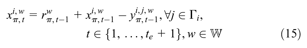
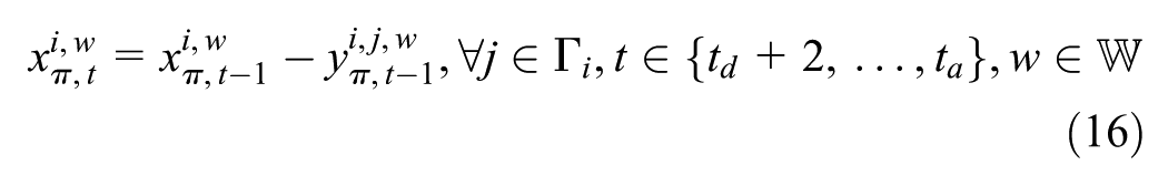
Occupancy Update
Source Cells (
)
During network loading period
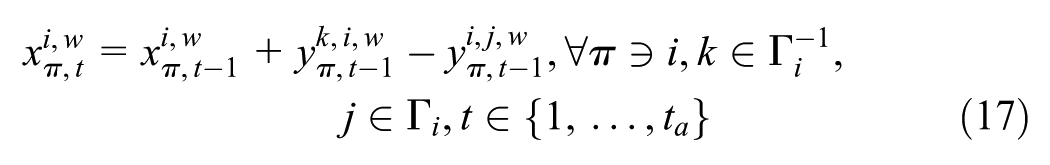
Ordinary Cells (
)
The ordinary cells
Diverging-Merging Cells (
)
For a diverging and merging cell,
Sink Cells (
)
A sink cell
Flow Propagation for a Mixed Flow of AV and HCV
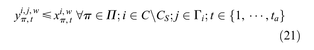
The proposed model uses the standard flow constraints similar to the linearized DTA formulation by Ziliaskopoulos ( 44 ) in which propagation rules are linearly relaxed to avoid nonlinearity in the mathematical program. It is acknowledged that this may cause the so-called “holding back” problem ( 48 ). Nevertheless, it is possible to use additional constraints and modified objective functions that aim to maximize the flow to reduce the holding back realizations in the network. Existing works ( 45 , 49–52) have used this linearization for traffic assignment problems with acceptable and reliable results.
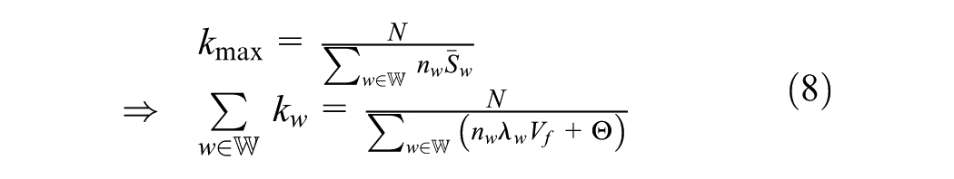
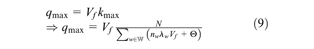
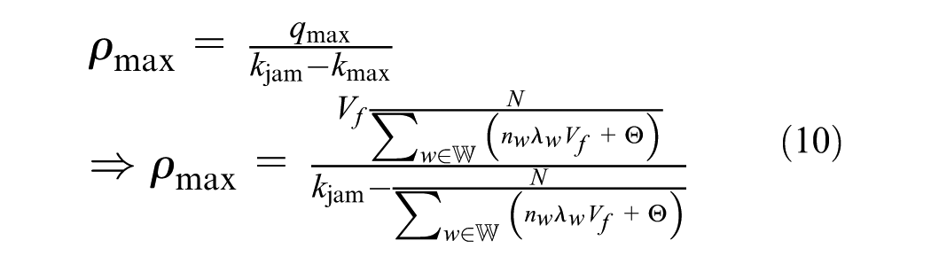
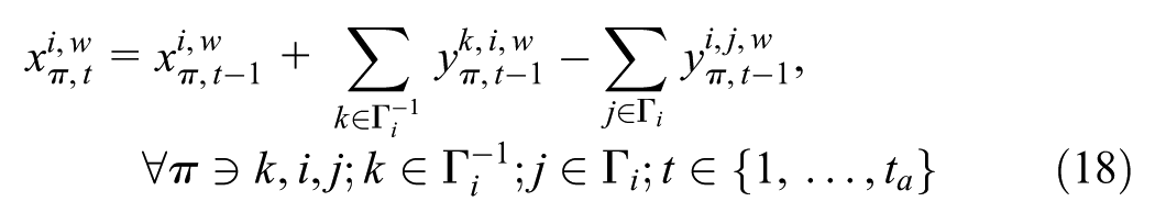
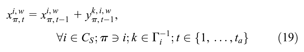
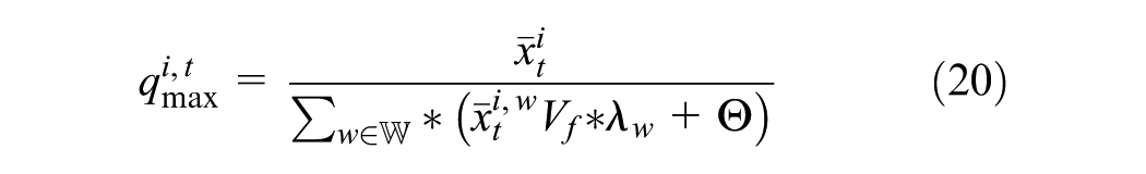
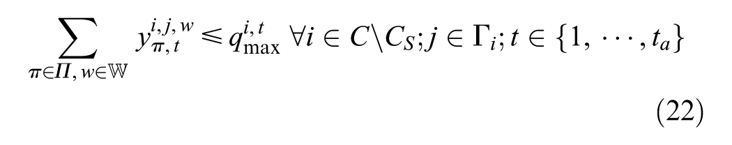
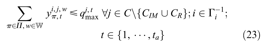
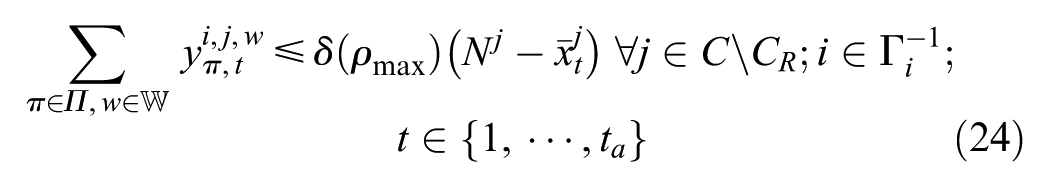
As has been shown in (8), at any point of time the maximum density possible is a function of the proportion of vehicles—AV and HCV—within a cell. Further, (9) defines the maximum flow from any cell
Further, the ratio
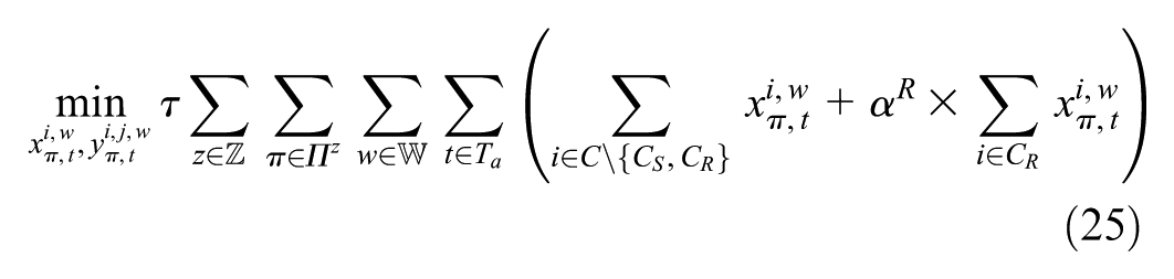
Objective Function
For a system optimal DTA, the total system travel minimization goal was applied. To account for “holding backs” in the source cells, the objective function has an explicit weight,
Solution Technique
Solver Specifications
The DTA formulation described above has nonlinear constraints and is nonconvex in nature. Although the flow constraints have been linearized and the objective function is linear, the proportional flow propagation 20 of multiclass vehicle flow makes the problem challenging to solve. The Artelys Knitro 11.0.0 optimization tool has been used to solve the DTA problem. Knitro options used: (I)
First-in-First-out Issues
It is acknowledged that the general math program-based DTA models for multiple O-D suffer from first-in-first-out (FIFO) violation (44, 47). Compared with a DUE model, the results from the developed system optimal formulation are expected to be less sensitive to FIFO violation, mostly because the equilibrium cost does not have a major role. Similar formulations have been used in recent studies (53, 54). Further, the developed formulation is a path-based formulation compared with the original LP-formulation by Ziliaskopoulos ( 44 ). Existing literature mentions several ways to account for FIFO with respect to the CTM. Carey et al. proposed to accommodate FIFO at different levels of resolution—cell, link, and route ( 55 ). This study has not scoped handing FIFO as a major goal for this paper because the order of impacts—mobility and energy—is not expected to be affected significantly from a lower degree of FIFO violation. The results presented in this paper are from a single destination case and this minimizes the impact. For a detailed discussion, please refer to (55, 56).
Energy Estimate from CTM
This section provides the methodology for estimating the energy from the average space–mean speed at cell level from the CTM. A VSP-based equation was followed to estimate the operating power requirements of an on-road vehicle. VSP estimates the instantaneous power per unit mass of the vehicle as a function of different factors including instantaneous speed, acceleration, aerodynamics, grade, and physics-based factors ( 24 , 57–60). The estimates using a VSP-based approach are consistent with fundamental kinematics and with emissions and fuel consumptions measures from sensors in real-world scenarios. Moreover, VSP equations can be customized for vehicle classes: light duty, heavy duty, hybrid, plug-in hybrid electric vehicle, and so on.
Vehicle Specific Power
VSP is expressed as ( 24 ):
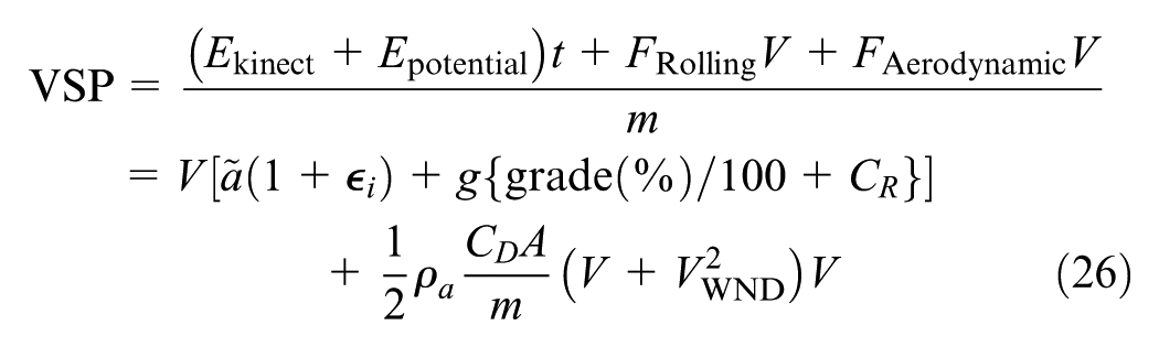
where
Light-Duty Vehicle (LDV)
Any passenger car and trucks with gross vehicle weight ratings (GVWR) less than 8,500 lb are designated as light-duty vehicles (LDV). Trucks are further classified into light light-duty trucks (LLDT) with weight ≤ 6,000 lb, and heavy light-duty trucks (HLDT) with weight > 6,000 lb. With standard parameters and coefficient in (26), the VSP for an LDV is computed as:
Heavy-Duty Vehicle (HDV)
Vehicles with weight greater than 8,500 lb are classified as heavy-duty vehicles (HDV). For an HDV compared with an LDV, the VSP equation is different because of the changes in a range of running weights, VSP binning, and engine standards. After adjustment, the scaled tractive power (STP) is computed as:
The grade ( %) is defined as the relative rise (or fall) of the facility in the longitudinal direction as a percentage of section length. A 5% grade of 1,000 ft means a vertical rise of 1,000 * (5/100) = 50 ft. Now, it is necessary to quantify the space–mean speed and an approximation of the cell-level acceleration from CTM.
Estimating Space–Mean Speed
The space–mean speed is considered for three different states:
Free-flow state
Queue-forming state
Queue-dissipation state
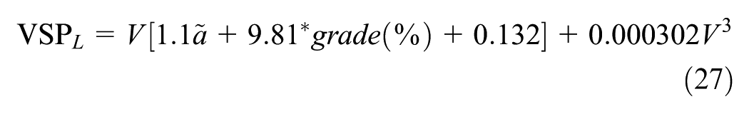
The space–mean speed depends on the density of the cell, and the available space inside a cell depends on the traffic states mentioned above. The fundamental flow–density relationship provides the space–mean speed of a cell at a specific time step. It is assumed that the vehicles, that is, the traffic flow, only travel from the boundary of the cells and the speed values are computed only at a time step, and not within time steps. For a time discretization of
Generalized merging–diverging cell configuration to demonstrate the space–mean speed and acceleration computation from CTM.
To compute space–mean speed for cell
Determine the inflow to cell

where
Determine the number of queued vehicles for cell

where
Find the density of the cell. For a congested state—either queue forming or queue dissipating—a certain portion of the cell may have already been occupied and it is possible to assume jam density for the queued vehicles with zero speed. Now, the effective density for the inflow is established. With

where

Find the flow rate: The flow rate,

Find the speed using the fundamental relationship:

Now, for a non-congested condition, there is no queuing of vehicles. Thus:

This is consistent with the CTM discretization condition:

where
Again, for a congested state with
Estimating Acceleration
A major challenge for estimating energy from macroscopic traffic flow models is the estimation of acceleration of the flow. Unlike the fundamental relationship among space–mean speed, density, and flow, estimating acceleration values is not straightforward. Studies suggest that the design acceleration values are different from those observed from field studies (61–63). Further, most passenger cars can only use a portion of the maximum acceleration and deceleration rate possible ( 61 ). This research uses the guidelines provided by the Traffic Engineering Handbook ( 64 ) for typical maximum acceleration rates that reflects linearly decreasing acceleration with increasing speeds.
Similar to space–mean speed, mean acceleration values can be estimated using basic kinematics. For any cell

Now, a known issue with first-order spatial-queuing models is that the acceleration and deceleration values can be unrealistically high when the time steps and the cell discretization values are not bounded, accounting for the acceleration. Consider two cases: (a) vehicles are entering a congested cell and joining a queue where the flow will decelerate from free-flow
Acceleration from Zero to Free-Flow
Using the Newtonian kinematics, distance traveled by a unit of flow is:

Now, the cell length,
Deceleration from Free-Flow to Zero Speed
Similar to the above case, for an effective deceleration rate

Now, the proper time step should be:

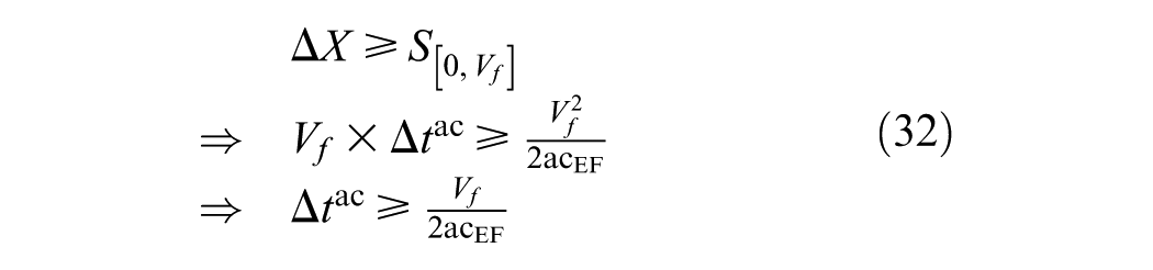
For a congested condition, the acceleration values will be defined by the reduced space–mean speed values and resulting densities. To avoid inconsistencies, it is also enforced that the resulting acceleration and deceleration values will be the minimum of the computed values from (30) and the bounds
Validation of Energy Estimate
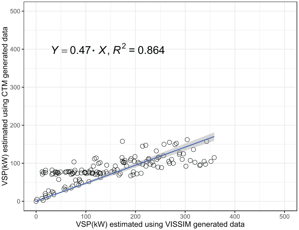
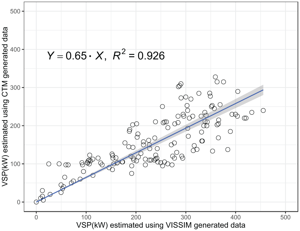
To validate the energy estimation approach, a freeway section was simulated both in the PTV VISSIM microsimulator and in CTM. Now, energy consumption is quantified using the VSP equation (27) for the entire link, from both CTM generated speed data as in (29) and VISSIM generated speed profiles for vehicles (aggregated for the freeway section). Figures 4 to 6 show the correlation between the estimates, and this study argues that for a first-order estimate this is reasonably accurate, with a Pearson’s
Correlation plot for VSP estimate from VISSIM and CTM under saturated condition.
Correlation plot for VSP estimate from VISSIM and CTM under partially saturated condition.
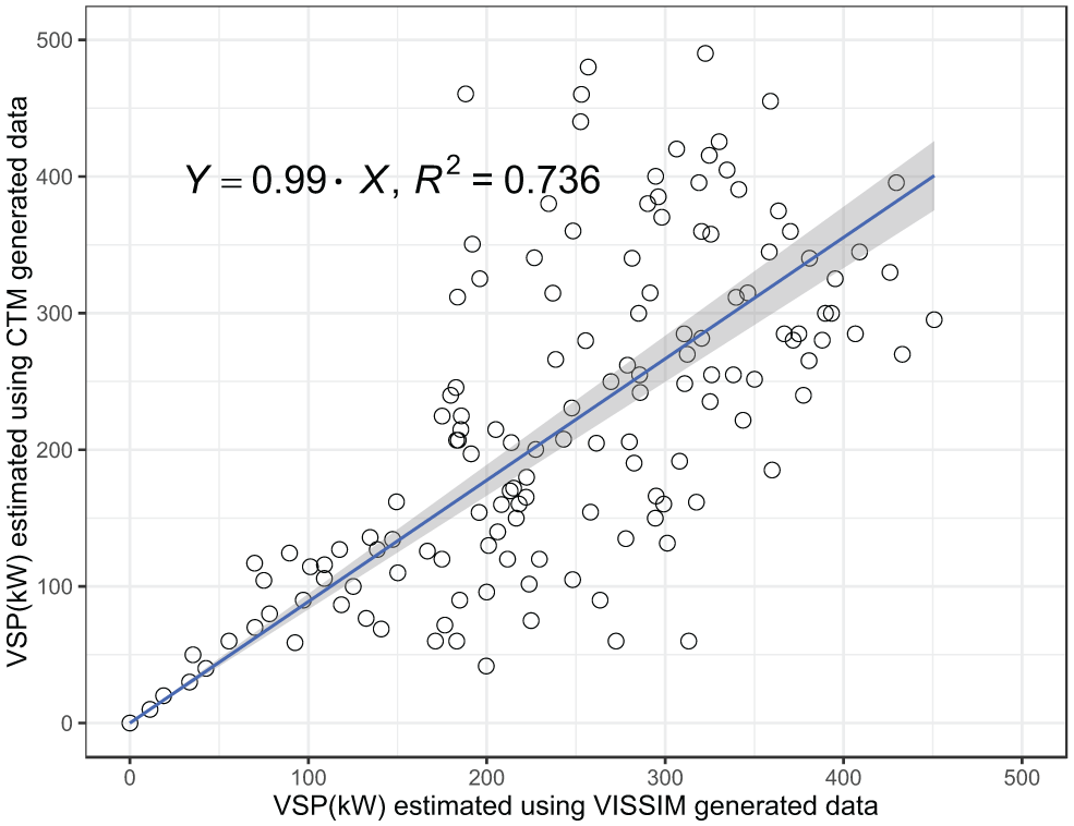
Correlation plot for VSP estimate from VISSIM and CTM under over saturated condition.
Numerical Results
The system optimal formulation for mixed traffic is implemented in a small test network with design parameters. The network is small; nevertheless, it has the representative attributes of the study’s core interests including:
Merging and diverging sections, and signalized intersections (with fixed signal settings)
Multiple O-Ds
Multiple paths for the investigation of flow redistribution
Figure 7 shows the graphical representation of the network (left), details on the CTM parameters (bottom left), and a sample cell representation of a signalized intersection (red node in the graph). Paths for each O-D pair are drawn in a different color. For instance, O-D pair
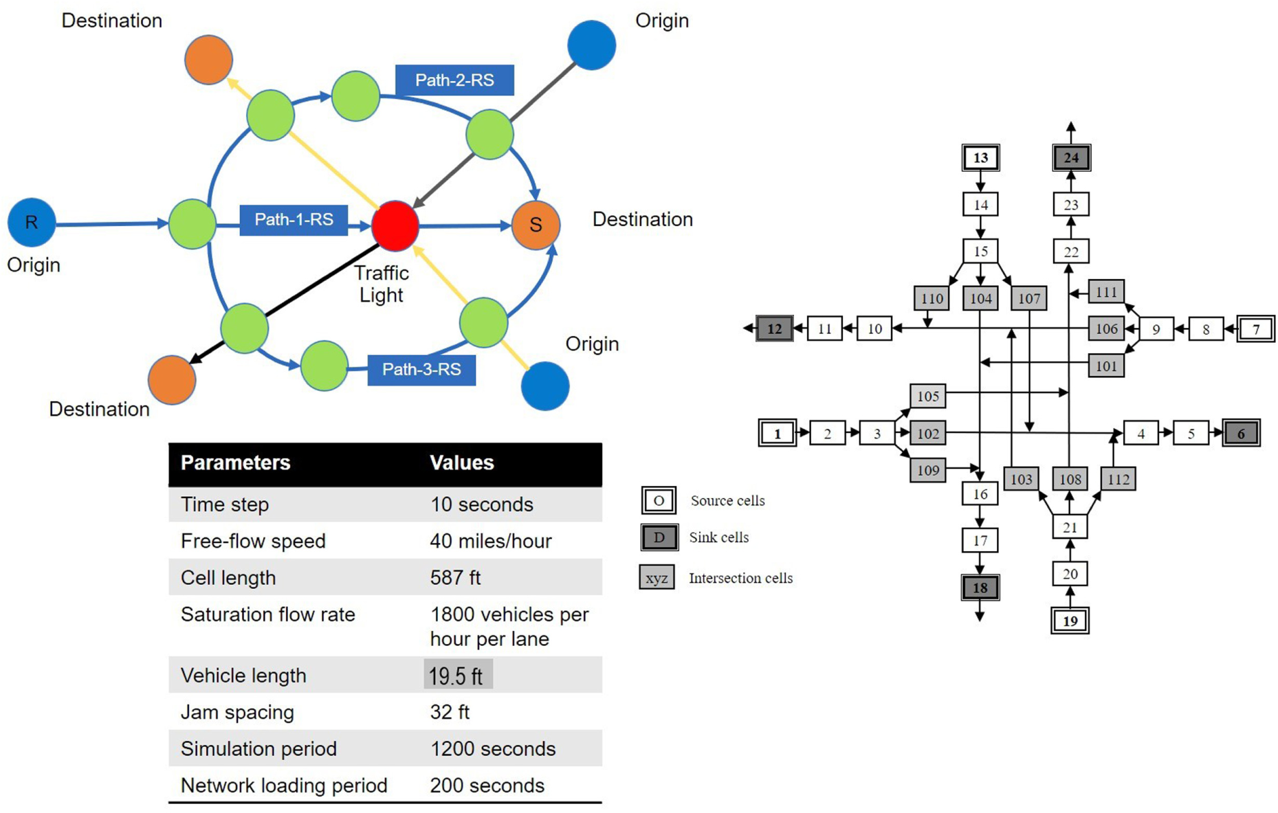
Test network details for which circles represent nodes in the network. Color codes: blue (origin), orange (destination), red (traffic light), and green (general nodes).
Vehicle Classes
The experimental settings consider two vehicle classes: AVs and HCVs. The HCVs are assumed to have a PRT value of 2.0 s and AVs can have PRT values ranging from 0.1 to 1.0 s. Each O-D pair has traffic demand that comprises both vehicle classes.
Effect of PRT Values on Travel Time and Energy
As discussed previously, smaller PRT values for AVs will increase the capacity at the system level and may reduce the energy consumption from the network. Given all network settings staying the same, the study examined the changes in total system travel time and energy consumption for different PRT values ranging from 0.1 to 1.0 s. Figure 8 shows the percentage change in system travel time compared with the base case with all HCVs (PRT = 2.0 s). The results confirm that smaller PRT values will lead to a decrease in system travel time. In addition, it can be seen that the gain in travel time reduction is smaller when the PRT gets smaller than 0.65 s.
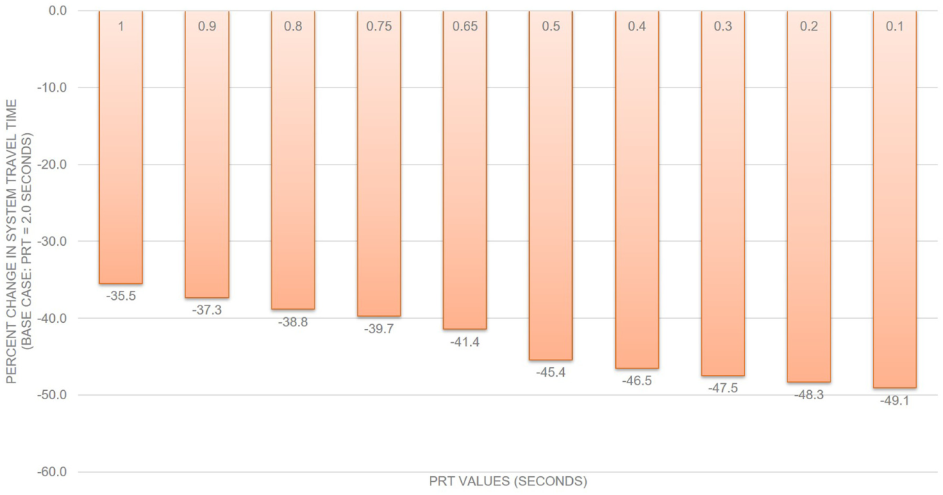
Change in total system travel time with different PRT values.
Figure 9 exhibits the percentage changes in energy consumption for different PRT values. The trend is similar to that found for the system travel time. However, the maximal energy gain (28.7%) is smaller compared with that of system travel time (49.1%).
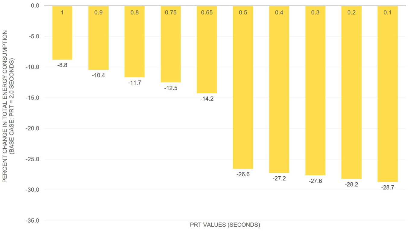
Change in energy consumption with different PRT values.
Impact of AV Market Share
Next, the impact of AV market share on the system travel time and energy consumption is investigated. For a fixed O-D trip demand, the market share of AVs in the network is gradually increased to explore the effects at the system level. The PRT value of AVs is realized at 0.65 s. Figures 10 and 11 show the system travel time and energy consumption changes, respectively. After a sharp gain starting at 20% AV share, the reduction in system travel time and energy consumption become smaller, but not negligible.
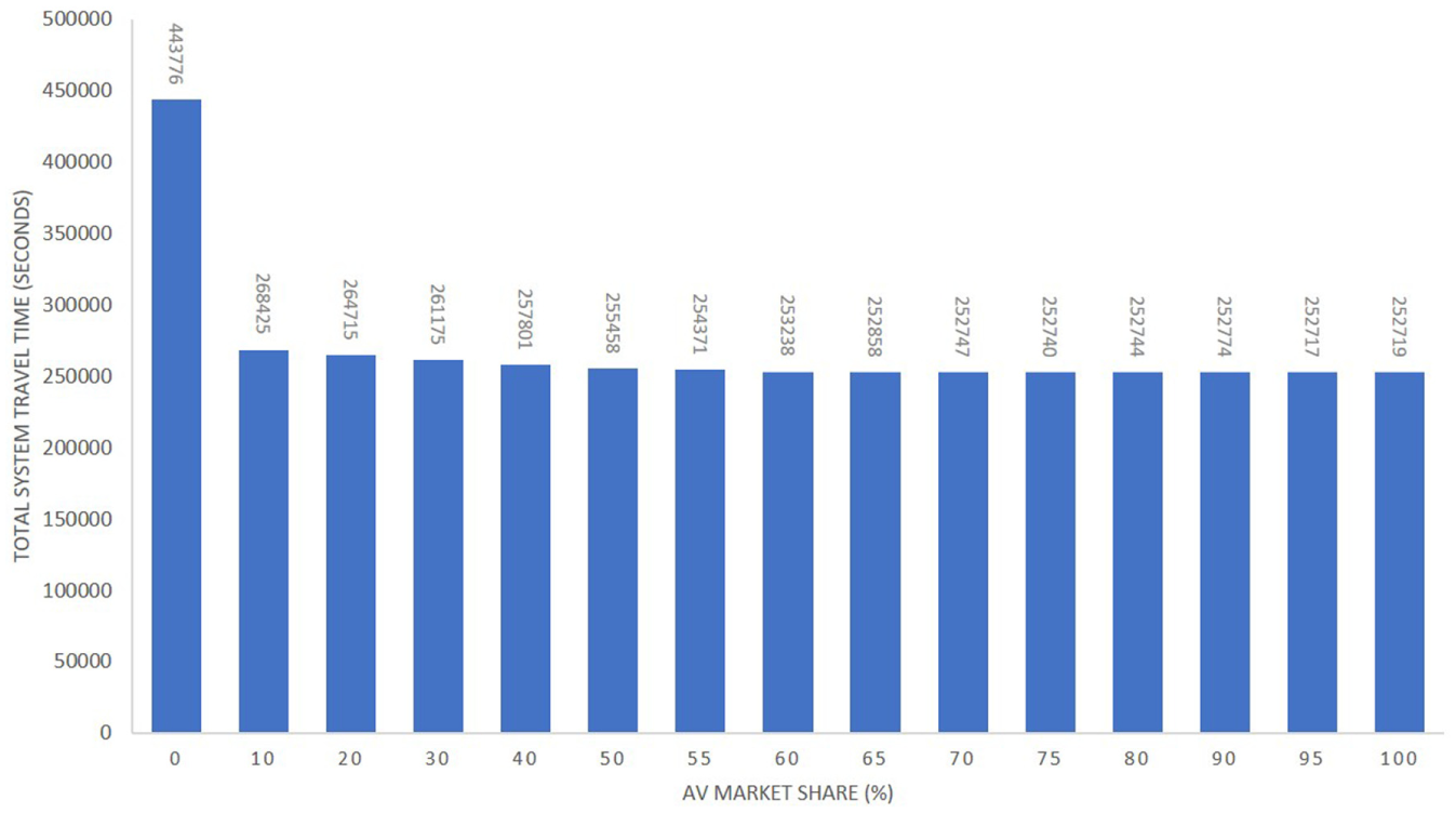
Change in system travel time with different AV market share.
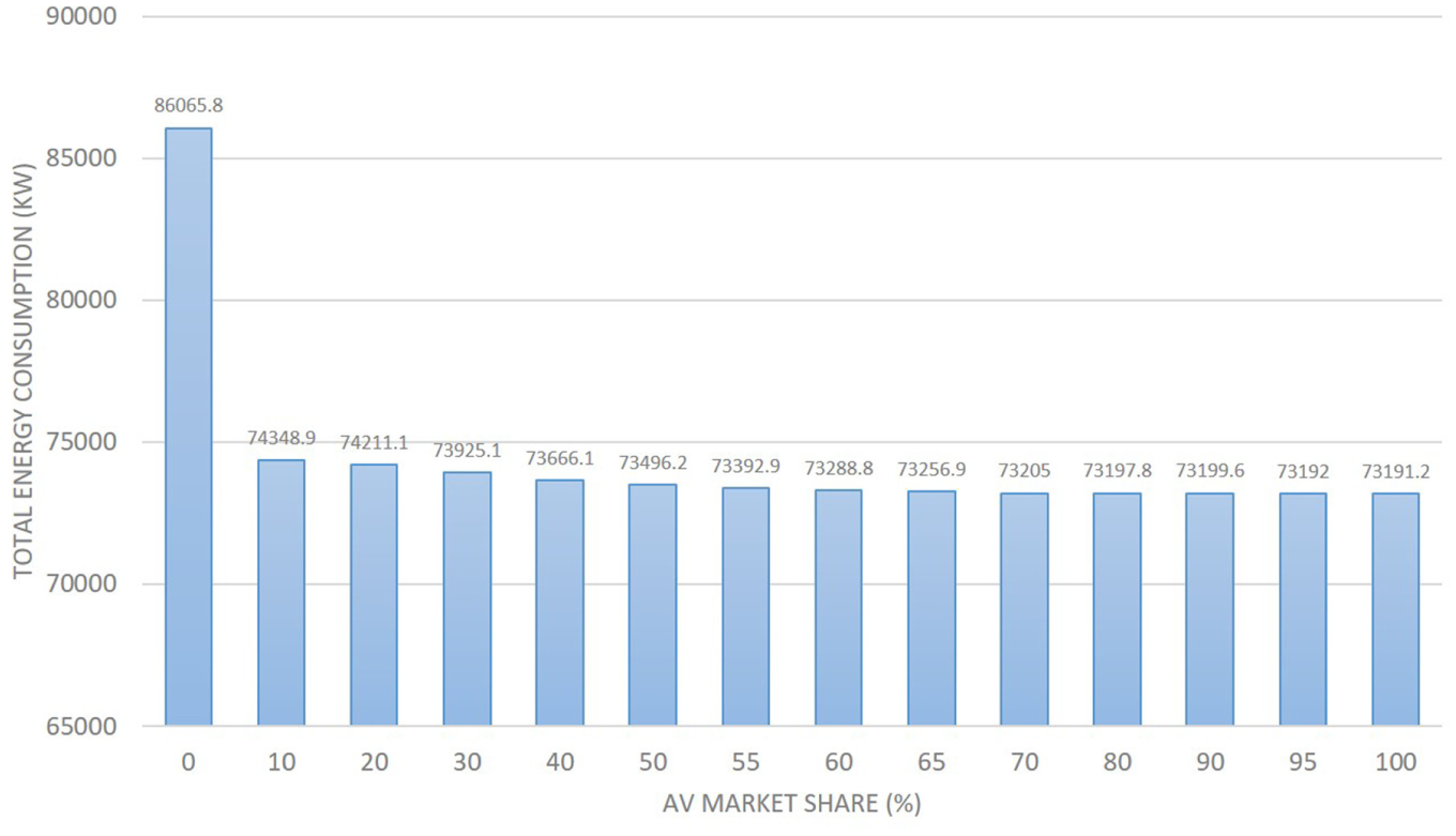
Change in energy consumption with different AV market share.
Flow Distribution at the Path Level
The system optimal DTA model keeps redistributing the flows as the AV market share in the network is increased. Figure 12 illustrates flow redistribution for a single O-D among its three paths. It is obvious that the AV flow share will increase with the AV market share. Nevertheless, the pattern is not identical across the three paths. For instance, the DTA solution assigns higher AV flow to Path 1 (which is, distancewise, the longer path) than to the other two paths. Higher AV flows will help to attain higher density, resulting in maximal throughput and minimal system travel time. It is possible that the system optimal DTA model will assign more AV flows to the path which is longer (distancewise) to have a faster flow propagation.
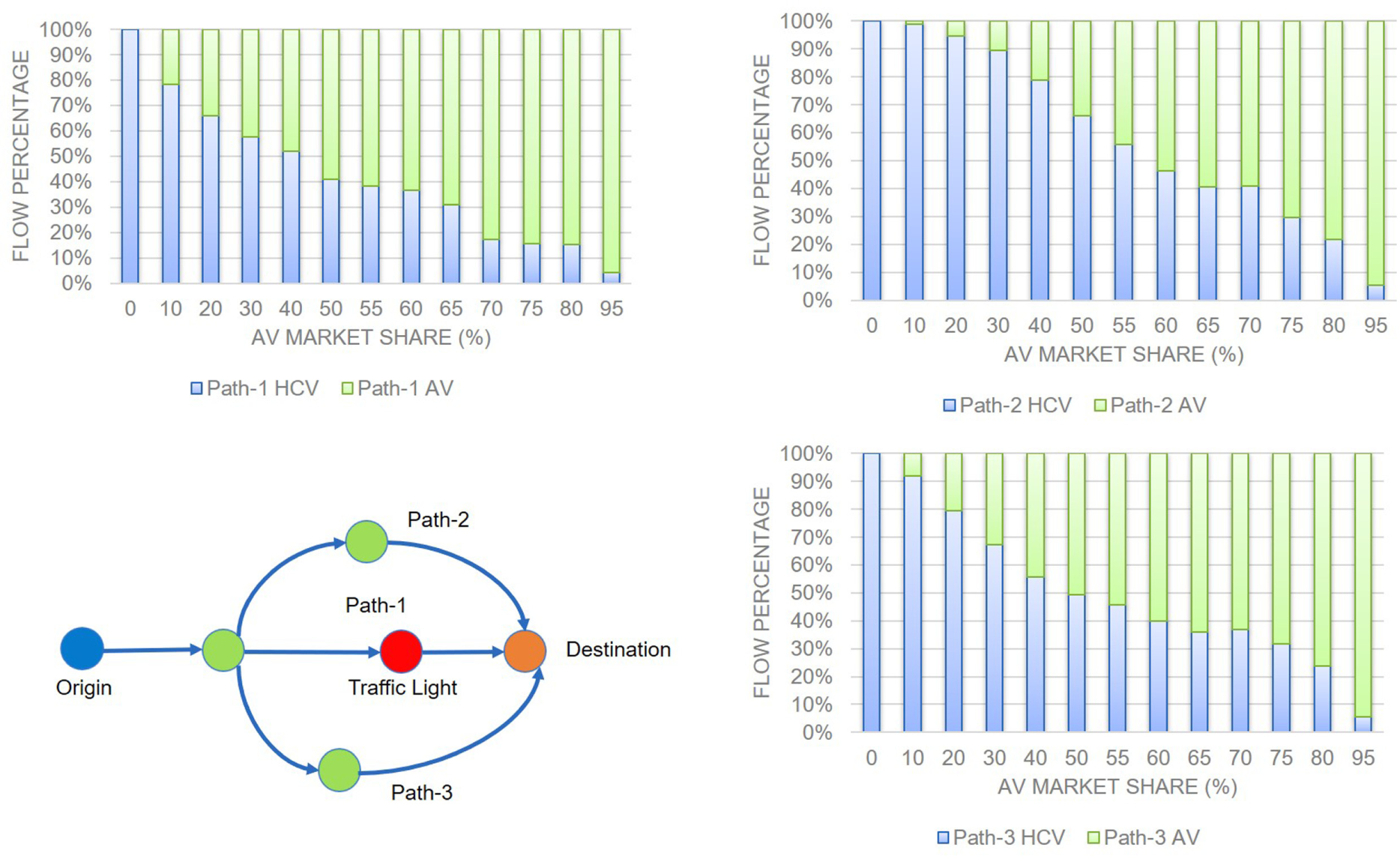
Flow redistribution from system optimal DTA solutions with different AV market share (for clarity, only the O-D pair corresponding to the results is shown at bottom left).
Comparing AV and HCV Average Travel Cost at the Path Level
Further, travel time costs are compared for AV and HCV flows specific to a path to examine the sensitivity to AV market share. Note that for a system optimal assignment the travel cost for certain paths may go up, and this is a well known fact for system optimal DTA solutions. As a comparison with this, a different case is investigated for the same path to find what the (average) cost difference between an AV and an HCV (legacy) is as the market share changes. In other words, the comparison is not between AV and HCV cost among paths, but is rather for the same path. The travel time cost is averaged over all units of flows for the O-D pair specific to a path. In other words, the cost represents the average time to complete the trip for a unit of flow—whether AV or HCV. Figure 13 shows the distribution of cost for different AV shares ranging from 10% to 95%.
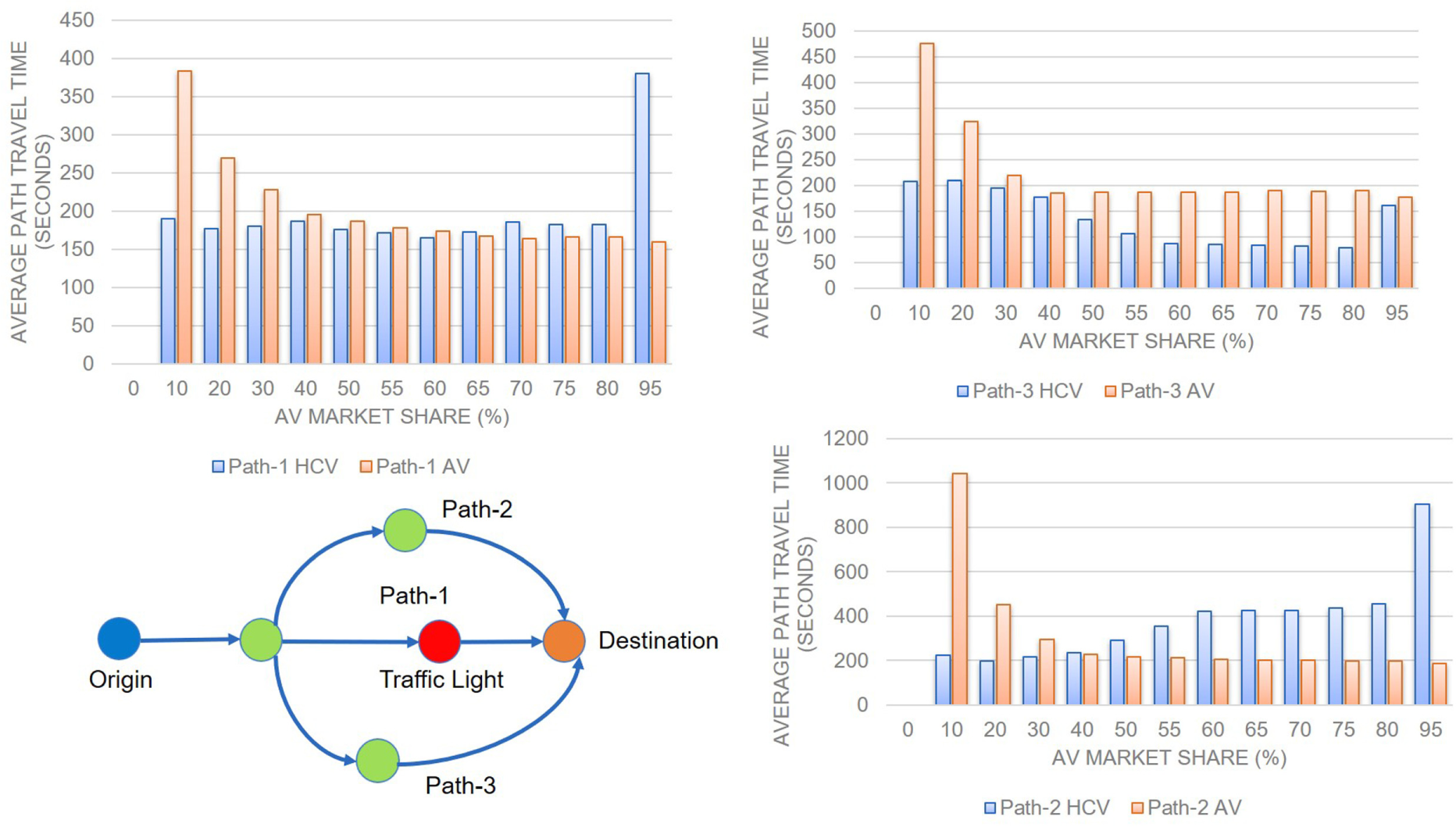
Average travel time cost distribution from system optimal DTA solutions with different AV market share.
For different paths, the pattern is different. Consider the band of 40% to 75% AV share, for which it can be observed that Path 1 has similar average costs for AV and HCV class, Path 2 shows a decrease in HCV average cost with higher AV percentage, and Path 3 shows the opposite pattern to Path 2. Further, for Path 1, HCV cost does not vary much with changes in AV market share except for the high AV market share of 95%. However, AV cost slowly decreases as the AV market share increases. Within the 40% to 80% range of AV share, the costs are similar—not significantly different from each other. For Path 2, HCV cost is always lower than AV cost. In addition, the HCV cost has a significant reduction within the AV share range from 50% to 80%. Further, the AV cost remains almost the same within the 40% to 80% range. For Path 3, the AV cost gets lower and remains almost the same within 50% to 80% range. In contrast, the HCV costs get higher as the AV market share increases.
Effect of Traffic Control
Some experiments were also carried out on the sensitivity of the overall mobility and energy metrics to the existence of a traffic control (Figures 14 and 15). As expected, the travel time and energy impacts are better when there is no traffic light. This scenario could be compared with the case of an automated intersection control where no physical traffic lights exist, and AVs maintain nonconflicting trajectories.
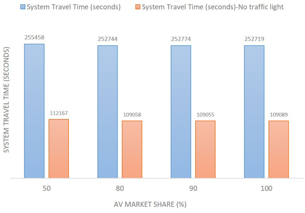
Comparing the travel time impact for traffic control existence.
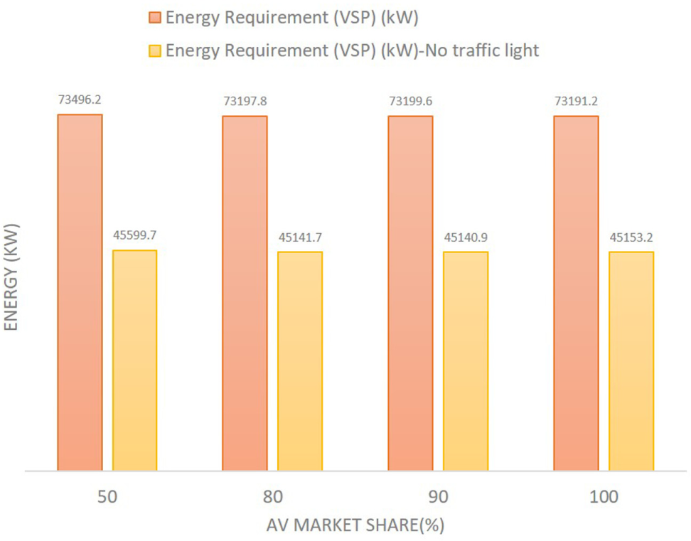
Comparing the energy impact for traffic control existence.
Conclusions and Future Directions
To summarize, the key contributions of this research are as follows: (a) a mathematical program-based system optimal DTA model for transportation networks with mixed traffic flows—AVs and legacy vehicles—was formulated, focusing on mixed density as a function of safe-following distance and PRT, (b) a methodology was developed to estimate energy consumption from spatial-queuing models such as CTMs with approximation of space–mean speed and acceleration values. In addition, the method was validated with data generated from a microsimulation tool, PTV VISSIM, and (c) the mobility and energy impacts of AV market share in a transportation network were assessed.
Key Findings
The key insights from the experimental results are as follows. First, AV deployment in future transportation networks is expected to increase the operational capacity, resulting in a reduction in travel time and energy consumption at the system level. This effect was explained based on traffic flow theory. Results were reported on the benefits of AV market share increment. The results indicate travel time reduction as high as 49% and energy consumption reduction as high as 28% for a test network. Second, an increase in AV market share can cause more travel time at path level on an average for the HCV class using the same path, but for different paths, the pattern is different. For the case of 40% to 75% AV share, AV and HCV classes in Path 1 experienced similar average costs whereas Path 2 shows lower HCV average cost with higher AV percentage. In addition, Path 3 and Path 2 report the opposite pattern in this context. Finally, the distribution of AV and HCV flows among available paths is heterogeneous in nature and may be influenced by factors such as long distance, traffic light existence, and overall capacity of the link.
Findings are similar to those found in some of the recent studies. Rios-Torres and Malikopoulos found that at 100% penetration of CAVs, total fuel consumption decreases by 16% to about 60% and the travel time between 40% and 67% ( 65 ). More results on partial CAV penetration are reported in the paper as well. Elibert et al. analyzed the impact of headway, less braking, and less fluctuation of speed in the context of connected and automated vehicles ( 66 ). They modeled passenger cars on I-91 northbound corridor near Springfield, Massachusetts. The automation is modeled through the CACC Driver model DLL from Turner-Fairbanks Highway Research Center of the FHWA. On average, the maximum benefit reported was in the range of 4% to 5% from the baseline per vehicle. Note that the experimental settings in the study are different from the proposed system optimal dynamic settings. Chen et al. reported the possibility of a 45% reduction in an optimistic scenario ( 67 ). Again, the results do not consider a system optimal dynamic routing. Similar results are reported in the studies by (11, 13). CACC utilizes a concept similar to the smaller headway distribution, and a significant number of studies can be found in the literature (68–70).
Limitations
The model developed here is computationally expensive because of its nonlinear structure and solution techniques. Obtaining solutions for a large-scale network may not be feasible. One potential solution is to apply simulation-based optimization techniques that will render scalability and reduce computational complexity in a significant manner. To have a statistically sound interpretation, it is better to have more than one test network. Nevertheless, the test network used in this study is representative of the general network configurations (e.g., merging, diverging, and traffic lights) and is suitable within the scope of examining the mobility and energy impacts of a system optimal DTA model for mixed traffic of HCVs and AVs.
Implications for Planning and Operations
The system optimal DTA model can provide the upper bounds of energy and mobility benefits for a transportation network with mixed traffic—AVs and HCVs. This is critical from transportation planning and infrastructure investment decisions. As technological progression in AV deployment is observed, it is high time to assess the benefits at the network and regional levels. The macro-level traffic flow model embedded in the DTA model is more computationally tractable than a microsimulation tool with details of car-following behavior. The developed model is expected to assist transportation planning and investment decision processes by quantifying the mobility and energy impacts in future transportation networks with a mixed traffic of AVs and legacy HCVs.
Footnotes
Acknowledgements
The author thanks SMA Bin Al Islam for help with the data generation from VISSIM to validate the energy consumption technique.
Author Contributions
The author confirms sole responsibility for the following: study conception and design, data collection, analysis and interpretation of results, and manuscript preparation.
The Standing Committee on Transportation Network Modeling (ADB30) peer-reviewed this paper (19-04996).
This work does not use any financial support from the Oak Ridge National Laboratory or the U.S. Department of Energy. The results and opinions expressed in this research do not by any means represent any views of the U.S. Department of Energy or the Oak Ridge National Laboratory.