Characterization of Drayage Activities in the Paso Del Norte Airshed

Abstract

The overall objective of the study was to characterize drayage truck activity and associated emissions in the Paso del Norte region, which is the binational region covering El Paso in Texas and Ciudad Juárez in Mexico. Drayage trucks are a significant source of emissions in the Paso del Norte airshed. The region faces air quality problems and characterizing the unique operational and emission characteristics of drayage vehicles can better support regional air quality planning. In this study, the global positioning system and portable activity measurement system units were fitted to a sample of drayage trucks operating in the El Paso region. The resulting data were analyzed to generate trip-level information on truck activity, along with key parameters, such as speeds, origin, destination, and length. The individual trip information was also used to identify key freight corridors and to estimate emissions associated with drayage activity. The study dataset showed that the Ysleta-Zaragoza International Bridge is the most utilized by the trucks. The facilities visited in the United States tended to be more clustered closer to this bridge, in less urbanized areas, while facilities visited in Mexico tended to be more spread out geographically. Corridor truck volumes and emissions were plotted on maps to visualize emission impacts of drayage trucks, with urbanized areas and areas close to border bridges likely most affected because of higher volumes and emissions. The findings from the study provide an understanding of air quality impacts of drayage trucks in the Paso del Norte airshed.

The El Paso area in Texas is part of a larger binational region termed the Paso del Norte, covering parts of Texas and New Mexico in the United States and the city of Ciudad Juárez in Mexico. Air quality is a concern for this binational airshed, with El Paso County in Texas and Doña Ana County in New Mexico in violation of federal ambient air quality standards for particulate matter (PM). Ozone is also a pollutant of emerging concern in the region because of lowered federal ambient air quality standards.

Large volumes of U.S.–Mexico trade pass through the ports of entry (POEs) in El Paso, mostly using short-haul drayage trucks to move goods across the border between intermodal facilities on the Mexican and U.S. sides. Drayage trucks tend to be older and higher emitting than their long-haul counterparts. They are a significant contributor to the emissions inventory in the region, and there is a need to understand better and characterize their activity and emissions. This characterization will help transportation agencies, air quality authorities, and policymakers in developing strategies to improve the air quality of the region.

At present, the relationship between air quality and drayage truck operations is not represented adequately in the emission inventories and travel demand models. However, collecting high-resolution speed and location information from drayage trucks using global positioning system (GPS) units or other devices can improve activity characterization and emission estimates. The overall objective of the study was to characterize drayage truck activity and associated emissions in the Paso del Norte region, which is the binational region covering El Paso in Texas and Ciudad Juárez in Mexico.

Literature Review

Drayage is the dominant practice for goods crossing the U.S.–Mexico border. Drayage trucks, which are Mexican domiciled, are allowed to operate within a zone within 15 mi beyond the El Paso city limits ( 1 ). In areas near the border, such as El Paso, drayage activities can be a significant part of the total freight in the region ( 2 ). Although there have been recent efforts to open the border to more Mexican long-haul trucks, including multiple pilot programs, the drayage system is expected to continue, at least in the short and medium term ( 3 – 5 ).

Figure 1 illustrates the typical drayage process at the U.S.–Mexico border. Usually, the drayage process is considered to start with goods from Mexico being transported to a warehouse on the Mexican side of the border. Here, customs brokers work to get the necessary paperwork and approvals in place, and drayage trucks pick up the goods for shipment. Goods are inspected at both Mexican customs at the border (Aduanas) as well as on the U.S. side by U.S. Customs and Border Protection (CBP). Vehicles may also undergo additional inspections, including safety inspections, during the process. Following this, the drayage truck exits the port of entry and drops goods off at a U.S.-based warehouse or facility. The truck then returns to Mexico, either empty or carrying a return load ( 2 ).

Figure 1.

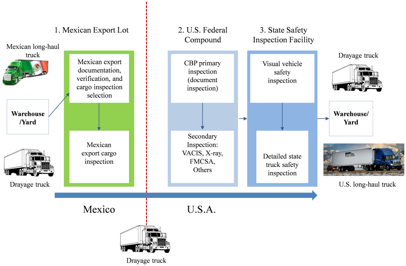
Border crossing process (adapted from [ 6 ]).

Border wait times can sometimes be hours long, so drayage trucks spend much of their time idling, and the trucks do not travel very long distances. Therefore, there is limited incentive for shipping companies to use newer fuel-efficient trucks, and the drayage fleet is typically older than the long-haul fleet. A 2013 study by Farzaneh et al. estimated emissions produced at border crossings by studying a sample of 3,000 vehicles at Bridge of the Americas (BOTA) and the Ysleta-Zaragoza Bridge in El Paso ( 7 ). This study employed the use of GPS data to characterize vehicle activity and emissions, similar to a past study in which vehicle activity data were collected from different classes of vehicles to develop local drive schedules for motor vehicle emission simulator (MOVES) emissions estimation in Texas ( 8 ).

Specifically, for drayage vehicle operations, a recent study focused on characterizing the activities and emissions of drayage truck activities in the Laredo–Nuevo Laredo region. In this study, drayage activities were characterized on both trip-by-trip and link-by-link bases using the GPS data from a sample of trucks. The trip data were used to determine the most visited trucking facilities, and the link summary data was used to develop maps illustrating the key freight corridors in the region ( 2 ). GPS data and data from Portable Activity Measurement System (PAMS) installed on drayage trucks in El Paso were also used to characterize drayage driver behavior and idling ( 9 ).

Several other similar studies have been undertaken by researchers around the United States to characterize vehicle activity and operations and assess the validity of GPS data. Jackson et al. tested two GPS receivers along a 65-mi route from Hartford to Enfield in Connecticut and found that the activity data were comparable to those obtained from onboard diagnostics (OBDs) ( 10 ). Greaves and Figliozzi assessed passive GPS technology for vehicle activity data collection ( 11 ). In this study, the research team installed GPS devices in 30 trucks in Melbourne, Australia, and collected data for a week. Second-by-second truck travel information was used to characterize trip duration, speed, number of stops, and distance traveled. Li et al. applied disaggregated GPS-based technology to collect vehicle activity data in morning commute route choices ( 12 ). The results from these studies show the reliability of GPS data and the ability of GPS to supplement traditional methods of activity data collection (such as vehicle counts) to establish vehicle activity, origins/destinations, and routes.

Also, in the literature, there are multiple studies that characterize the emissions of drayage trucks. A drayage truck’s typical stop-and-go driving cycle contributes to increased emissions with more frequent stops and idling during border crossing times and load/unload periods. Drayage trucks typically make daily trips of fewer than 200 mi and do not idle overnight. While drayage fleets are primarily comprised of small carriers, several carriers dominate the El Paso–Juárez border crossing. A prior study surveyed more than 200 different carriers crossing the border and found that 16 accounted for approximately half of the total trips. Presumably, this translates into a somewhat consistent fleet of trucks crossing the border ( 13 ).

A previous study evaluated drayage idling at both border crossing bridges at El Paso ( 13 ). The main findings of the study indicated that idling and creeping were more than 60% for both bridges. Creep idling, or queue idling, refers to the idling that occurs when trucks waiting in long lines idle and move very slowly. Normal idling occurs when the vehicle is at a total standstill, whereas creep idling occurs when the vehicle is moving at a speed of less than 5 mph and has an acceleration or deceleration of less than 0.5 mph/s. Normal idling is more than creep idling. This normal idling is very significant, because creep idling is very difficult to control, and most idle control technologies are not adequate for creep idling applications. The Ysleta-Zaragoza crossing had higher travel and idling times than the BOTA crossing. The average normal idle time per truck per crossing for BOTA was 9.5 min and 21.5 min for the Yselta-Zaragoza crossing. These higher idling times, in turn, contribute to higher emissions at border crossings ( 13 ).

Several emission testing studies using portable emissions measurement systems (PEMSs) to characterize emissions of drayage trucks and Mexican-domiciled trucks have also been reported. One of the studies indicated that same model year trucks had similar emission profiles in both Mexico and the U.S. ( 13 ). A separate study examining Mexican truck emissions using various types of fuel also found that using Mexican fuel, which has higher sulfur levels than ultra-low sulfur diesel fuel, did not translate into the expected higher PM emissions or increased air toxic levels ( 14 ). Another study evaluated the applicability of three SmartWay strategies (use of lighter trailers, modified driving behavior, and use of diesel oxidation catalysts) for border drayage operations. Carbon dioxide (CO₂), carbon monoxide (CO), oxides of nitrogen (NO_x), total hydrocarbons (THCs), and PM emission rates were measured using two PEMS units. A drive cycle-based analysis was performed using drayage operation speed profiles that were collected using GPS and effectiveness was assessed in reducing emissions. All strategies were found to reduce emissions over baseline conditions, with each strategy having differing impacts on other pollutants ( 15 ). In a 2012 study at Ysleta-Zaragoza port near El Paso, different strategies to reduce PM_2.5 emissions were evaluated using a traffic simulation model. It was found that a commercial vehicle strategy to combine U.S. and Mexican cargo in sections together leads to maximum emission benefits ( 16 ).

Methodology

Instrumentation

Data collection was conducted using two types of technologies, GPS and PAMS devices. GPS devices provide locational information (GPS coordinates) of vehicles, which can be used to derive real-time speeds and accelerations. PAMS devices also record GPS information, but they also log information being reported by the vehicle’s engine over the controller area network (CAN) using the SAE J1939 protocol. In this study, however, the data from both the PAMS and GPS units used in the data analysis were only those that could be obtained from the GPS units (i.e., vehicle coordinates on a second-by-second basis). Thus, the data can be collectively viewed as “GPS data,” despite the two instrumentation types used to collect them. The additional PAMS data, such as engine parameters, were not used in the analyses, although they can be used for other analyses, such as assessment of idling and engine operations ( 9 ).

The loggers used for this project were the QStarz BT-Q1000eX (GPS data logger) and the OBD Mini Logger™ (PAMS) from HEM Data, as shown in Figure 2. Both data loggers record data at a 1 Hz rate (i.e., on a second-by-second basis).

Figure 2.

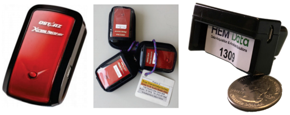
Starz BT-Q10000eX unit (left) and HEM Data Portable Activity Monitoring System (PAMS) data logger (right).

The data collection procedures involved the installation of GPS or PAMS units on participating vehicles, the collection and downloading of data, and the removal of the devices after the data collection period. Data from each unit were downloaded into an electronic spreadsheet, saved onto a central server, and given a unique identifier. After completing the transfer of the data to the server, the research team cleared the data from the data logging units. The number of days and trucks measured are summarized in Table 1.

Table 1.

Summary of Collected Data

Equipment	No. of trucks	No. of days	No. of data points
GPS	26	128	1,865,398
PAMS	4	119	1,780,544

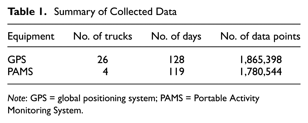
Note: GPS = global positioning system; PAMS = Portable Activity Monitoring System.

Data Analysis Process

Figure 3 shows the data analysis process, and each step is described in further detail in the following sections.

Figure 3.

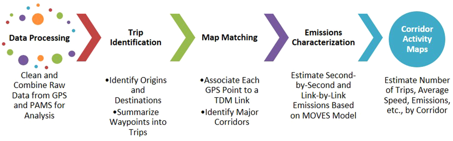
Data analysis process.

Data Processing

Data processing refers to the steps taken to combine and clean the raw data for analysis. The raw data from both PAMS and GPS instruments came as individual files for each truck and day.

Trip Identification

This step involved identifying waypoints and summarizing them into trips. Waypoints were identified by sorting each of the coordinates collected for the single truck by time stamp. Texas A&M Transportation Institute (TTI) researchers imported the specific locational coordinate (latitude/longitude) from the cleaned dataset into the Environmental Systems Research Institute (ESRI) ArcMap GIS software. The spatial join tool in the software was used to assign the following information to each data point: (a) whether the point was located within 1,000 m of a border facility; and (b) the country associated with the point (Mexico or the United States). Then, different trips for each truck and each day were identified using an algorithm, as shown in Figure 4. Trips were defined as periods of activity that had continuous truck movement/activity and that had a distinct origin and destination. The algorithm processed the waypoints on a second-by-second basis and marked the destination if a set of conditions was fulfilled. The conditions used in the algorithm were as follows:

the truck has come to a stop (speed <5 mph) for 5 min continuously;

the truck is not in the proximity of the border crossing (1,000 m);

the truck is at least 1.5 mi from where it originated.

Each truck trip was given a unique identification number, and the data points were converted to a single polyline shapefile containing the complete path of each truck trip. If the trip origin and destination were in different countries, they were classified as cross-border trips and divided into northbound trips (originating from Mexico and ending in the United States) and southbound trips (originating from the United States and ending in Mexico). All other trips were collectively identified as non-cross-border trips.

Figure 4.

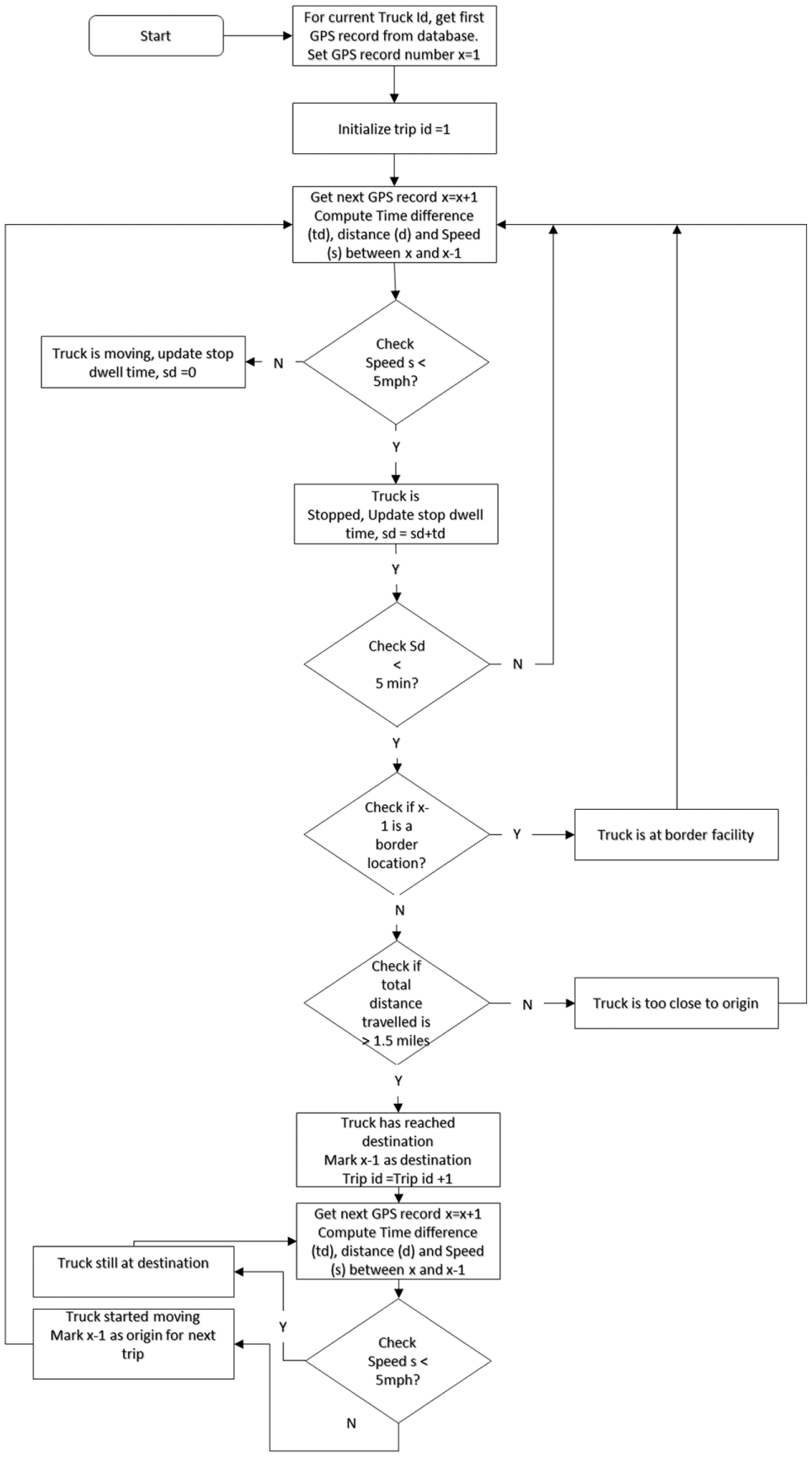
Algorithm for trip identification.

The locations of origins and destinations were also tagged with unique identifications and stored in a data table. Each of these trips was divided into two portions, indicating the trips occurring in the US and Mexico. For each of these portions, average speed and trip length were computed. Data for each unique truck trip (including U.S. and Mexican portions of the trip) and origin and destination locations were then exported to Microsoft Power BI^® software to calculate summary statistics and create graphs for visualization. The trip origins and destinations were also mapped using the ESRI ArcGIS platform. Origins and destinations within the El Paso metropolitan planning area were also linked to traffic analysis zones (TAZs) defined in the Travel Demand Model (TDM) using the spatial join feature.

Figure 5 shows the locations of all the facilities the trucks visited (including both origins and destinations) during the study period (indicated by black dots), with the size of the circles representing the number of trips originating from them. The types of facilities represented are the El Paso airport, offices, warehouses, parking yards, and stores. On the El Paso side, the facilities are concentrated near the Ysleta-Zaragoza International Bridge, which is a designated foreign trade zone of the City of El Paso. On the Juárez side, the facilities are more widely distributed in the commercial and industrial zones of the city. In addition, the facilities on the Mexican side are mostly industrial or manufacturing and the U.S. facilities are warehousing and distribution.

Figure 5.

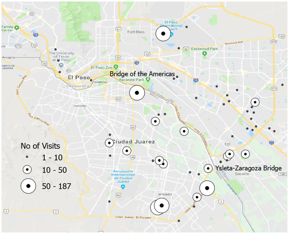
Locations of facilities and number of visits.

Map Matching

Map matching is the process by which the trip data were used to create maps illustrating the movement of trucks along freight corridors in the region. Map Matching involved the following steps.

Step 1—Firstly, waypoints associated with all the trips derived from the study were plotted in ArcGIS and overlaid on TDM links of the region. This plot was used to determine all the corridors used by the trucks during the study period. These corridors were designed to be simplifications of the underlying road network. Each corridor segment was assigned a unique numbered ID. For example, a single corridor was used to represent the path of trips traveling in opposite directions of the same road link. Similarly, single corridors were created to represent major arterial and parallel service roads that were often used by the trucks, or areas around border locations where trucks often took different paths through customs areas.

Step 2—ArcGIS’s spatial join tool was used to associate each GPS point (tagged with GPS unit and trip IDs) with the closest corridor segment defined in Step 1.

Step 3—The resulting data were grouped by corridor ID to obtain a summary of the average speed, the number of discrete truck trips, and the number of GPS points that were joined to each corridor segment. This summary was further disaggregated to derive the average speed and volume of trucks operating on each link during each hour of the day (i.e., midnight–1:00 a.m., 1:00–2:00 a.m., 2:00–3:00 a.m.).

Step 4—These steps were repeated for different time periods within the overall study period to distinguish results for weekdays (Monday–Friday) and weekends (Saturday only) by time of day—morning peak (8:00–10:00 a.m.), midday (10:00 a.m.–4:00 p.m.), evening peak (4:00–7:00 p.m.), and overnight (4:00 p.m.–8:00 a.m.). ArcGIS was used to create maps that plotted the width of the corridor segments as a function of the number of discrete truck trips that occurred on that corridor segment (corridor activity maps). These maps were also used to simultaneously display the average speed and estimated emissions associated with the truck activity on each corridor link.

Emissions Characterization

The summarized truck activities from the analysis were done in two distinct formats—by trip and by link—and emissions were estimated for each of the datasets. The Environmental Protection Agency’s (EPA’s) MOVES emissions model was used to generate emission factors. The MOVES model was used to generate the emission rates specific to the El Paso region considering project-level site characteristics. The pollutants of interest in this study were ozone precursors (volatile organic compounds [VOCs] and NO_x) and PM₁₀. In the emissions analysis, THCs were reported instead of VOCs. THCs included methane, ethane, and acetone in addition to VOCs. However, for vehicular exhaust, these compounds constituted only a fraction of the THCs. MOVES 2014 was used to create a database of NO_x, THC, and PM emission rates specific to diesel short-haul combination truck types operating in El Paso to represent drayage trucks. These MOVES emission rates, expressed in grams per mile per vehicle (g/mi) were generated for 16-speed bins from <2.5, 5, 10, and every 5 to 75 mph. Also, a database of second-by-second emissions by operational mode (OpMode) bin was created to estimate trip-level emissions.

To calculate trip emissions, the second-by-second emission rates based on different OpModes of the vehicles were used to calculate the emissions at each data point. Then the emissions were aggregated by summing up emissions from all the points for each trip ID during different times of the day (morning peak, midday, evening peak, and overnight), weekday type (weekday or weekend), and activity type (cross-border or non-cross-border).

Calculating emissions for links/corridors involved the following steps.

The average speed of all trucks using the link was used to identify the appropriate MOVES emission rate (g/mi) from the rates derived previously. Because each link consisted of truck volume and speed estimates for each hour of the day, the appropriate emission rates were calculated for each hour of the day (i.e., 24 times).

The total emissions per link (in grams per mile) were calculated by multiplying the emission rate by some trucks using the link during each hour of the day. Total emissions per hour per link were also calculated by multiplying the emission rate per link by the length of the link (emissions in grams per hour).

Finally, total daily emissions per link were calculated by summing up the hourly link emissions. Because of differences in the length of each corridor link, total emissions per mile were used to allow emissions to be adequately visualized in the final maps.

Results

Trip Characteristics

Trip summaries of all the drayage activities during the study period aggregated by type of trip and origin country are shown in Table 2. In total, 468 distinct trips were made during the entire study period. The number of trips originating from the U.S. and Mexico was similar. Most of the trips from Mexico started during morning hours. However, the trips from the U.S. started during the evening. This may be because most of the drivers and the garages of the drayage agencies are on the Mexican side of the border. Also, 244 (52%) of the 468 total trips were cross-border trips. Over the duration of the study, there were 224 non-cross-border trips (48% of the total). Similarly, 67% of the total miles driven during the study were during cross-border trips compared to only 33% of the total miles driven during non-cross-border trips, reflecting the generally smaller average trip length of non-cross-border trips (Figure 6). In total, cross-border trips generated approximately 65% of total NO_x and PM emissions. Southbound cross-border trips tended to occur at higher average speeds in Mexico, while the northbound trips had higher average speeds in the United States. This may be because southbound trips occurred more frequently in the afternoon, possibly coinciding with lighter traffic on the Mexican side (both at the border and on the broader network). Counterintuitively, trucks traveled at lesser speeds during non-cross-border trips than during cross-border trips.

Table 2.

Trip Details and Emissions Estimates

	Cross-border trips
	Northbound			Southbound			Non-cross-border trips			All trips
No. of trips	122			122			224			468
Percentage of total trips	26%			26%			48%			100%
Distance and speed
Country	U.S.	Mexico	Total	U.S.	Mexico	Total	U.S.	Mexico	Total	U.S.	Mexico	Total
Total distance traveled (mi)	1,361.2	1,455.3	2,816.6	1,566.5	1,537.2	3,103.7	1,117.9	1,772.8	2,890.7	4,045.6	4,765.3	8,810.9
Average speed (mph)	20.8	9.0	12.4	11.8	16.9	13.9	17.9	9.0	11.1	16.8	11.6	14.2
Total emissions (all trips)
Total NO_x (g)	19,865.3	29,884.8	49,749.4	24,818.1	27,118.7	51,936.8	16,883.8	35,679.9	52,563.8	61,567.2	92,683.5	154,387.2
Total PM (g)	948.2	1,596.0	2,544.2	1,211.8	1,394.7	2,606.5	854.8	1,954.1	2,808.9	3,014.8	4,944.8	7,965.3
THC (g)	2,663.5	1,333.7	3,997.3	1,736.7	2,238.4	3,975.1	1,211.7	3,148.6	4,360.3	4,282.1	8,050.5	12,332.6

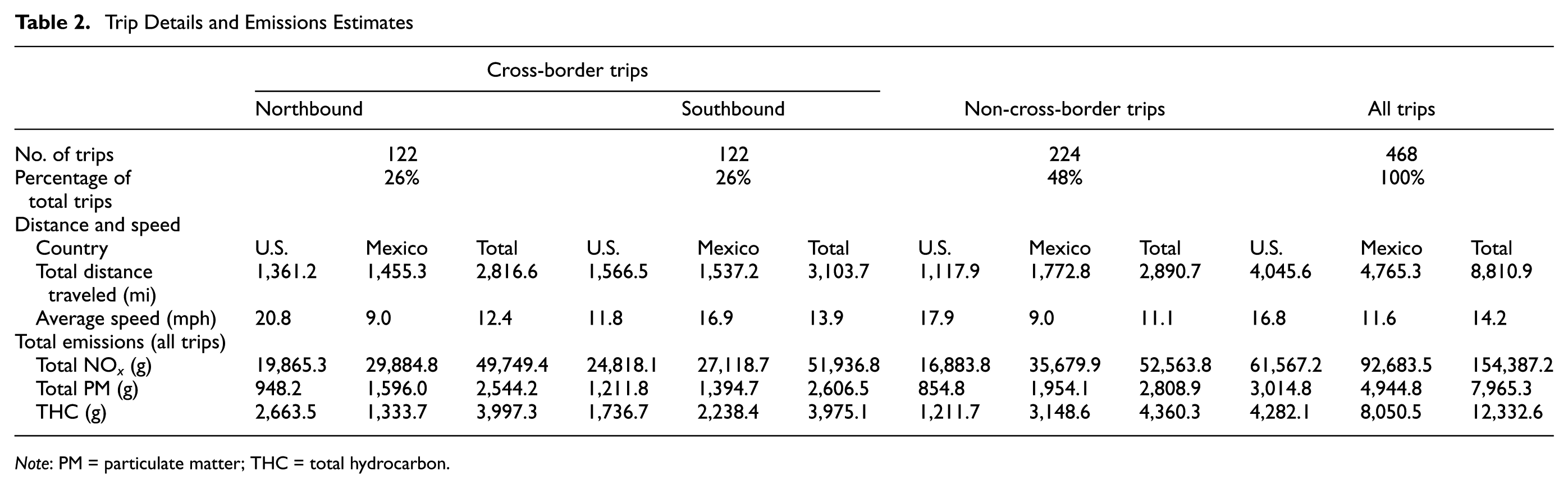
Note: PM = particulate matter; THC = total hydrocarbon.

Figure 6.

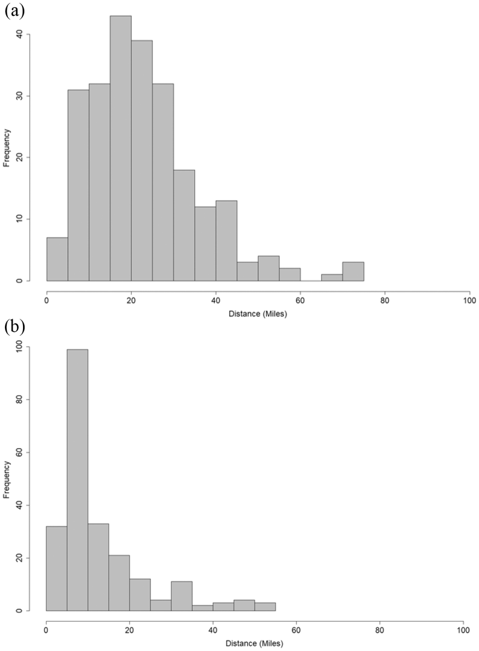
Frequency distribution of trip distances: (a) cross-border; (b) non-cross-border.

Table 2 also shows the total distance, average speed, and emissions generated during travel within Mexica versus the United States. The total distance traveled in Mexico was 18% more than the distance traveled in the United States. As a result, more NO_x and PM emissions were generated in Mexico compared to the United States. However, because trucks generally traveled at a higher speed in the United States than in Mexico (16.8 compared to 11.6 mph, respectively), the emissions were disproportionately higher, with NO_x emissions in Mexico 50% greater than those generated in the United States, while Mexican PM emissions were 64% higher than those emissions generated in the United States.

Figure 7 shows the trends of average distance, average speed, and average emissions of all the trips at different times of day for all the cross-border trips. Northbound cross-border trips (i.e., trips originating from Mexico) were more frequently undertaken in the morning and midday, while southbound trips were more frequently undertaken during the evening and overnight periods. Figure 8 describes the activity and associated emissions during weekdays and weekends for the cross-border trips. More activity and emissions were recorded for southbound trips than northbound trips during weekends. During weekdays, the trend was reversed.

Figure 7.

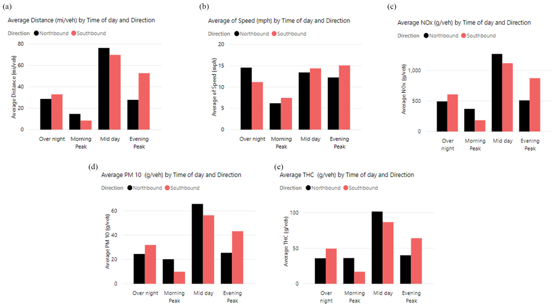
(a) Average distance (mi/veh), (b) average speed (mph), (c) average NO_x emissions (g/veh), (d) average PM10 emissions (g/veh), and (e) average total hydrocarbon (THC) emissions (g/veh) at different times of day (morning peak, midday, evening peak, overnight) for cross-border trips (both northbound and southbound).

Figure 8.

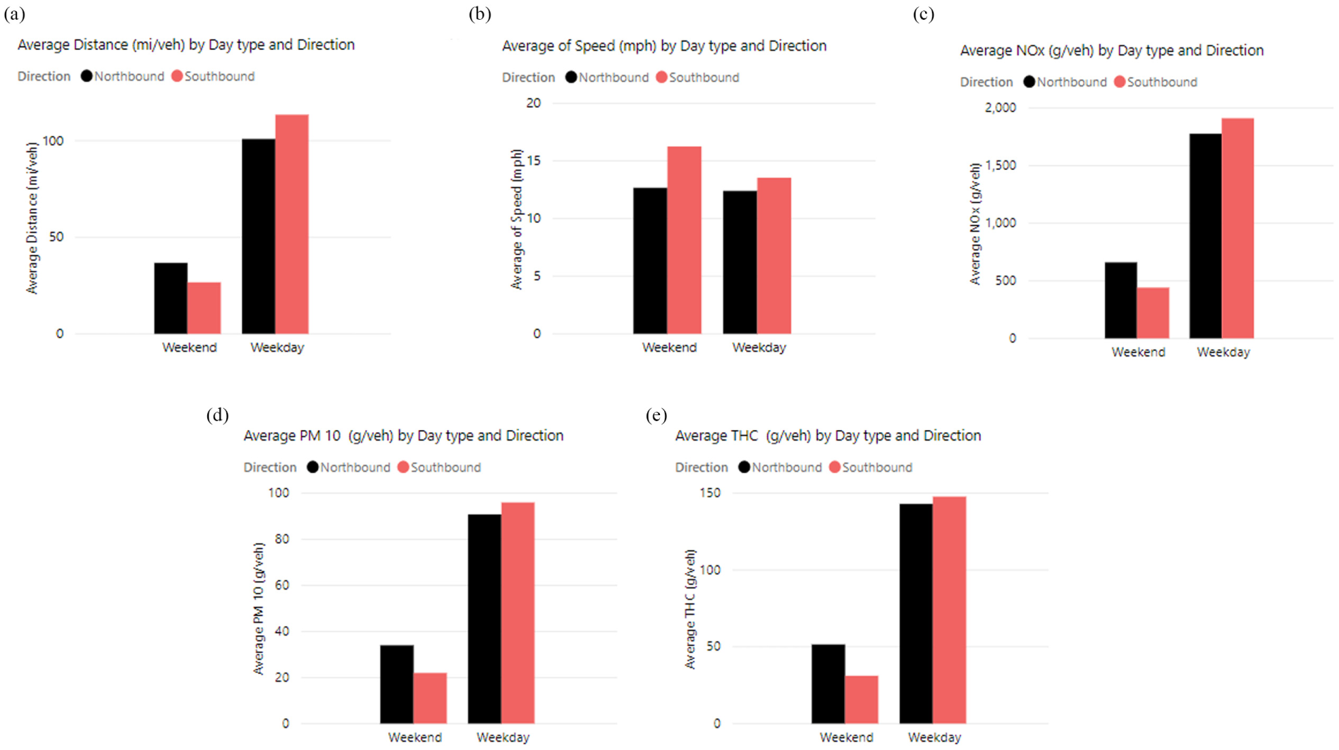
(a) Average distance (mi/veh), (b) average speed (mph), (c) average NO_x emissions (g/veh), (d) average PM10 emissions (g/veh), and (e) average total hydrocarbon (THC) emissions (g/veh) on different day types (weekday and weekend) for cross-border trips (both northbound and southbound).

Figure 9 shows the trends of average distance, average speed, and average emissions of all the trips at different times of day for all the non-cross-border trips. More activity and emissions for non-cross-border trips were on the Mexican side than the U.S. side. Figure 10 describes the activity and associated emissions during weekdays and weekends for the non-cross-border trips. Most of the activity occurred during the weekdays, and the distance traveled and emissions associated were again higher on Mexican side than the U.S for both day types.

Figure 9.

Figure 10.

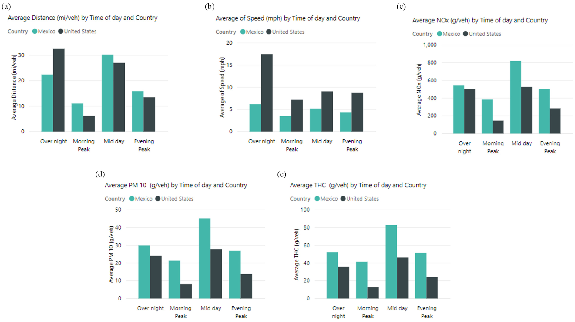
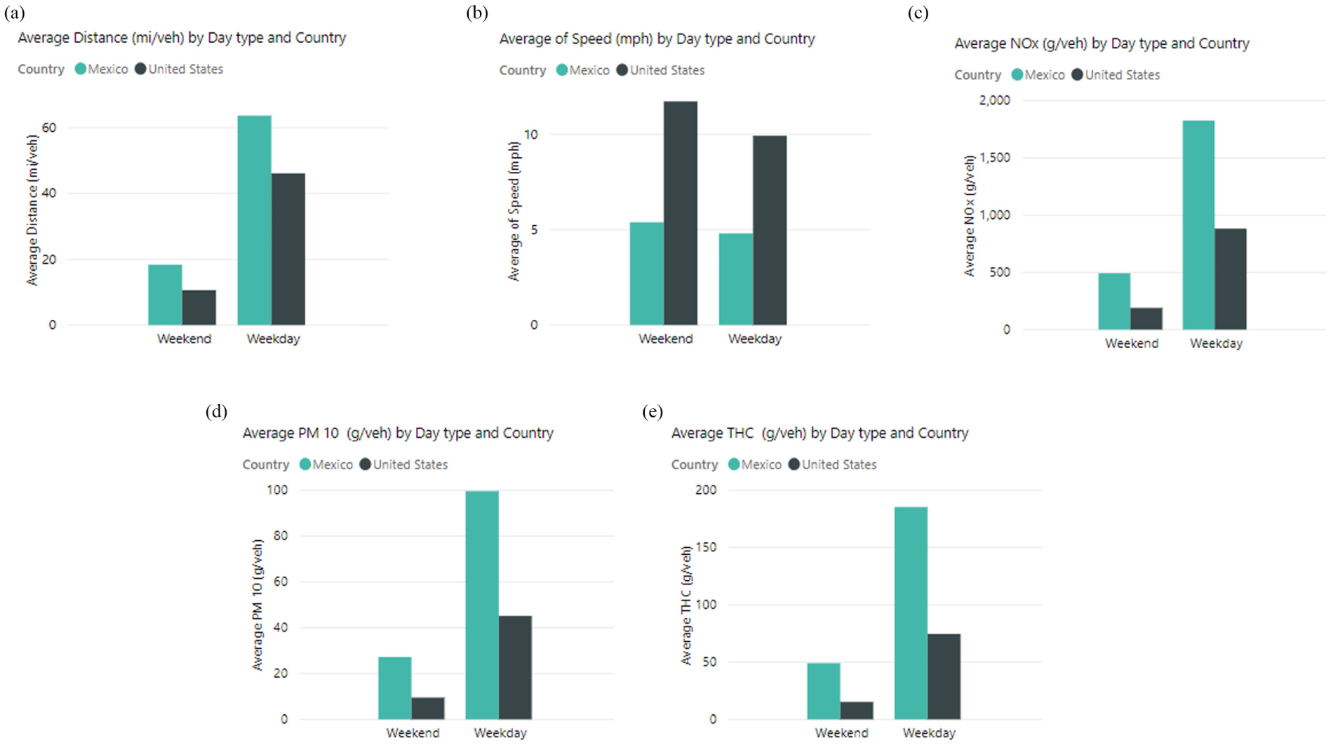
(a) Average distance (mi/veh), (b) average speed (mph), (c) average PM₁₀ emissions (g/veh), (d) average NO_x emissions (g/veh), and (e) average total hydrocarbon (THC) emissions (g/veh) on different day types (weekday and weekend) for non-cross-border trips—United States and Mexico.

The number of northbound and southbound cross-border trips that occurred throughout the study is equal. This finding reflects the reciprocal nature of drayage activities (i.e., that trucks crossing the border one way will return across the border in a relatively short period [within a single day]). However, a high proportion of non-cross-border trips were also observed. It is likely that delays at the border represent a significant portion of the time taken to complete a cross-border trip, and that non-cross-border trips are used to consolidate goods from some locations on one side of the border before they are delivered to one, or some, facilities across the border.

The differences in miles traveled, speed, and emissions illustrated by these results can be explained mainly by differences in the location of facilities in the United States versus Mexico (Figure 5). Here, two factors are essential. Firstly, the average distance between facilities most likely has a significant impact on the distances traveled in the United States and Mexico for all trips (cross-border and non-cross-border). In general, Mexican facilities tend to be more widely distributed than U.S. facilities. Secondly, the distance traveled during cross-border trips is also likely related to the distance between border crossings and each facility. Again Figure 5 illustrates that the most frequently visited U.S. facilities tend to be located much closer to the frequently used Ysleta border crossing, compared to facilities in Mexico.

Corridor Activity and Emission Maps

The complicated relationship among travel distance, travel speeds, and emissions highlights the importance of developing a thorough understanding of the truck activity on the network. This section provides maps illustrating the volume, speed, and emissions of trucks using the network according to different aggregations of trip type and period. In all cases, the width of the bands represents truck volume, and the color of the lines represents either speed or the emissions per mile (PM, NO_x, or THC) calculated using truck volumes and average speeds.

Figure 11 provides an illustrated map of truck volume and speed for the entire study period. The width of the corridors represents the truck volume and the color of the corridors represents the speed of the trucks. For the same period, Figure 12 shows the NO_x emissions associated with the speed illustrated in Figure 11. The maps illustrate that the most critical crossing location throughout the study was the Ysleta bridge, and as might be expected, there is an approximately 1-mi stretch of the network on either side of the crossing associated with high truck volumes, low speeds, and therefore high and concentrated emissions. Figures 11 and 12 also illustrate the generally longer travel distances and lower travel speeds in Mexico compared to the United States. Of particular interest is the proximity of the Ysleta crossing to the most densely urbanized areas of El Paso and some facilities in this area. Emissions close to the U.S. border tend to be highly concentrated because of relatively slow speeds associated with the border crossing and the urban roads close to the border.

Figure 11.

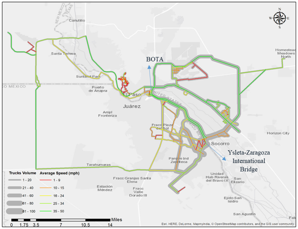
Overall volume of trucks and average speed (mph). (Color online only.)

Figure 12.

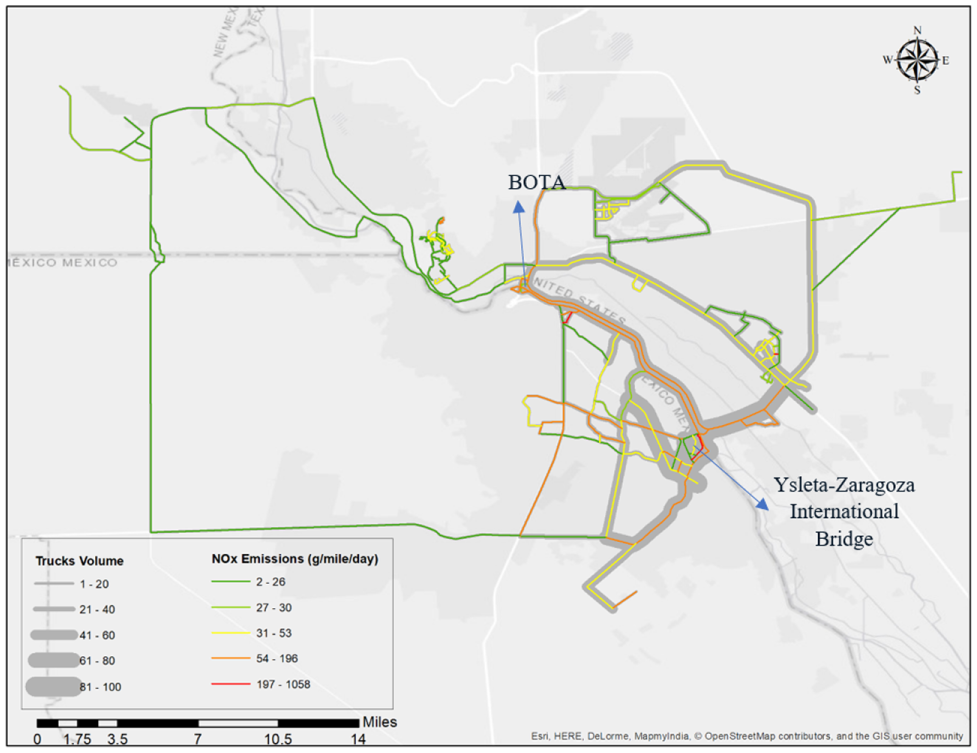
Overall volume of trucks and NO_x emissions (g/mi/day). (Color online only.)

As illustrated in a combination of Figure 5 with Figures 11 and 12, the most heavily visited Mexican facilities are close to urban areas and the border. However, the most densely urbanized areas of El Paso are located farther away from the U.S. facilities and, in general (except for the congested urbanized areas), average speeds on the U.S. network tend to be higher. Another significant feature of Figure 11 is the relatively low volumes of trucks using the Bridge of the Americas to the west of El Paso relative to the Ysleta-Zaragoza Bridge. This phenomenon is somewhat anomalous given that BOTA has higher volumes of commercial vehicles crossing than does the Ysleta POE overall. This observation is likely a function of the particular shippers and their route preferences in the dataset and cannot be considered indicative of the drayage vehicle movement in El Paso as a whole.

Conclusion

The overall objective of this study was to characterize the activities and emissions of drayage trucks in the Paso del Norte region. This is an important area of investigation given the current concerns with ambient air quality in the region and the potential impacts on human health. El Paso is one of the busiest POEs for trucks entering the United States from Mexico, and past studies have established the significant contribution of drayage trucks to the overall emissions inventory in the region.

This study successfully collected data and implemented analytical methods to characterize drayage truck activity and emissions. The study findings provide insight into several topics, including the following.

Use of high-resolution data for activity and emissions characterization: Use of GPS and PAMS data collected on a second-by-second basis allowed for the assessment of vehicle activity and emissions characteristics at the link level and individual vehicle trips.

Understanding drayage activity patterns: Morning and midday drayage activities generally occurred on the Mexican side of the border, likely because of drayage companies being Mexican domiciled. Similarly, evening and overnight activities tended to involve return trips from the United States to Mexico. The timing of the return trips seemed to be more varied and may be because of drivers or companies aiming to bring reciprocal loads back to Mexico rather than returning empty. Similarly, weekend activity was very limited relative to weekdays.

Importance of non-cross-border trips: The study results showed that non-cross-border trips are frequent and an essential part of drayage activities. These trips are of shorter distance and duration and are likely undertaken by drivers commuting home in work trucks or seeking to consolidate loads before the border crossing process.

Drayage vehicle routes: In the dataset from the study, it was seen that the location of different facilities visited by the trucks varied spatially on both sides of the border. Most of the U.S. facilities visited are located close to the Ysleta- Zaragoza POE, while the Mexican facilities are more widely distributed. This could explain why the majority of the border crossings in this study took place at the Ysleta-Zaragoza POE, despite BOTA being the bridge with higher commercial vehicle volumes overall.

Potential emissions impacts: The slow speeds associated with border crossing, in combination with lower speeds within urban areas, lead to high emission concentrations in this area. The location of residential areas near these border crossings may, therefore, result in public health impacts because of congestion and emissions.

The findings from this study provide several insights into drayage vehicle activities and emissions from the Paso del Norte region. While the study included a large dataset of drayage vehicles (over 200 truck-days of operational data from three companies), additional data from a larger sample of trucks could further supplement these findings. The current dataset could have sampling bias, as the drayage companies selected for the study may have particular route choices and operating hours compared to other companies in the area. Applying the methodology on a larger dataset could include identifying a more extensive range of origins/destinations and route choices. Further information on the types of loads carried, whether trucks are equipped with refrigerated units, and other details can help improve emissions characterization. Additional factors not considered in this study that may affect cross-border activities and route choice include the impact of the volume of non-commercial traffic on the network or real and perceived border wait times at different bridges.

In conclusion, this study developed and implemented data collection methods and analyses to characterize drayage truck activities in the Paso del Norte region. The study findings can be used to explain the drayage activities and their air quality impacts to a broad range of border transportation stakeholders, and to support regional air quality and transportation planning.

Footnotes

Acknowledgements

This work was performed by the TTI for the El Paso Metropolitan Planning Organization (MPO) and was funded through a State and Local Air Quality Planning Program grant from the Texas Commission on Environmental Quality (TCEQ). The authors would like to acknowledge the contributions of the following TTI researchers: Andrew Birt for guidance on data analysis, Chaoyi Gu for assistance with emissions rates, and Lorenzo Cornejo for assistance with data collection. The authors would also like to thank Claudia Valles and Michael Medina of the El Paso MPO for their input and oversight.

Author Contributions

The authors confirm contributions to the paper as follows: study conception and design: RF, JJ; data and information collection: RF, JJ; analysis and interpretation of results: RJ, RF, TR; draft manuscript preparation: RJ. All authors reviewed the results and approved the final version of the manuscript.

The Standing Committee on Transportation and Air Quality (ADC20) peer-reviewed this paper (19-03298).

References

Harrison

Hutson

Prozzi

Mccray

West

The Impacts of Port, Rail, and Border Drayage Activity in Texas. FHWA/TX-09/0-5684-1. Texas Department of Transportation, Austin, 2009.

Birt Farzaneh

Johnson

Overmyer

Zietsman

J. A.

Characterizing Drayage Activities and Emissions in the Laredo-Nuevo Laredo Airshed. Texas A&M Transportation Institute, 2016.

Federal Motor Carrier Safety Administration. United States to Expand Trade Opportunities with Mexico through Safe Cross-Border Trucking. https://www.fmcsa.dot.gov/newsroom/united-states-expand-trade-opportunities-mexico-through-safe-cross-border-trucking.

Birt

Ramani

Farzaneh

Zietsman

Emissions from Long-Haul Mexican Diesel Trucks in the Laredo-San Antonio Corridor. Texas A&M Transportation Institute, College Station, 2015.

Cassidy

Mexican Trucking Past US Border in Crosshairs. Journal of Commerce, 2017. https://www.joc.com/trucking-logistics/truckload-freight/politics-economics-collide-us-mexico-truck-crossings_20170213.html

Villa

J. C.

Development and Implementation of Technology to Measure Truck Crossing Time at International Land Ports of Entry. Archives of Transport, Vol. 34, No. 2, 2015, pp. 75–86. https://doi.org/10.5604/08669546.1169215.

Farzaneh

R. M.

Fossett

Williams

Wood

Zietsman

Developing an Emission Estimation Tool for Border Crossings. Presented at 94th Annual Meeting of the Transportation Research Board, Washington, D.C., 2015.

Farzaneh

Zietsman

Lee

D. W.

Johnson

Wood

Ramani

Texas-Specific Drive Cycles And Idle Emissions Rates For Using With Epa’s Moves Model–Final Report. FHWA/TX-14/0-6629-1. Texas Department of Transportation, Austin, 2014.

Development of Emissions Reduction Program for Heavy-Duty Trucks Operating in the Border Region . Texas Transportation Institute, 2017.

10.

Jackson

Aultman-Hall

Holmén

Evaluating the Ability of Global Positioning System Receivers to Measure a Real-World Operating Mode for Emissions Research. Transportation Research Record: Journal of the Transportation Research Board, 2005. 1941: 43–50.

11.

Greaves

S. P.

Figliozzi

M. A.

Collecting Commercial Vehicle Tour Data with Passive Global Positioning System Technology. Transportation Research Record: Journal of the Transportation Research Board, 2008. 2049: 158–166.

12.

Guensler

Ogle

Analysis of Morning Commute Route Choice Patterns Using Global Positioning System-Based Vehicle Activity Data. Transportation Research Record: Journal of the Transportation Research Board, 2005. 1926: 162–170.

13.

Zietsman

Villa

J. C.

Forrest

T. L.

Storey

J. M.

Mexican Truck Idling Emissions at the El Paso – Ciudad Juarez Border Location. Southwest Region University Transportation Center, Texas Transportation Institute, 2005.

14.

Zietsman

Farzaneh

Storey

Villa

Ojah

Lee

D. W.

Bella

Emissions of Mexican-Domiciled Heavy-Duty Diesel Trucks Using Alternative Fuels. Texas Transportation Institute, The Texas A&M University System, College Station, 2007.

15.

Beard-Raymond

Farzaneh

R. M.

Duran

Zietsman

Lee

D. W.

Johnson

SmartWay Applications for Drayage Trucks. Texas Transportation Institute, The Texas A&M University System, College Station, 2009.

16.

Kear

T. P.

Wilson

J. H.

Corbett

J. J.

United States-Mexico Land Ports of Entry Emissions and Border Wait-Time White Paper and Analysis Template. U.S. Department of Transportation Federal Highway Administration, Washington, D.C., 2012.