Impact of Primary Incident Spatiotemporal Influence Thresholds on the Detection of Secondary Crashes

Abstract

Incident management agencies have been investing substantial amount of resources to devise strategies to mitigate secondary crashes (SCs). Nevertheless, detection of SCs is not a straightforward process, as the definition itself is subjective; identification of SCs depends on how the impact area of the primary incident (PI) is defined. Both static and dynamic methods, the two most common approaches used to define the impact area of the PI, have serious limitations that restrict their practical applications. Although the dynamic method is proven to yield accurate results, applying it requires real-time traffic data which are only available on limited locations. On the other hand, the static method’s one-size-fits-all approach of using fixed spatiotemporal thresholds does not yield reliable results. This study explored the impact of PI spatiotemporal influence thresholds on the detection of SCs. To implement the study objective, both static and dynamic approaches were developed. The static method was based on predefined spatiotemporal thresholds, and the dynamic method was based on prevailing traffic speed data from BlueToad^® paired devices. Comparison of SC frequencies identified using the static and dynamic methods showed that the static method consistently under and overestimated SC frequencies for smaller and larger spatiotemporal thresholds, respectively. The prevailing traffic conditions were found to play a crucial role in instigating SCs, as more than 75% of SCs occurred during congested traffic conditions. Use of varying spatiotemporal thresholds depending on the prevailing traffic conditions is expected to reduce the biases associated with the subjective thresholds used in the static method.

Traffic incidents are the primary source of non-recurring congestion. They frequently affect traffic operations, accounting for more than a half of all urban traffic delays and almost all rural traffic delays ( 1 ). Furthermore, traffic incidents expose other vehicles to the risk of becoming involved in a secondary crash (SC) ( 2 ). SCs are generally considered to occur at the boundaries or within the congested spatiotemporal region that builds up as a result of a prior incident, commonly referred to as a primary incident (PI) (3 –6). Although most studies (3, 4, 6) have identified SCs upstream of the PI, it is possible for SCs to occur on the opposite direction of the PI as a result of the rubbernecking phenomenon (5, 7). Figure 1 explains SCs using a hypothetical example. In this example, a prior traffic incident (crash) occurred on northbound (NB) lanes at 8:33 a.m. This crash, categorized as a primary crash, resulted in a queue backup upstream of the crash location.

Figure 1.

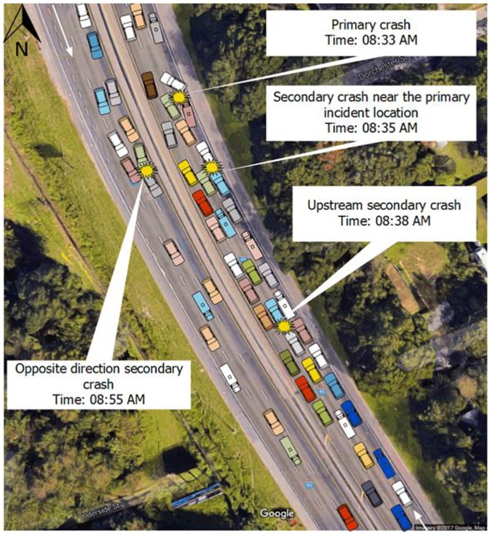
Definition of a secondary crash.

Two crashes, one near the primary crash location and the other further upstream of the primary crash location, occurred at 8:35 a.m and 8:38 a.m., respectively. Another crash also occurred in the opposite direction (i.e., on southbound (SB) lanes) at 8:55 a.m.. The first crash that occurred at 8:33 a.m. is considered as the primary crash, and the remaining three crashes are considered as SCs which occurred as a result of the primary crash. In summary, crashes are considered as SCs if they occur: (a) at the scene of the PI (3, 4); or (b) within the queue upstream of the PI ( 4 ); or (c) within the queue in the opposite direction of the PI as a result of driver distraction ( 7 ).

SCs have increasingly been recognized as a major problem leading to reduced capacity, extra traffic delays, and increased fuel consumption and emissions. SCs are non-recurring in nature; not only do they affect the traffic operations, but they also impose risk on safety of road users. The United States Department of Transportation estimated that SCs alone are responsible for approximately 18% of all freeway traffic fatalities and 20% of all crashes ( 2 ). Further, compared with PIs, SCs have significant impact on traffic management resource allocation (6, 8). Prevention of SCs has therefore been highlighted as a high priority task for traffic incident managers ( 9 ) and transportation management centers (TMCs) ( 2 ). In fact, the Federal Highway Administration (FHWA) uses the reduction of SCs as one of the performance measures for state incident management systems ( 10 ). Several states, including Florida, are considering SC mitigation strategies in allocating funding for on-road help services (e.g., Road Rangers) and the development of traffic incident management programs ( 11 ).

Accurate identification of SCs is crucial to developing their mitigation strategies, as the success of these strategies heavily depends on the knowledge of the inherent mechanisms of when and where SCs occur. However, SC detection is not a straightforward procedure, as the definition itself is subjective.

Existing Methods for Identification of Secondary Crashes

As mentioned earlier, SCs are crashes that occur within the spatial and temporal impact range of the PIs. Unlike other traffic incidents which are easily identified by incident responders, identification of SCs is not clear-cut. Even incident responders on-site or the TMC personnel, who observe traffic through the Closed-Circuit Television (CCTV), cannot accurately identify SCs. This is because the process of identifying SCs varies depending on the spatial and temporal influence area of the PI. It is difficult to determine visually, either directly at the crash site or through the CCTV camera, if the crash is a result of the backup caused by another prior incident. Thus, accurate detection of SCs depends on the reliability of the spatial and temporal information of the prior incident. The first step in identifying SCs is therefore to define the impact area of the prior incident, that is, its spatiotemporal boundaries.

Three major approaches have been used to define the spatiotemporal thresholds of PIs: (1) manual method in which personnel visually identify the impact area of a PI; (2) static method that uses predefined spatiotemporal thresholds; and (3) dynamic approach that uses varying spatiotemporal thresholds based on PI characteristics and prevailing traffic flow conditions. Once the impact area of the PI is defined, the second step is to identify SCs, which essentially include all crashes that occurred within the spatiotemporal boundary of the respective PI. An extensive review of the literature indicated that tremendous efforts have been conducted to identify SCs. The following paragraphs provide more details about the three abovementioned methods that are used to identify SCs. Notably, comprehensive reviews of the static and dynamic methods can be found in Yang et al. ( 12 ).

As the name “manual” indicates, in this method, SCs are manually identified by either the TMC personnel or incident responders. Identifying SCs on a CCTV camera is considered an off-site approach, and identifying SCs on-site by incident responders including police, Road Rangers, and so forth, is considered an on-site approach ( 10 ). The manual method has traditionally been used by agencies to identify SCs. It is simple and does not require any data processing. However, despite being the most commonly used method, it is subjective, unreliable, inconsistent, and random.

The static method identifies SCs based on some fixed spatial and temporal criteria. Crashes that occurred within the spatial and temporal impact range of a PI are identified as SCs. For SCs occurring upstream of the PI, the spatial and temporal thresholds employed by previous studies range from 1 to 2 mi and 15 min to 2 h, respectively (3, 6, 13 –16). On the other hand, SCs occurring in the opposite direction of the PI were identified using different thresholds. For example, Chang and Rochon ( 13 ) identified SCs using a 30-min–0.5-mi threshold in the opposite direction of the PI.

Unlike the manual method, the static method is more reliable simply because it is a function of predefined spatiotemporal parameters. However, the fixed spatiotemporal thresholds used in the static method are subjective and arbitrary ( 5 ). The method incorrectly assumes that all incident types that occur at different traffic conditions, such as congested and free-flow states, have the same effects on the upstream traffic flow ( 17 ). In fact, incidents occurring during free-flow conditions might not have a long-lasting and far-reaching effect compared with the incidents occurring during congested conditions. In addition, severe incidents are associated with longer incident response and clearance times compared with minor incidents. Thus, both spatial and temporal thresholds should vary based on prevailing traffic conditions, geometric characteristics, and certainly incident characteristics ( 17 ).

To overcome the limitations associated with the static approach, recent studies have focused on detecting SCs using dynamic methods that use prevailing traffic flow conditions. Sun and Chilukuri proposed the use of an incident progression curve, a method that uses incident duration to estimate the queue length and thus identify SCs that occurred within the queue ( 18 ). The incident progression curve method indicated a 30% improvement in the SC identification accuracy compared with the static method. Nonetheless, queuing model-based approaches are limited in the establishment of reliable queuing models. In other words, different roadway segments are subject to different queuing formation processes because of their unique traffic, geometry, and incident characteristics.

Several researchers have estimated flexible spatiotemporal thresholds based on the PI influence area using other dynamic methods such as speed contour, automatic tracking of moving jams, vehicle probe data, shock wave principles, and so forth (5, 18 –22). These approaches take advantage of the traffic data retrieved from infrastructure-based traffic sensors. Use of traffic sensor data enables capturing the effects of traffic characteristics (e.g., flow, speed, and density) that change over time and space, and affect the queue formation as a result of the PI. The results from these studies indicate that the proposed dynamic methods provide better accuracy in identifying SCs than the conventional static method ( 23 ).

In summary, the conventional static method that identifies SCs based on pre-specified spatiotemporal parameters has serious limitations as it fails to capture the actual impact range of PIs. Dynamic methods address this limitation by dynamically determining the spatiotemporal thresholds of PIs based on real-time traffic flow characteristics such as speed and density. However, several dynamic methods still face some shortcomings. For example, methods developed based on queue length estimations require detailed queuing information, which is not commonly available (4, 24). The methods proposed using progression curve identify SCs based on an identical progression curve for all PIs, resulting in inaccurate identification of SCs ( 18 ). Furthermore, the speed contour method is limited to identifying SCs that have occurred upstream of the PI and fail to identify SCs caused by rubbernecking in the opposite direction ( 5 ). In this study, the proposed dynamic SC identification method focuses on estimating the impact range of the PI using speed data archived by the BlueToad^® paired devices and identifying SCs occurring within the impact range of the PI. This method aims to better capture the effects of traffic flow characteristics, such as speed, that change over space and time, and affect the queue formation as a result of a PI.

Compared with the static or manual method, the dynamic method is a more advanced and reliable method as it identifies SCs based on traffic flow characteristics. However, the implementation of the current approach depends on the availability of real-time traffic data. The detectors for capturing real-time traffic flow data are mostly available on urban limited access facilities, and thus, the use of dynamic method is limited to only these locations. Moreover, this method is resource and data intensive.

Study Objective

FHWA has established the reduction of SCs as one of the performance measures for incident management programs ( 10 ). Essentially, detection and mitigation of SCs is one of the priorities of TMCs. Although the detection of SCs using historical traffic data can help in producing SC reports, TMC would benefit from an algorithm that will detect SCs in real time. Although the dynamic method is proven to yield accurate and reliable results, applying it requires traffic data which are only available on limited locations. Therefore for practical applications, the static method is still the most viable approach. However, a one-size-fits-all approach of using fixed spatiotemporal thresholds may not yield reliable results. This is because the impact area of the PI heavily depends on the prevailing traffic conditions, that is, uncongested or congested conditions. As such, this study aims to investigate the impact of PI spatiotemporal influence thresholds on the detection of SCs. More specifically, the impact of uncongested and congested times are investigated. This paper also presents a sensitivity analysis of varying spatial and temporal limits of PIs on the detection of SCs. The study results will assist agencies to more accurately identify SCs in real time, and devise strategies to respond to and mitigate SCs.

Data

The study area includes a 35-mi section on I-95, a 21-mi section on I-10, and a 61-mi section on I-295 located in Jacksonville, Florida. In summary, the total study area covers 117 mi. Data used in this study include speed data from BlueToad^® devices and incident data from the SunGuide^™ database, for the years 2015–2017. In addition to these data, Interstate polyline shapefile was extracted from the Florida Department of Transportation (FDOT) Transportation Data and Analytics Office website.

SunGuide^™

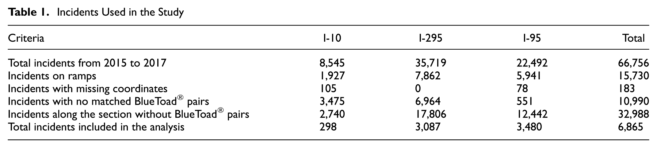
SunGuide^™ is software used for incident management to process and archive incident data. The database stores incident attributes including incident ID, incident timeline, and incident type. Along the study corridors, the SunGuide^™ database included a total of 66,756 incidents from 2015 to 2017. After excluding incidents on ramps (15,730), incidents with missing coordinates (183), incidents with no matched BlueToad^® pairs (10,990), incidents along the section without BlueToad^® pairs (32,988), the remaining data consisted of a total of 6,865 incidents. Table 1 provides more information about the incidents included in the analysis.

Table 1.

Incidents Used in the Study

Criteria	I-10	I-295	I-95	Total
Total incidents from 2015 to 2017	8,545	35,719	22,492	66,756
Incidents on ramps	1,927	7,862	5,941	15,730
Incidents with missing coordinates	105	0	78	183
Incidents with no matched BlueToad^® pairs	3,475	6,964	551	10,990
Incidents along the section without BlueToad^® pairs	2,740	17,806	12,442	32,988
Total incidents included in the analysis	298	3,087	3,480	6,865

BlueToad^® Devices

BlueToad^® devices are Bluetooth signal receivers which read the media access control (MAC) addresses of active Bluetooth devices in vehicles passing through their area of influence. These devices act in pairs or network by recording the time when a vehicle passes both devices. This information is used to deduce travel time of the vehicle between a pair of devices. The speed is calculated from the obtained travel time and a known path distance (not Euclidean distance) between the devices. The study location has 72 BlueToad^® paired devices placed approximately every 1.8 mi on the mainline. The posted speed limit on the entire section ranges between 55 mph and 70 mph. This study used raw data collected by each pair device.

Methodology

Static and dynamic approaches were used to identify SCs. Whereas the static method identifies SCs based on fixed spatiotemporal thresholds, the dynamic method detects SCs based on traffic flow characteristics. The following sections discuss the procedures used to implement each of the aforementioned SC identification methods.

Static Method Algorithm

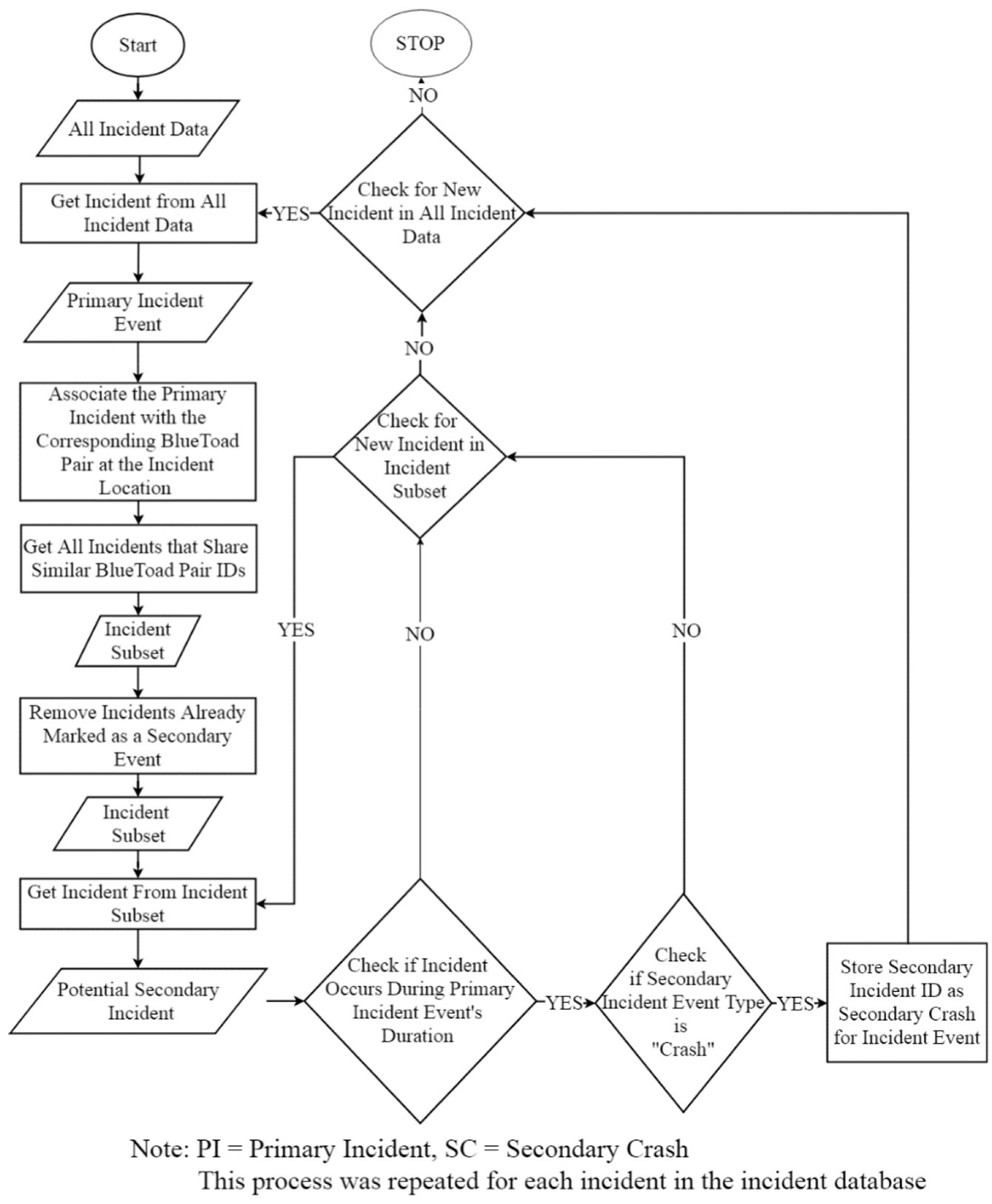
Before identifying SCs using the static method, ArcGIS, a mainstream Geographical Information System software, was used to assign mileposts (from Interstate shapefile) to all incidents. Next, the process of detecting SCs using the static method was automated by implementing an algorithm (Figure 2) in the Visual Basic for Applications (VBA) programming language. As mentioned earlier, SCs can occur either in the upstream direction of the PI or in the opposite direction of the PI. Although the primary event could be any incident and not necessarily a crash, this method focuses on identifying only SCs (and not secondary incidents). Thus, as one of the initial steps, the potential secondary incidents are checked to make sure they are in fact crashes (Figure 2).

Figure 2.

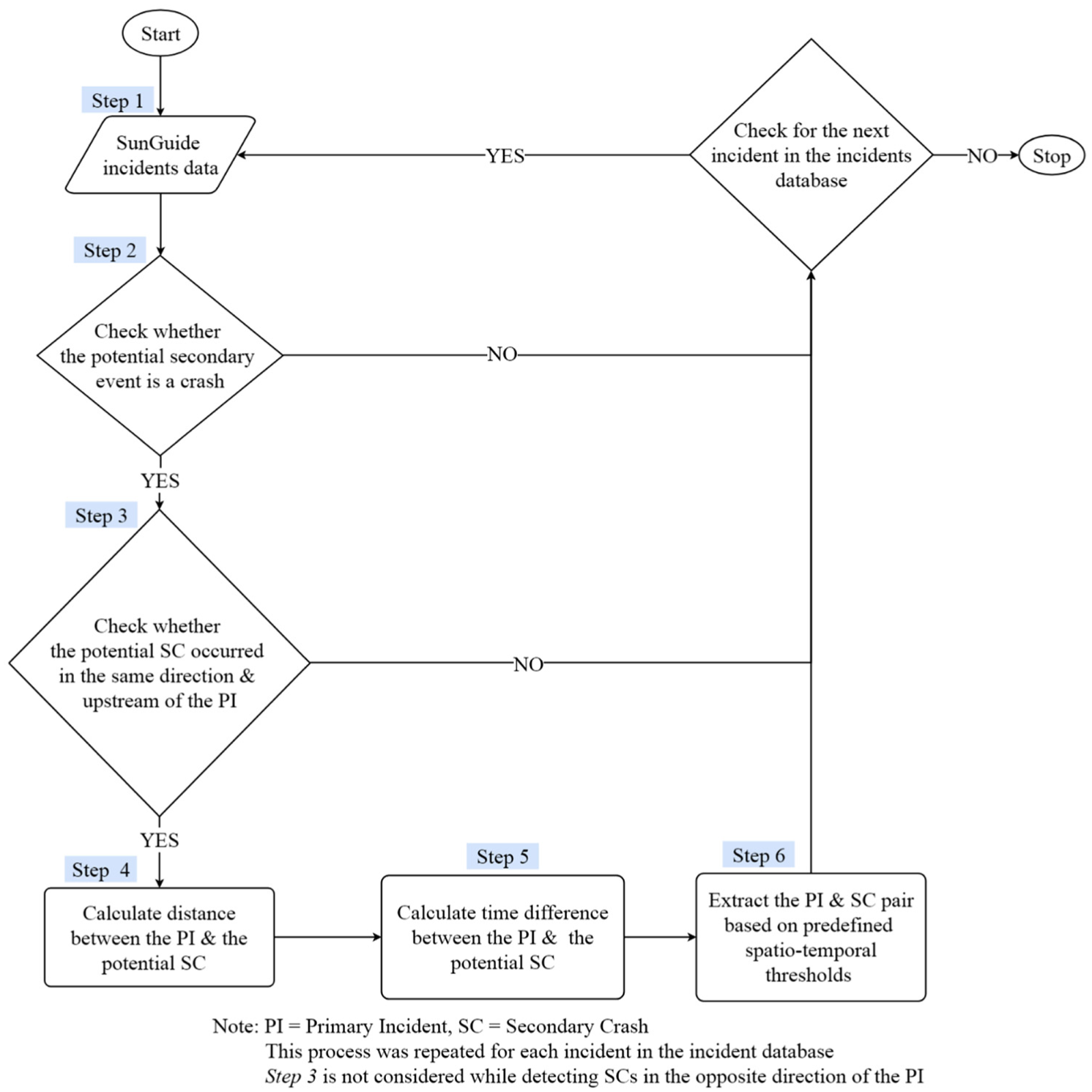
Algorithm to identify SCs using the static method.

The occurrence of a PI is expected to result in a queue backup in the upstream direction (and not in the downstream direction). Therefore, SCs that occurred only in the direction and upstream of the PI are identified by comparing the milepost of the PI with the milepost of the potential SCs. The mileposts of the PI and the potential SCs are used to compute the distance between the two incidents. The time difference between the PI and the potential SC is calculated. Following the identification of the spatiotemporal relationship between the PI and the potential SC, the respective pairs are extracted based on the set spatiotemporal criteria. The extracted SCs are stored, and the process is repeated for the rest of the incidents in the SunGuide^™ database. It is worth noting that one PI can result in more than one SC.

To identify SCs in the opposite direction of the PI, half a mile was used as the spatial threshold and incident clearance duration of the PI was used as the temporal threshold. All the steps in Figure 2 except Step 3 were used to detect SCs in the opposite direction of the PI. Note that SCs in the opposite direction can occur both on the upstream and downstream of the PI.

Dynamic Method Algorithm

The proposed dynamic approach focuses on identifying the impact range of the PI using speed data collected by the BlueToad^® paired devices and detecting SCs occurring within the spatiotemporal impact range of the PI. This method aims to better capture the effects of traffic flow characteristics, such as speed, that change over space and time and affect the queue formation as a result of a PI.

Incident Impact Duration Estimation

Before computing the impact range of the PI, the raw speed data from BlueToad^® paired devices were aggregated in 15-min intervals and extracted to determine the spatiotemporal effects of PIs under the prevailing traffic conditions. Note that natural traffic flow data at shorter time intervals normally contain a large amount of noise ( 24 ), and previous literature has recommended using a minimum of 15-min measurement intervals to obtain stable traffic flow rates ( 25 ).

Each incident was first matched to a specific BlueToad^® pair located along the roadway segment based on geographic coordinates. The speed data at the time of each incident were retrieved from the matched BlueToad^® pair. Historical speed data for the BlueToad^® device pairs with matched incidents were used to establish recurrent speed profile of the section under normal traffic conditions. In addition, a confidence interval of one standard deviation was established to define the upper and lower bounds of the speed profile (i.e., speed bandwidth) to account for recurrent speed variations.

Figure 3 provides an example of how the incident impact duration is estimated from speed profiles. The blue dotted line in the figure shows the average 15-min speeds for a 24-h period at a specific location. The orange continuous lines show the confidence interval of one standard deviation. These bounds help take into consideration the speed variations in recurrent conditions. In the example depicted in Figure 3, an incident was recorded at 4:30 p.m., and the blue solid line shows the speeds at this location after the incident occurred. As can be observed from Figure 3, the speeds returned to normal condition at around 7:30 p.m., and the impact duration of this incident is estimated to be about 3 h.

Figure 3.

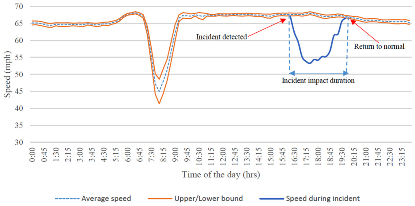
Estimation of incident impact duration from speed profiles.

The incident impact duration was computed for incidents that were successfully matched to the BlueToad^® devices. This process was achieved by tracking the BlueToad^® reported speeds at the segment of the incident occurrence from the time of the incident detection to the time when the traffic flow returned to normal. As can be inferred from Figure 3, the time it takes from incident detection to the return to normal speeds is recorded as the incident impact duration. A similar procedure is repeated for all incidents in the dataset.

Identification of SCs

Following the establishment of the recurrent speed for each of the incident-related BlueToad^® device pair, aggregated 15 min speed data from the time of the incident occurrence were collected to identify upstream BlueToad^® pairs affected by the incident. Figure 4 provides the framework of the algorithm used to identify SCs using speed data.

Figure 4.

Identification of SCs using speed data.

For each of the incident subset, the retrieved vehicle speeds from the incident reported time were compared with the recurrent speeds of the respective pairs. The incident subset in Figure 4 refers to a set of incidents that occurred within a similar BlueToad^® pair device. A BlueToad^® pair is considered to be affected by the occurrence of an incident when the speeds from the incident reporting times are lower than the defined boundary of recurrent speeds.

Once all the BlueToad^® pairs affected by the incident subset are identified, the BlueToad^® pairs are then checked to identify whether there was another incident occurring within the affected BlueToad^® pairs. All incidents identified within the affected BlueToad^® pairs are checked to determine whether they occurred within the time that the current speed falls below the average speed of the respective BlueToad^® pair. Next, from all incidents identified in the incident duration of the prior incident, only crashes are retrieved and considered as SCs. A crash is identified as “secondary” if it occurred within the impact area of a PI. This applied for crashes occurring both on the upstream and opposite direction of the PI.

Figure 5 describes the example of incidents that occurred on Monday, August 29th, 2016, along I-95 NB in 15-min speed intervals. On this particular day, 10 incidents that occurred along the study corridor resulted in significant congestion, that is, average speeds dropped below the recurring speeds along this corridor. Three of these 10 incidents were identified as SCs.

Figure 5.

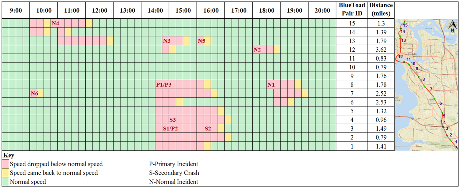
Detection of secondary crashes using BlueToad® speed data ( 26 ).

An incident occurred at 2:51 p.m. and affected eight BlueToad® pairs on the upstream direction (8.5 mi). It is worth noting that the speed along the BlueToad® pair #6 came back to normal much earlier than the rest of the pairs. As a result of congestion caused by the primary incident (P1), drivers might have detoured to other parallel routes (e.g., I-295). BlueToad® pair #6 is the only pair with an exit in the middle of two Bluetooth devices. This incident (P1) resulted in a SC (S1) that occurred 16 min later and 7.8 mi upstream of P1. This SC, S1, resulted in a significant drop in speeds on the pair that it occurred (#5) plus two other pairs (#3 and #4) on its upstream direction. About 36 min later, the same PI (P1, also identified as P3) resulted in another SC (S3) at about 7.01 mi upstream of P1. This incident resulted in a significant non-recurring congestion on the pair that it occurred (#4) and three other pairs on the upstream direction (#1, #2, and #3).

Incident S1 turned out to be a tertiary crash, which means that it is a SC that became a PI (P2) to another SC (S2), representing cascading events. Incident P2, which occurred at 3:07 p.m. along BlueToad^® pair #3 affected one additional pair #2, on the upstream direction. Secondary crash S2 occurred on the same pair (#5) as its PI 85 min later and affected one pair in the upstream direction (#4). It can be inferred from this observation that apart from resulting in non-recurring congestion, SCs can also lead to additional crashes, here referred to as tertiary crashes. In general, several of the SCs were found to contribute to additional crashes. Six of the incidents in Figure 5 are normal incidents, meaning that they did not result in SCs. For example, the normal incident N1 occurred at 6:57 p.m. on pair #8 and resulted in a significant drop in speed along two additional pairs (#6 and #7) on the upstream direction.

Results and Discussion

SCs Identified using the Dynamic Method

This approach used traffic incident data (6,865) from the SunGuide^™ database and real-time speed data from the BlueToad^® pairs. Overall, 518 SCs were identified from 425 PIs. The identified SCs accounted for 8% of the 6,865 incidents used in the analysis. The 425 PIs that induced SCs were 7% of all normal incidents (6,865 – (518 + 425)) = 5,922). These results indicate that approximately one in every 11 normal incidents was associated with a SC. Each PI caused an average of 1.2 SCs. Out of 518 incidents that were identified as SCs, 47 crashes resulted in additional crashes (40 resulted in an additional SC, and seven resulted in multiple additional SCs). SCs that occurred in the upstream direction constituted 87% of the total SCs, and the remaining 13% occurred in the opposite direction.

Figure 6 shows the temporal and spatial characteristics of SCs in relation to the PIs. Temporally, approximately 87% of the SCs were found to occur within 2 h after the occurrence of PIs. Spatially, 73% of the SCs were found to occur within 2 mi from the PI. Generally, 66% of SCs occurred within 2 h of the onset of a PI and within 2 mi upstream of the PI. In other words, about 34% of SCs occurred beyond the most commonly used 2-mi 2-h spatiotemporal threshold. These statistics confirm that the proposed dynamic approach identified more SCs than the traditional static method (2-mi and 2-h), that is, the static method underestimated the SCs.

Figure 6.

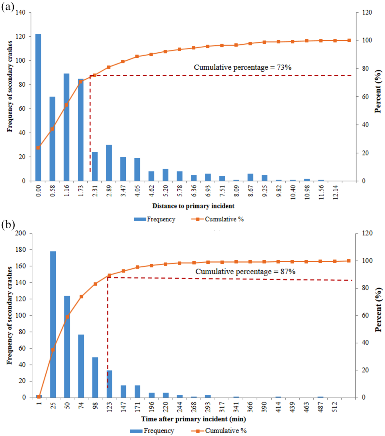
Spatiotemporal distribution of secondary crashes (SCs) in relation to primary incidents: (a) Spatial distribution and (b) Temporal distribution.

SCs Identified using the Static Method

SCs were also identified using the static method to evaluate the sensitivity of spatiotemporal thresholds and to determine the extent of under/overestimation of SCs when compared with the dynamic method. The spatiotemporal thresholds of 2.5 h and 5 mi were adopted to detect SCs on the upstream direction of the PI. This is because 90% of SCs detected by the dynamic method were found to occur within these thresholds. More specifically, 15-min temporal thresholds (i.e., 15, 30, … 150 min) were used along with the 0.5-mi spatial thresholds (i.e., 0.5, 1, …, 5 mi). Meanwhile, SCs on the opposite direction were identified based on 0.5-mi spatial threshold and PI clearance duration as the temporal threshold. Figure 7a gives the frequency of SCs identified using the static method. Based on the adopted spatiotemporal thresholds, 554 SCs were identified using the static method. As expected, the number of SCs increased with the increase in spatial and temporal thresholds. It can be inferred from Figure 7a that the static method begins to overestimate the SCs beyond the 4.5-mi and 150-min thresholds, when compared with the dynamic method that identified 518 SCs. Further, the rate of change of frequency of SCs is sparser within the 2.5-mi threshold and denser beyond the 2.5-mi threshold. Notably, the use of longer thresholds does not necessarily mean that all the detected SCs are accurately identified (i.e., there are no false positives). This scenario is further explained in Figure 7b in which the proportion of SCs identified by the static method and the dynamic method decreases with the increase in the spatiotemporal thresholds. In Figure 7b, SCs detected within 1 mi have an overall highest proportion of matched SCs (76%) compared with the rest of the spatial thresholds. Meanwhile, SCs detected using a 5-mi spatial threshold had the least proportion of matched SC frequencies (69%). Further, the proportion of SCs detected using a spatial threshold of 0.5 mi significantly dropped beyond 60 min.

Figure 7.

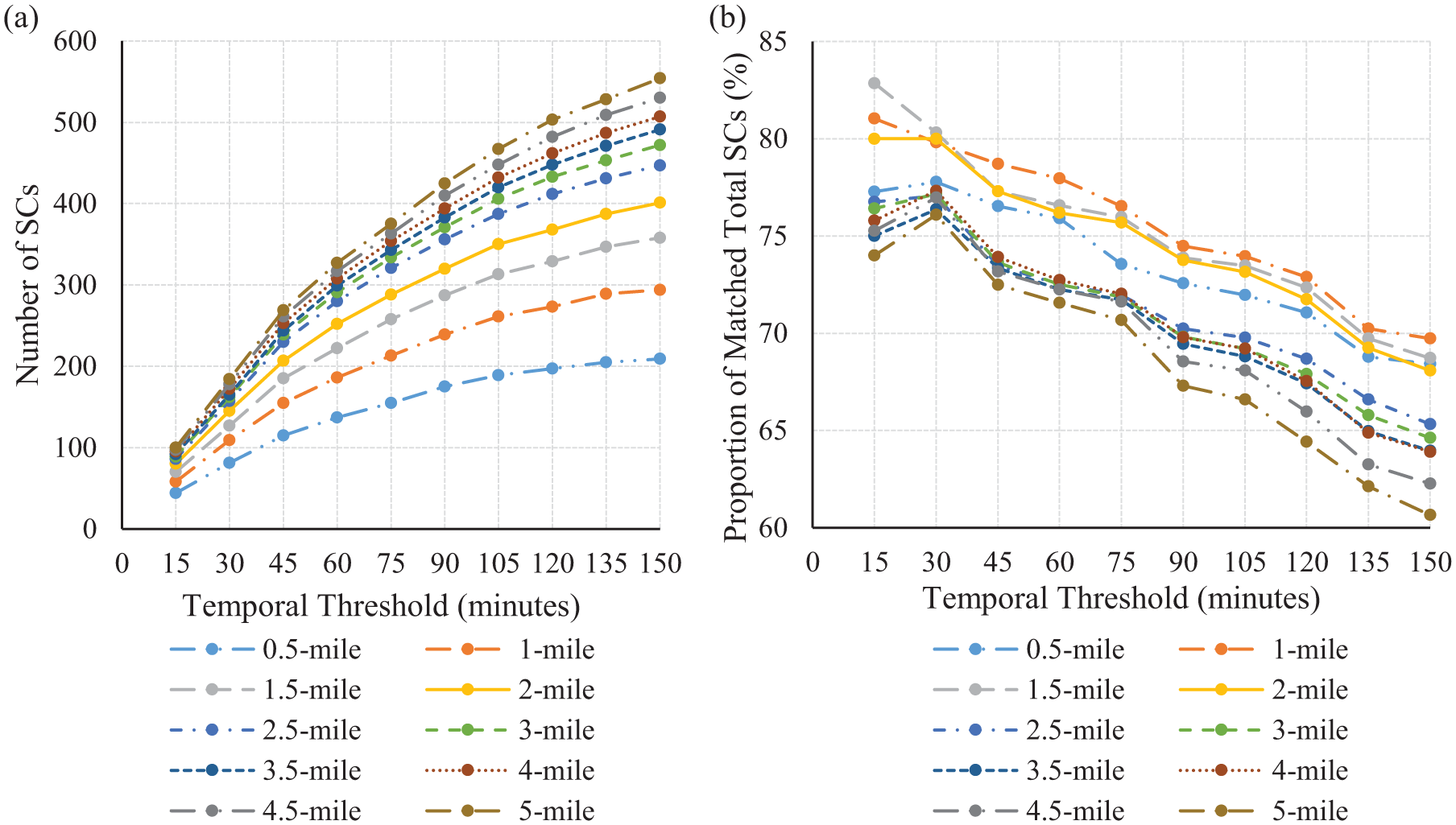
Secondary crashes (SCs) identified using the static method: (a) SCs identified using the static method and (b) Proportion of SCs identified using the static method that were matched with the SCs identified using dynamic method.

Impact of Prevailing Traffic Condition on SC Occurrence

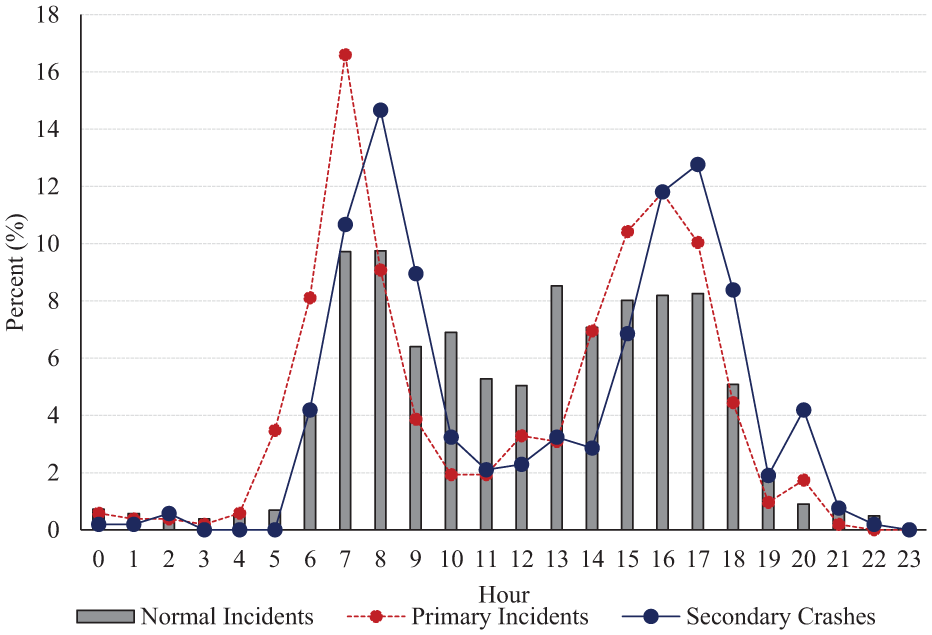
Figure 8 shows the distribution of the 518 SCs and 425 PIs identified using the dynamic method, and 6,347 normal incidents by different time periods. It can be deduced from the plot that only 1% of SCs occurred between midnight and 5:00 a.m. whereas 80% occurred during peak hours, that is, morning peak, 6:00–9:00 a.m. and evening peak, 3:00–6:00 p.m. Specifically, 38% of SCs occurred during morning peak, and the remaining 42% occurred during evening peak.

Figure 8.

Dynamic traffic incidents distribution by time of day.

The highest proportion of PIs (17%) was observed at 7:00 a.m., whereas the highest proportion of SCs (15%) occurred 1 h later, that is, at 8:00 a.m. The other peak times for the PIs (12%) and SCs (13%) were found to be at 4:00 p.m. and 5:00 p.m., respectively. The corresponding normal incidents were also at their highest during these particular hours, resulting in 60% of all normal incidents. In summary, more than three-quarter of detected SCs (78%) occurred during congested traffic condition (Table 2). This could be attributed to the fact that congested traffic is characterized with smaller gaps between vehicles, providing drivers with lesser maneuvering room to avoid a crash.

Table 2.

Impact of Prevailing Traffic Condition on Incident Occurrence

	Prevailing traffic condition
	Congested period		Uncongested period
Incident category	6:00–9:00	15:00–18:00	9:01–14:59	18:01–05:59
Normal incidents (%)	30	30	32	8
Primary incidents (%)	38	37	17	8
Secondary crashes (%)	38	40	14	8
Distance (mile)	1.4	1.7	1.5	2.6
Time (min)	50.7	51.3	64.5	84.0

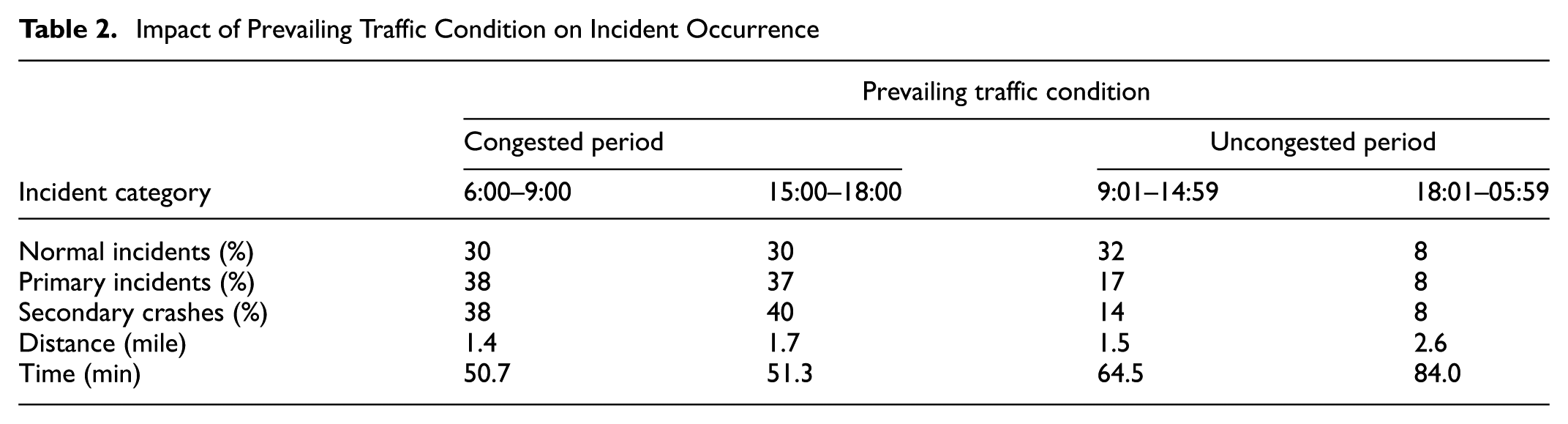
Figure 9 shows the impact areas for PIs that resulted in SCs within a threshold of 1 mi and 60 min. These impact areas refer to incidents that occurred when the prevailing traffic condition is under congested state and when it is under uncongested state. There is a significant dispersion with respect to the impact areas during congested and uncongested traffic flow conditions. It could be inferred from Figure 9 that prevailing traffic conditions is one of the major factors that influence the spatial and temporal locations of SCs. In other words, prevailing traffic flow characteristics were found to affect the manner in which the disturbance caused by the PI propagates in the upstream direction.

Figure 9.

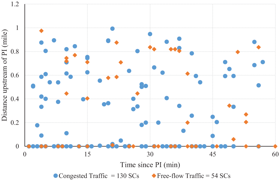
Spatiotemporal extent of secondary crashes (SCs) from their respective primary incidents (PIs).

Considering the influence of prevailing traffic conditions on the occurrence of SCs, the number of SCs identified using the static method were also compared with the number of SCs identified using the dynamic method based on traffic flow characteristics, that is, during uncongested (off-peak hours) and congested (peak hours) conditions. Figure 10a and b show the proportion of SCs identified by both the static and dynamic methods during congested and uncongested conditions, respectively. There is a clear demarcation between the proportion of matched SCs that occurred within 2 mi and beyond 2 mi during congested traffic conditions. Compared with uncongested traffic conditions, there is a higher match of SCs occurring on congested traffic within 0.5 mi from the PI. Whereas the greatest match of SCs on congested traffic is within 1 mi (83%), the greatest match during uncongested traffic conditions is within 2 mi (78%). These results indicate that there is a distinct difference in the PI impact area under uncongested and congested traffic conditions. Therefore, using fixed spatiotemporal thresholds to detect SCs during congested and uncongested conditions could lead to inaccurate results.

Figure 10.

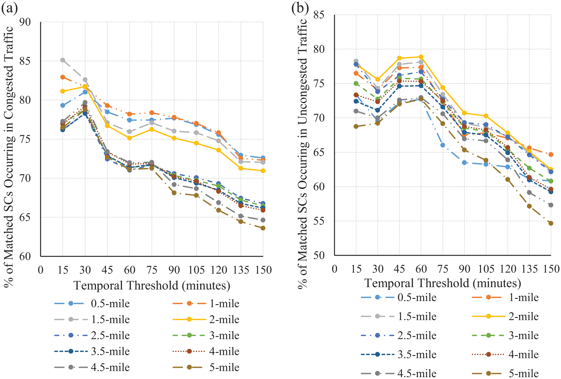
Proportion of secondary crashes (SCs) identified using the static method that were matched with the SCs identified using dynamic method in congested and uncongested traffic conditions: (a) In congested traffic and (b) In uncongested traffic.

Summary and Conclusions

FHWA has established the reduction of SCs as one of the performance measures for incident management programs. As such, proper identification of SCs is pivotal to accurate reporting of the effectiveness of the programs deployed to mitigate SCs. Nevertheless, the detection of SCs is not a straightforward procedure as the definition itself is subjective, a situation that largely impeded strategies for their mitigation. Past studies have proposed static and dynamic approaches to identify SCs; however, both of the approaches have serious limitations that affect their practical applications. Although the dynamic method is proven to yield accurate and reliable results, applying it requires real-time traffic data which are only available on limited locations. On the other hand, whereas the static method is still the most viable approach for practical applications, its one-size-fits-all approach of using fixed spatiotemporal thresholds does not yield reliable results. This is because the impact area of the PI heavily depends on the prevailing traffic conditions, that is, uncongested or congested conditions. This study focused on investigating the impact of PI spatiotemporal influence thresholds on the detection of SCs. More specifically, the impact of spatiotemporal thresholds on uncongested and congested traffic states and the sensitivity of varying spatial and temporal limits of PIs on the detection of SCs were investigated.

The present study identified SCs on freeways using both the static and dynamic methods along I-95, I-10, and I-295 corridors in Jacksonville, Florida. For the dynamic method, this study focused on identifying the impact range of the PI using prevailing speed data extracted from the BlueToad^® pairs. This method aims to better capture the effects of traffic flow characteristics, such as speed that changes over space and time and affects the queue formation as a result of a PI. Overall, 518 SCs were identified from 425 PIs. The identified SCs account for 8% of the 6,865 incidents used in the analysis. The study also developed a VBA script to statically identify SCs based on conventionally adopted spatiotemporal thresholds. To facilitate the comparison of the SC frequencies detected using the dynamic and static methods, the spatial threshold of 5 mi and temporal threshold of 150 min were adopted. This is because 90% of SCs detected using the dynamic method occurred within these thresholds. The predefined spatiotemporal thresholds were further divided into 15 min temporal thresholds (i.e., 15, 30, … 150 min) along with the 0.5-mi spatial thresholds (i.e., 0.5, 1, …, 5 mi). On the other hand, SCs on the opposite direction were identified based on 0.5-mi spatial threshold and PI clearance duration as the temporal threshold.

The study results indicated that 78% of SCs occurred during peak hours, that is, morning peak, 6:00–9:00 a.m. and evening peak, 3:00–6:00 p.m. The highest proportion of PIs (17%) occurred at 7:00 a.m., while the highest proportion of SCs (15%) occurred 1 h after the PI, that is, at 8:00 a.m. Comparison of SC frequencies identified using the static and dynamic methods showed that the static method consistently under and overestimated SC frequencies for smaller and larger spatiotemporal thresholds, respectively. This phenomenon is expected, as most SCs have a high probability of occurrence within the 15–60 min and 0.5–1 mi spatiotemporal thresholds, and a low probability of occurrence within 150-min and 5-mi spatiotemporal thresholds. It was observed that prevailing traffic conditions play a crucial role in instigating SCs; more than three-quarters of SCs occurred during congested traffic conditions.

In practice, the proposed dynamic method can be easily implemented. Its identification algorithm does not need much computational effort. The only part that requires substantial computational effort is developing the historical non-incident speed profiles, which need to be computed only once and can be used for a prolonged period of time—months and potentially up to a year. The proposed method can be used by incident management agencies to automate production of regular reports on a monthly, quarterly, and yearly basis. Also, with additional programming work, the proposed method can be used to detect SCs in real time. Use of the derived spatiotemporal thresholds is expected to reduce the biases associated with the subjective thresholds used by the static method. Further, the study results could be used to develop several active traffic management strategies such as dynamic lane use control to mitigate SCs. Connected and automated vehicle technology, once adopted, could not only mitigate SCs but also improve the overall safety and mobility of freeways.

Limitations and Future Work

This study used speed data from BlueToad^® devices, and incident data from the SunGuide^™ database. Speed data extracted from the BlueToad^® devices were used to determine the spatiotemporal impact range of PIs, and thus to identify SCs. However, the BlueToad^® devices, with an average spacing of 1.7 mi, may not be able to precisely capture the speed changes over space. Although incidents were found to usually have longer spatial impacts in the upstream direction, affecting multiple BlueToad^® pairs, using speeds along shorter sections could potentially capture the realistic traffic dynamics, including queue formation and dissipation.

As BlueToad^® pairs become more prevalent and as crowdsourced travel speed data become more readily available, future studies can incorporate virtual detectors that use crowdsourced traffic information to obtain additional traffic speed data. Moreover, with the use of crowdsourced traffic data, the study locations do not have to be limited to the corridors with active BlueToad^® devices.

Footnotes

Acknowledgements

This research was sponsored by the Florida Department of Transportation (FDOT) and conducted as a cooperative effort by the Florida International University (FIU) and the University of North Florida (UNF).

Author Contributions

The authors confirm contribution to the paper as follows: study conception and design: AEK, PA, and TS; data collection: AEK and RL; analysis and interpretation of results: AEK, PA, and TS; draft manuscript preparation: AEK, PA, TS, and RL. All authors reviewed the results and approved the final version of the manuscript.

The Standing Committee on Safety Data, Analysis and Evaluation (ANB20) peer-reviewed this paper (19-02583).

The opinions, findings, and conclusions expressed in this publication are those of the authors and not necessarily those of the Florida Department of Transportation or the U.S. Department of Transportation.

References

Baykal-Gürsoy

Xiao

Ozbay

Modeling Traffic Flow Interrupted by Incidents. European Journal of Operational Research, Vol. 195, No. 1, 2009, pp. 127–138.

Owens

Amstrong

Sullivan

Mitchell

Newton

Brewster

Trego

Traffic Incident Management Handbook. Publication FHWA-HOP-10-013. FHWA, U.S. Department of Transportation, Washington, D.C., 2010.

Moore

J. E.

Giuliano

Cho

Secondary Accident Rates on Los Angeles Freeways. Journal of Transportation Engineers, Vol. 130, No. 3, 2004, pp. 280–285.

Zhang

Khattak

What is the Role of Multiple Secondary Incidents in Traffic Operations?

Journal of Transportation Engineering, Vol. 136, No. 11, 2010, pp. 986–997.

Yang

Bartin

Ozbay

Mining the Characteristics of Secondary Crashes on Highways. Journal of Transportation Engineering, Vol. 140, No. 4, 2014, p. 04013024.

Karlaftis

M. G.

Latoski

S. P.

Richards

N. J.

Sinha

K. C.

ITS Impacts on Safety and Traffic Management: An Investigation of Secondary Crash Causes. ITS Journal - Intelligent Transportation Systems Journal, Vol. 5, No. 1, 1999, pp. 39–52.

Yang

Ozbay

Xie

Assessing the Risk of Secondary Crashes on Highways. Journal of Safety Research, Vol. 49, 2014, pp. 143.e1–e149.

Vlahogianni

E. I.

Karlaftis

M. G.

Orfanou

F. P.

Modeling the Effects of Weather and Traffic on the Risk of Secondary Incidents. Journal of Intelligent Transportation Systems, Vol. 16, No. 3, 2012, pp. 109–117.

O’Laughlin

Smith

Operational issues discussion paper on incident management operations: Top five issues. Proc., National Conference on Traffic Incident Management: A Road Map to the Future, Irvine, CA, 2002, p. C-2.

10.

NCHRP. Guidance for Implementation of Traffic Incident Management Performance Measurement/ Performance Measurement for Traffic Incident Management Programs/Florida. http://nchrptimpm.timnetwork.org/?page_id=79. Accessed February 12, 2018.

11.

Lou

Yin

Lawphongpanich

Freeway Service Patrol Deployment Planning for Incident Management and Congestion Mitigation. Transportation Research Part C: Emerging Technologies, Vol. 19, No. 2, 2011, pp. 283–295.

12.

Yang

Wang

Xie

Ozbay

Imprialou

Methodological Evolution and Frontiers of Identifying, Modeling and Preventing Secondary Crashes on Highways. Accident Analysis and Prevention, Vol. 117, 2018, pp. 40–54.

13.

Chang

G. L.

Rochon

Performance Evaluation and Benefit Analysis for Chart-the Real-Time Incident Management System. Final Report. State Highway Administration of Maryland, Baltimore, MD, 2011.

14.

Kopitch

Saphores

J. D. M.

Assessing Effectiveness of Changeable Message Signs on Secondary Crashes. Presented at 90th Annual Meeting of the Transportation Research Board, Washington, D.C., 2011.

15.

Jalayer

Baratian-Ghorghi

Zhou

Identifying and Characterizing Secondary Crashes on the Alabama State Highway Systems. Advances in Transportation Studies, Vol. 37, 2015, pp. 129–140.

16.

Tian

Chen

Truong

A Case Study to Identify Secondary Crashes on Interstate Highways in Florida by Using Geographic Information Systems. Advances in Transportation Studies, Vol. 2, 2016, pp. 103–112.

17.

Vlahogianni

Karlaftis

Golias

Halkias

Freeway Operations, Spatiotemporal-Incident Characteristics, and Secondary-Crash Occurrence. Transportation Research Record: Journal of the Transportation Research Board, 2010. 2178: 1–9.

18.

Sun

C. C.

Chilukuri

The Use of Dynamic Incident Progression Curve for Classifying Secondary Accidents. Presented at 85th Annual Meeting of the Transportation Research Board, Washington, D.C., 2006.

19.

Yang

Ozbay

Morgul

Bartin

Xie

Development of Online Scalable Approach for Identifying Secondary Crashes. Transportation Research Record: Journal of the Transportation Research Board, 2014. 2470: 24–33.

20.

Goodall

N. J.

Probability of Secondary Crash Occurrence on Freeways with the Use of Private-Sector Speed Data. Transportation Research Record: Journal of the Transportation Research Board, 2017. 2635: 11–18.

21.

Park

Haghani

Real-Time Prediction of Secondary Incident Occurrences Using Vehicle Probe Data. Transportation Research Part C: Emerging Technologies, Vol. 70, 2016, pp. 69–85.

22.

Yang

Wang

Xie

Dai

Use of Ubiquitous Probe Vehicle Data for Identifying Secondary Crashes. Transportation Research Part C: Emerging Technologies, Vol. 82, 2017, pp. 138–160.

23.

Sarker

A. A.

Naimi

Mishra

Golias

M. M.

Freeze

P. B.

Development of a Secondary Crash Identification Algorithm and Occurrence Pattern Determination in Large Scale Multi-Facility Transportation Network. Transportation Research Part C: Emerging Technologies, Vol. 60, 2015, pp. 142–160.

24.

Guo

Liu

Huang

Wei

Cao

Short-Term Traffic Flow Prediction Using Fuzzy Information Granulation Approach under Different Time Intervals. IET Intelligent Transport Systems, Vol. 12, No. 2, 2018, pp. 143–150.

25.

Smith

Ulmer

J. M.

Freeway Traffic Flow Rate Measurement: Investigation into Impact of Measurement Time Interval. Journal of Transportation Engineering, Vol. 129, No. 3, 2003, pp. 223–229.

26.

Kitali

A. E.

Alluri

Sando

Haule

Kidando

Lentz

Likelihood Estimation of Secondary Crashes Using Bayesian Complementary Log-Log Model. Accident Analysis and Prevention, Vol. 119, 2018, pp. 58–67.

Impact of Primary Incident Spatiotemporal Influence Thresholds on the Detection of Secondary Crashes

Abstract

Existing Methods for Identification of Secondary Crashes

Study Objective

Data

SunGuide™

BlueToad® Devices

Methodology

Static Method Algorithm

Dynamic Method Algorithm

Incident Impact Duration Estimation

Identification of SCs

Results and Discussion

SCs Identified using the Dynamic Method

SCs Identified using the Static Method

Impact of Prevailing Traffic Condition on SC Occurrence

Summary and Conclusions

Limitations and Future Work

Footnotes

Acknowledgements

Author Contributions

References

SunGuide^™

BlueToad^® Devices