Comparative Analysis of Empirical Bayes and Bayesian Hierarchical Models in Hotspot Identification

Abstract

Hotspot identification is an important step in the highway safety management process. Errors in hotspot identification (HSID) may result in an inefficient use of limited resources for safety improvements. The empirical Bayesian (EB) HSID has been widely applied as an effective approach in identifying hotspots. However, there are some limitations with the EB approach. It assumes that the parameter estimates of the safety performance function (SPF) are correct without any uncertainty, and does not consider temporal instability in crashes, which has been reported in recent studies. The Bayesian hierarchical model is an emerging technique that addresses the limitations of the EB method. Thus, the objective of this study is to compare the performance of the standard EB method and the Bayesian hierarchical model in identifying hotspots. Three methods (crash rate, EB, and the Bayesian hierarchical model) were applied to identify risky intersections with different significance levels. Four evaluation tests (site consistency, method consistency, total rank differences, and Poisson mean differences tests) were conducted to assess the performance of these three methods. The testing results suggest that: (1) the Bayesian hierarchical model outperforms the crash rate and the EB methods in most cases, and the Bayesian hierarchical model improves the accuracy of HSID significantly; and (2) hotspots identified with crash rates are generally unreliable. This is significant for roadway agencies and practitioners trying to accurately rank sites in the roadway network to effectively manage safety investments. Roadway agencies and practitioners are encouraged to consider the Bayesian hierarchical model in identifying hotspots.

The identification of crash hotspots (also known as prone sites, sites with promise, or black spots) is one of the most important tasks in the roadway safety management process. Errors in hotspot identification (HSID) can result in inefficient use of limited resources for safety improvements and cause additional loss of lives.

Various methods have been proposed for HSID ( 1 – 3 ), and researchers have been continuously improving the methods ( 4 – 8 ); unfortunately, sites identified by different methods and ranking criteria are not identical ( 9 ) (they are not discussed in detail here because of space limitations). Observed crash counts and crash rates were often used by roadway agencies, but analyses have shown that these two methods cannot account for the regression-to-the-mean (RTM) bias and are not reliable ( 10 , 11 ). Methods based on empirical Bayes (EB) have shown superiority in estimating safety as well as in identifying hotspots ( 8 , 10 ). The standard EB method combines the observed crash counts of one site and the predicted safety of similar sites. The latter is typically derived from a safety performance function (SPF). The EB method was included in the first edition of the Highway Safety Manual ( 12 ) and is widely used in HSID for its ability in correcting the RTM bias and increasing estimation precision. Although many studies have shown that the EB method always performs better than other common HSID methods, it is not without limitations. One critical issue with the EB method is the implementation of the SPF to predict crashes. The SPF is usually modeled using crash data occurring at a similar “reference” pool of sites. In the conventional EB method, the SPF assumes that the number of crashes at each site follows a Poisson distribution, and the number of crashes in each year is independent. In other words, there is no yearly variation in safety at each site when assuming that the traffic volume and other key roadway features remain at the same level. However, this is often not true. With the evolution in vehicles, driving behavior, roadway design standards, and so forth, crash data can be unstable over time ( 13 , 14 ). Without accounting for the instability of crashes, the HSID results estimated through the EB method may be inaccurate under certain situations. In addition, the EB method assumes that the parameters in a fitted SPF are the true estimates, which is also a problematic assumption, especially when the sample size of reference sites is low ( 15 – 17 ).

Recently, Fawcett et al. proposed a novel Bayesian hierarchical model (denoted as Bayesian hierarchical model hereafter) for estimating and predicting roadway safety ( 18 ). The main advantage of the Bayesian hierarchical model is incorporating crash counts from multiple time points, with the counts in more recent years lending more weight to safety estimates than the counts from time points further in the past. The proposed model is able to capture the temporal trend of crashes at a site. A previous study has discussed the structure of the Bayesian hierarchical model and its application to real crash data. It was also noted that the standard EB method is a special case of the Bayesian hierarchical model ( 18 ). However, the HSID results have not been examined to compare the two methods. It is unknown whether or not the novel Bayesian hierarchical model outperforms the commonly used EB method in HSID. As a result, the primary purpose of this paper is to comparatively analyze the performance of the EB method and the Bayesian hierarchical model in HSID. To achieve the objective, this study identifies hotspots of intersections using the two methods, separately. Evaluation tests are conducted to assess the performance of each method.

Methodology

The following two sections introduce the EB method and Bayesian hierarchical model for identifying hotspots, separately. For comparison purposes, the crash rate-based HSID method is also discussed in the first section.

Crash Rate- and EB-Based HSID Methods

As the name implies, the crash rate-based method mainly calculates the rate of crashes at each site, and ranks the sites by their rates. It is usually calculated by dividing the observed crash number by exposure (e.g., vehicle miles of traveling, or VMT). There are a few types of crash rates: target crash rates (considering target collisions only), equivalent crash rate (converting crashes into the same severity level by different weight), and so forth. For the purpose of this study, the total number of crashes and the exposure, as traffic volume traveling through an intersection, are considered (see the “Data Description” section for more details). Thus, the crash rate for a site is calculated as

Crash Rat e_{i, j} = \frac{Y_{i, j}}{Volum e_{i, j} \times N} \times 10^{5}

(1)

where

$Crash Rat e_{i, j}$ = crash rate at site i in period j (per $10^{5}$ vehicles per year);

$Y_{i, j}$ = total number of observed crashes at site i in period j;

N = number of years in period j; and

$Volum e_{i, j}$ = traffic volume at site i in period j.

Because the crash rate simply relies on the observed number of crashes and exposure at the sites, the randomness of crashes and RTM bias are not well addressed. It has been pointed out that the HSID results using crash rates are not reliable ( 10 , 19 , 20 ). Safety researchers proposed using an EB approach to correct for the RTM bias ( 21 – 23 ). With the EB approach, an estimate of the long-term safety of an entity is obtained from two sources, as described above. Let K be the observed number of crashes, which is Poisson-distributed, and let k be the expected crash count; the EB estimator of k is given as

\hat{k} = w \times E (k) + (1 - w) \times K

(2)

$\hat{k}$ denotes the EB estimate of the expected number of crashes. E(k) can be estimated by the crash prediction model. Many statistical models have been proposed by transportation safety analysts to predict safety ( 24 , 25 )—for instance, the negative binomial (NB) ( 26 ), the Poisson-lognormal ( 27 , 28 ), the Conway–Maxwell–Poisson ( 29 , 30 ), the gamma ( 31 ), the Sichel ( 11 , 24 ), the negative binomial-Lindley ( 32 ) models, and others ( 33 , 34 ). Among these models, the NB model has been the most frequently used for predicting crashes. The NB model has the following structure: the number of crashes y during a given time period is assumed to be Poisson-distributed, the probability mass function (PMF) for which is given by

p (y | λ) = \frac{λ^{y} \times \exp (- λ)}{y!}, λ > 0, y = 0, 1, 2, \dots,

(3)

where $λ$ = mean response of the observed crash counts during a given period.

The rate parameter $λ$ is assumed to be gamma distributed with $E (λ) = μ$ and $Var (λ) = μ^{2} \times σ^{2}$ . Equation 4 shows the probability density function (PDF) for $λ$ ( 35 ):

f (λ | μ, σ) = \frac{1}{{(μ \times σ^{2})}^{(1 / σ^{2})}} \times \frac{λ^{1 / σ^{2} - 1} \times \exp (- λ / μ σ^{2})}{Γ (1 / σ^{2})}

(4)

The NB distribution can be viewed as a mixture of Poisson distributions where the Poisson rate $λ$ is gamma distributed. The PDF of the NB (Equation 5) can be obtained by summing out $λ$ in Equation 4 [readers are referred to Hilbe ( 36 ) for complete derivation of the NB model]:

p (y | μ, σ) = \int_{0}^{\infty} \frac{λ^{y} \times \exp (- λ)}{y!} \frac{1}{{(μ \times σ^{2})}^{(1 / σ^{2})}} \times \frac{λ^{1 / σ^{2} - 1} \times \exp (- λ / μ σ^{2})}{Γ (1 / σ^{2})} d λ

(5)

p (y | μ, σ) = \frac{Γ (y + \frac{1}{α})}{Γ (y + 1) \times Γ (\frac{1}{α})} \times {(\frac{α \times μ}{1 + α \times μ})}^{y} \times {(\frac{1}{1 + α \times μ})}^{1 / α}

(6)

where

y = response variable;

$μ$ = mean response of the observation; and

$α = σ^{2}$ is the dispersion parameter.

With the NB model structure, the weight factor w in the EB method is given as ( 22 ):

w = \frac{1}{1 + α \times E (k)}

(7)

For the detailed procedures of estimating roadway safety and ranking sites using the EB method, readers are referred to ( 21 , 22 , 37 ).

Bayesian Hierarchical Model

Rather than estimating from a single before period, the Bayesian hierarchical model proposed by Fawcett et al. ( 18 ) incorporates counts from multiple past periods. This adjusts the variations over the past crash counts by an SPF [note that the researchers used an accident prediction model (APM), and it is essentially the same as a SPF]. For evaluating the model, a discrete time indicator $t$ is chosen from previous years and the current year, that is, $t < 0$ and $t = 0$ , respectively.

The SPF is used to overcome the effects of global trend and RTM, and it is assumed that

y_{j} (t) | λ_{j} (t) ~ {\begin{matrix} Poisson (λ_{j} (t)), t ⩾ 0 \\ NB (r = \frac{λ_{j} (t)}{c (t) - 1}, p = \frac{1}{c (t)}), t < 0 \end{matrix}

(8)

where $λ_{j} (t) = a_{j} μ_{j} (t) \exp (b_{j} t)$ with $a_{j} \in R_{> 0}, b_{j} \in R$ and $μ_{j} (t)$ estimated from a global SPF for all $t$ ; $c (t) = \exp (- t τ)$ with $τ \in R_{> 0}$ for $t < 0$ . A log-linear SPF is chosen to estimate $μ_{j} (t)$ with an assumed NB over-dispersion parameter $γ$ as in

μ_{j} (t) = \exp (β_{0} + β_{t} t + \sum_{i = 1}^{M} β_{i} \log (n_{ij}) + \sum_{i = 1}^{N} β_{i} x_{ij})

(9)

Here, $n_{ij}$ and $x_{ij}$ indicate covariate information related to traffic volumes for $M$ such covariates and other observations for $N$ counts at each site $j$ . For prior distributions, Fawcett et al. ( 18 ) suggested using $a_{j} ~ Γ (γ, γ)$ , $b_{j} = b_{N} b_{z}$ with $b_{N} ~ N (μ_{N}, σ_{N}^{2})$ and $b_{Z} ~ Bernoulli (p_{B})$ , $τ ~ Γ (2, 20)$ after extensive prior trials. For $b_{N}$ and $b_{Z}$ , it is assumed that $μ_{N}$ follows a gamma distribution, $σ_{N}$ follows a normal distribution, and $p_{B}$ is beta-distributed. The regression coefficients in the SPF are given uninformative priors, so the model is relatively data-driven. Then, a Markov chain Monte Carlo (MCMC) procedure is employed to simulate the mean crash rates $λ_{j} (t)$ in the Bayesian framework, by making inferences on $a_{j}, b_{j}, τ_{j}$ with given prior specifications described above. With this structure, the Bayesian hierarchical model allows more recent observations to inform predictions with more certainty than observations further in the past. The choice of prior distribution for b_j ensures that local site-specific trends can be accounted for, over and above the global trend which is identified across the network, if this local trend at the site level is deemed significant.

Evaluation Methods

The crash rate method, the EB method, and the Bayesian hierarchical model are all techniques to identify hotspots. Evaluation tests on their performance are needed as rules to measure their performances in HSID. In most previous studies related to HSID, the percentage of false positives (FP) and percentage of false negatives (FN) have been the only measures. FP is the percentage of safe sites claimed to be unsafe, whereas FN occurs when an unsafe site has failed to be identified. Because the feedback from FP and FN is in binary format, this does not provide insight into the relative performance of HSID methods. For this study, four evaluation tests are implemented, namely: (1) the site consistency test; (2) the method consistency test; (3) the total rank differences test; and (4) the Poisson mean differences test. These tests not only include the consideration of FP and FN, but also take site ranking into account for evaluating the HSID method. These tests follow and reference the evaluation tests proposed by Cheng and Washington ( 19 ).

The site consistency test is to evaluate the ability of HSID methods by measuring the consistent appearance of a high-risk site over a subsequent observation period. The high-risk section includes sites $S_{j}$ with estimated crash rates or means from ${\hat{y}}_{(n - n α)}$ to ${\hat{y}}_{(n)}$ , ranking from $(n - n α)$ to $α$ at period $i$ , where $α$ is the significant level of the high risk. Test 1 compares the summation of crash rates for those identified high-risk sites at a later period $i + d$ after $d$ amount of observation time within all methods $m$ . Method A is better than other methods, when $T 1_{A, i + d} > \forall T 1_{\neq A, i + d}$ . The mathematical equation of this site consistency test when $T 2_{A} > \forall T 2_{\neq A}$ is

T 1_{\forall m, i + d} = \sum_{k = 1}^{k = n α} {\hat{y}}_{k, i + d}, j \in {j_{1} | {\hat{y}}_{(n - n α), i}, j_{2} | {\hat{y}}_{(n - n α + 1), i}, \dots, j_{(n - n α)} | {\hat{y}}_{n, i}}; d \in Z_{> 0}

(10)

The site consistency test evaluates the better method, with a higher output indicating a particular method is consistently good over sites.

The method consistency test looks at the consistency of the method over time periods, rather than being site based. For each method $m$ from $i$ to $i + d$ has its high-risk site range from ${S_{(n - n α)}, S_{(n - n α + 1)}, \dots, S_{(n)}}$ , that may or may not intersect with other HSID methods. This evaluation counts the numbers of elements in the intersection set, that is, it is counting the same sites that were identified as high risk formulated as

T 2_{\forall m} = | ⋂_{p = i}^{p = i + d} {S_{(n - n α)}, S_{(n - n α + 1)}, \dots, S_{(n)}}_{p} |; d \in Z_{> 0}

(11)

The method consistency test justifies a better method if a method scores higher than other methods, meaning such a method has larger numbers of similar high-risk sites identified throughout the time periods.

The third test, the total rank differences test, compares the summation of ranking differences between high-risk sites identified from base period $i$ to a later time period ( $i + d$ ). That is for every method $m$ , there are k sites identified as high-risk sites based on period $i$ . With these identified k sites, their corresponding rank $ℜ_{k, i + d}$ is found in period $i + d$ . The variations of the ranks are then summed as the output of this method as shown in

T 3_{\forall m} = \sum_{k = 1}^{k = n α} (ℜ_{k, i} - ℜ_{k, i + d}); k \in {S_{(n - n α)}, S_{(n - n α + 1)}, \dots, S_{(n)}}_{i}; d \in Z_{> 0}

(12)

Because it is a measure of variations of ranking, a smaller output indicates a better performance, that is $T 3_{A} < \forall T 3_{\neq A}$ .

Last, the Poisson mean differences test is used as an evaluation test in this study. It is an extension of the widely used false identification (FI) test. The FI test determines FN and FP as they appear in each HSID method. A site is justified as FN if it is truly hazardous, but mistakenly identified by a method as safe. On the other hand, if a site is truly safe but wrongly assessed as hazardous, it is then considered as FP. Therefore, it is important to have a knowledge of the truly hazardous sites and truly safe sites over time and space. However, the observed crash rate is site specific and time specific. The true Poisson mean (TPM) $\bar{y}$ is defined as the mean of the observed crash rates over the observation periods. The sites are then ranked based on the TPM as their true risk level, with a higher TPM assumed to be a truly riskier site. As sites are ranked by TPM, a critical TPM value is determined at a significance level $α$ in the rank. Such critical TPM, $TP M_{c}$ is the ruler in the Poisson mean differences test. Under the evaluation of this test, FNs and FPs of each method are identified with their corresponding TPM values, $TP M_{FN}$ and $TP M_{FP}$ . These then belong to the set $TP M_{FI} = TP M_{FN} \cup TP M_{FP}$ . Then, for each HSID method, the absolute differences between $TP M_{FI}$ and $TP M_{c}$ are summed over sites and time period. The test is mathematically formatted as

T 4_{\forall m} = \sum_{k = n - n α}^{k = n} \sum_{p = i}^{p = i + d} | TP M_{F I_{k, p}} - TP M_{C} |

(13)

The Poisson mean differences test is improved from the FI test by setting the associated TPM difference as the weight. In this test, a relatively small output for $T 4$ indicates less identification of false values in the HSID for a better performance in hotspot identification.

It is worth mentioning that researchers and practitioners have been using various measurements in ranking sites or network screening—for example, observed crash number or rate, EB method, difference between the EB and SPF (also known as potential for safety improvement, PSI), and ratio between the EB and SPF. Some previous studies ( 10 ) have shown that the EB method performs better than others in identifying hotspots. Thus, the EB method was utilized in this study.

Data Description

This study utilized the same data used by Fawcett et al. ( 18 ), but some filters were applied to exclude outliers and incomplete cases. The dataset includes annual accident counts from 2004 to 2012 at 734 intersections in the city of Halle, Germany. There are two types of observations in the dataset: numerical and binary. The numerical observations $n_{ij}$ are average traffic volume, traffic volumes from major and minor streets. The infrastructure observations $x_{ij}$ are represented in binary format, such as signalized or nonsignalized intersection, major or nonmajor intersection, and so on. Several adjustments are assigned to the original dataset. In safety analysis, if the traffic volume at a site is relatively low, collisions are rare and the TPM is small, making the parameter estimate unstable ( 17 ). In addition, sites with low traffic volume are less interesting to roadway agencies and practitioners. Therefore, thresholds are made for major and minor traffic volumes at 100 vehicles and 50 vehicles, respectively. That is, only the sites with a major volume of more than 100 vehicles and a minor volume of more than 50 vehicles are included in this study. In the meanwhile, considering that area type and traffic control have a significant effect on both operation and safety of intersections, this study focused on unsignalized intersections in urban areas only. This leaves 186 sites for this study. Table 1 provides summary statistics of the crash count and intersection features.

Table 1.

Summary Statistics of Accident Counts and Observations (186 Sites)

Variable	Min.	Max.	Mean (SD)
Crash (2004)	0	28	3.81 (4.30)
Crash (2005)	0	27	3.73 (4.34)
Crash (2006)	0	36	3.38 (4.42)
Crash (2007)	0	35	3.76 (4.55)
Crash (2008)	0	29	3.43 (4.09)
Crash (2009)	0	24	3.47 (4.10)
Crash (2010)	0	34	3.46 (4.29)
Crash (2011)	0	28	3.20 (4.27)
Crash (2012)	0	33	2.77 (3.83)
Average volume (vpd)	206	48,192	5,657.5 (7,168.1)
Major volume (vpd)	117	38,341	4,316.9 (5,447.2)
Minor volume (vpd)	52	23,498	1,340.6 (2,781.0)
Speed limit 30 km/h	Yes: 32.3%; No: 67.7%
Speed limit 45 km/h	Yes: 23.1%; No: 76.9%
Speed limit 50 km/h	Yes: 25.8%; No: 74.2%
Speed limit 60 km/h	Yes: 12.4%; No: 87.6%
Speed limit 70 km/h	Yes: 4.3%; No: 95.7%
Four legs	Yes: 23.1%; No: 76.9%

Note: min. = minimum; max. = maximum; SD = standard deviation; vpd = vehicles per day.

Results

Crash Rate and EB HSID

Crash rates over the 186 intersections for every 2 years were calculated using the definition documented in the previous section (i.e., Equation 1). A few examples are illustrated in Table 2. As can be seen, Site 74 ranked first in the period of 2004 and 2005, and the crash rate was 3,947.1 per 100,000 vehicles traveling per year. It varied from 1,879.7 to 2,255.6 in the following three periods. It ranked the sixth, tenth, and eighth in 2006 and 2007, 2008 and 2009, 2010 and 2011, respectively. Table 2 also lists the sites with relatively lower crash rates (see the bottom rows).

Table 2.

Example Sites of Crash Rate-Based HSID Results

	Year
Site no.	2004–2005	2006–2007	2008–2009	2010–2011
31	3,358.2 (2)^a	4,477.6 (1)	2,611.9 (3)	7,462.7 (1)
74	3,947.4 (1)	2,255.6 (6)	1,879.7 (10)	2,067.7 (8)
…	…	…	…	…
7	481.2 (47)	524.9 (39)	612.4 (39)	831.1 (34)
28	482.6 (46)	289.6 (69)	530.9 (44)	144.8 (92)
34	451.1 (49)	300.8 (64)	601.5 (40)	150.4 (91)
41	437.4 (50)	397.7 (54)	397.7 (54)	357.9 (60)
…	…	…	…	…
2	366.5 (63)	366.5 (56)	733.0 (36)	1,099.5 (27)
3	44.7 (146)	31.6 (147)	42.1 (140)	26.3 (146)
4	396.7 (58)	377.8 (55)	245.6 (74)	188.9 (81)
5	390.0 (61)	229.4 (79)	344.1 (63)	390.0 (57)

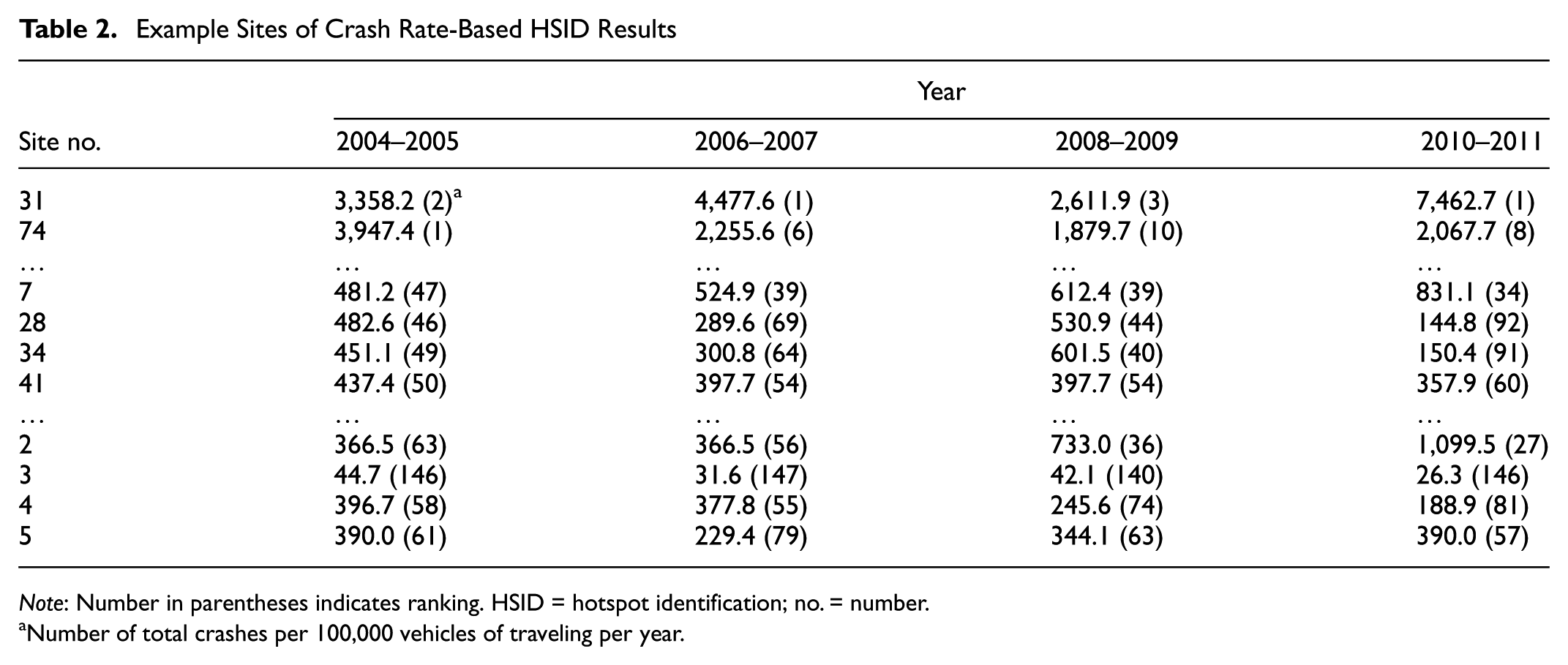
Note: Number in parentheses indicates ranking. HSID = hotspot identification; no. = number.

Number of total crashes per 100,000 vehicles of traveling per year.

As has been discussed, the SPF is an important part of the EB method. This study modeled the data with an NB distribution, and the modeling results are shown in Table 3. It is worth mentioning that an attempt was made to include all the variables in the model, because the main purpose of the SPF is prediction rather than inference. A few variables (e.g., speed limit 50, logarithm of major volume) are not significant at the 5% significance level, but they have been kept in the model. It is possible that some variables, such as volume and minor volume, are correlated, making the parameter estimates relatively unstable. However, this does not affect the prediction, which is of more interest in the EB method.

Table 3.

SPF of the NB Model

Variable	Estimate	SE	z value	Pr(>\|z\|)	Significance
Intercept	−1.0648	0.3471	−3.0678	0.0022	99%
Speed limit 30 km/h	0.9964	0.2120	4.7000	<0.0001	99%
Speed limit 45 km/h	0.6991	0.2308	3.0286	0.0025	99%
Speed limit 50 km/h	0.3780	0.0860	4.3979	<0.0001	99%
Speed limit 60 km/h	0.5022	0.0605	8.3036	<0.0001	99%
Speed limit 70 km/h	0.4715	0.2082	2.2647	0.0235	95%
Major intersection	0.1773	0.0520	3.4124	0.0006	99%
Four legs	−0.4696	0.2528	−1.8578	0.0632	na^a
Log (major volume)	1.3405	0.0704	na	na	95%
Log (minor volume)	−1.0648	0.3471	−3.0678	0.0022	99%
Log (volume)	1.0564	0.2242	4.7117	<0.0001	99%
Dispersion parameter	1.5314	0.2173	7.0458	<0.0001	99%
AIC	7,699.1

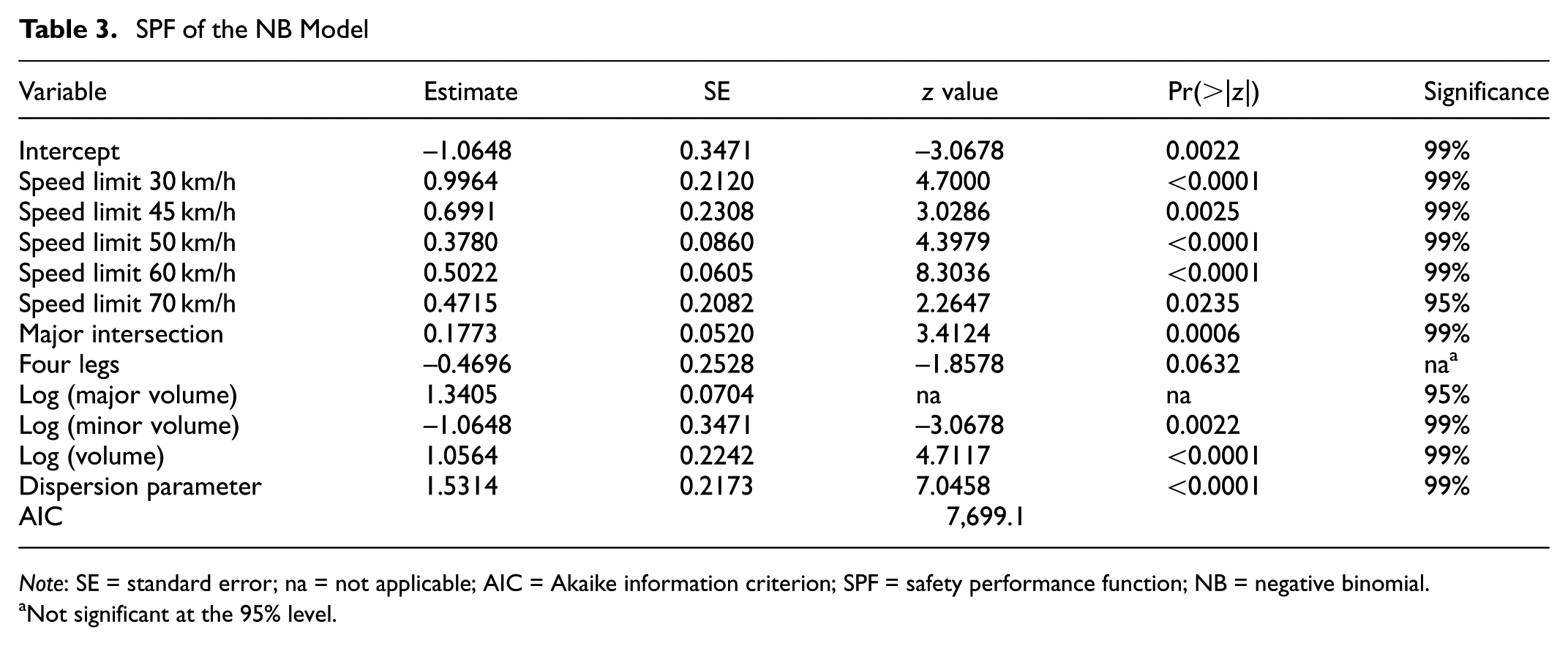
Note: SE = standard error; na = not applicable; AIC = Akaike information criterion; SPF = safety performance function; NB = negative binomial.

Not significant at the 95% level.

Using the SPF, the number of crashes for each site can be predicted, and the EB estimate is then calculated. Taking Site 9 as an example, the predicted number of crashes in 2004 is 8.39. The observed number of crashes in the year is 28. The weight is calculated as $w = \frac{1}{1 + 8.39 / 1.53} = 0.15$ . The EB estimate is $0.15 \times 8.39 + (1 - 0.15) \times 28 = 24.8$ . Similarly, the EB estimate at this site for 2005 is 23.2. The expected number of crashes in 2004 and 2005 together at this site is 48.0, shown in Table 4. Table 4 lists the expected number of crashes as well as rankings for selected sites.

Table 4.

Example Sites of EB-Based and Bayesian Hierarchical HSID Results

	Year
Site No.	2004–2005	2006–2007	2008–2009	2010–2011
EB-based method
9	48.0 (1)*	34.4 (3)	34.4 (4)	26.8 (4)
17	44.1 (2)	62.8 (1)	44.1 (1)	55.1 (1)
159	2.4 (164)	4.3 (108)	5.0 (97)	6.9 (56)
94	6.8 (73)	5.2 (91)	4.4 (106)	19.3 (9)
142	1.8 (180)	2.5 (154)	2.5 (154)	5.9 (74)
…	…	…	…	…
1	11.8 (28)	8.2 (53)	12.5 (22)	7.5 (48)
2	7.1 (69)	12.9 (21)	12.2 (25)	12.9 (19)
5	12.8 (26)	9.5 (42)	8.2 (48)	15.4 (15)
7	10.3 (37)	14.8 (16)	11.8 (28)	15.5 (14)
8	5.8 (87)	2.8 (148)	2.8 (148)	2.0 (171)
Bayesian hierarchical method
9	42.0 (4)^a	39.3 (4)	36.9 (4)	34.5 (4)
17	64.9 (1)	61.0 (1)	57.3 (1)	53.8 (1)
159	4.8 (105)	5.1 (95)	5.4 (83)	5.8 (74)
94	5.4 (96)	7.1 (69)	9.3 (42)	12.3 (21)
142	1.9 (161)	2.1 (153)	2.3 (144)	2.6 (130)
…	…	…	…	…
1	11.6 (40)	10.9 (38)	10.2 (38)	9.6 (39)
2	14.5 (21)	13.7 (20)	12.9 (20)	12.1 (22)
5	15.5 (16)	14.5 (15)	13.6 (15)	12.8 (17)
7	15.7 (15)	14.7 (14)	13.8 (14)	13.0 (16)
8	2.4 (148)	2.3 (149)	2.1 (151)	2.0 (150)

Note: Number in parentheses indicates ranking. no. = number; EB = empirical Bayesian; HSID = hotspot identification.

Expected number of crashes (in two years).

Bayesian Hierarchical Model

The Bayesian hierarchical model is coded in R for this study. The SPF model defined in Equation 9 estimates $μ_{j}$ with regression coefficients as well as dispersion parameter. The results are shown in Table 5. The covariates for urban area, intersection, signalization, major intersection, four leg intersection, and minor street traffic volume showed significant impact on the number of crashes. This is, overall, consistent with the NB model in EB method (please see Table 3). The estimated coefficient $β_{t}$ for year is negative, indicating that the number of crashes over the network displays a decreasing trend (without significant changes in other situations).

Table 5.

Regression Results of SPF in the Bayesian Hierarchical Model

Variable	Estimate	SE	z value	Pr(>\|z\|)	Significance
Intercept	−1.1926	0.3487	−3.4200	0.0006	99%
Speed limit 30 km/h	1.0658	0.2239	4.7595	<0.0001	99%
Speed limit 45 km/h	1.5398	0.2171	7.0933	<0.0001	99%
Speed limit 50 km/h	0.9092	0.2140	4.2489	<0.0001	99%
Speed limit 60 km/h	0.9974	0.2118	4.7102	<0.0001	99%
Speed limit 70 km/h	0.7091	0.2305	3.0762	0.0021	99%
Major intersection	0.3839	0.0857	4.4787	<0.0001	99%
Four legs	0.5083	0.0603	8.4314	<0.0001	99%
Log (major volume)	0.4754	0.2076	2.2900	0.0220	95%
Log (minor volume)	0.1766	0.0518	3.4065	0.0007	99%
Log (volume)	−0.4742	0.2521	−1.8809	0.0600	na^a
Year	−0.0316	0.0098	−3.2311	0.0012	99%
Dispersion parameter	1.3534	0.0714	na	na	99%
AIC	7,690.9

Note: SE = standard error; na = not applicable; AIC = Akaike information criterion; SPF = safety performance function.

Not significant at the 95% level.

Moreover, parameters are determined by their priors for MCMC methods. According to Fawcett et al. ( 18 ), the prior for the time-dependent inflation parameter $τ$ should be $τ ~ Γ (2, 20)$ . With the dispersion parameter obtained using maximum likelihood from the SPF, the prior of the site-specific crash modification factor $a_{j}$ is $a_{j} ~ Γ (1.3534, 1.3534)$ . The term $b_{j}$ , a prior weight to the local trend, is formed by $b_{N}$ and $b_{Z}$ , as explained in the “Methodology” section with $b_{N} ~ N (μ_{N}, σ_{N}^{2})$ and zero inflation $b_{Z} ~ Bernoulli (p_{B})$ . The study assumed $μ_{N} ~ N (0, 10), σ_{N} ~ Γ (0.1, 0.01)$ and $p_{B} ~ B (0.1, 0.1)$ , which are all weak informative priors. The MCMC procedure is then employed to simulate the mean crash rates $λ_{j} (t)$ in the Bayesian framework by making inferences on $a_{j}, b_{j}, τ_{j}$ with given prior specifications for a total $20, 000$ walks with 10 walks per step. Table 6 illustrates the parameters corresponding to sample Sites 9, 17, 41, and 67 with observed crash counts $y_{j}$ , SPF predicted crash rates $μ_{j}$ and the mean crash rate $λ_{j}$ in each pair of years. Table 6 shows MCMC results with local deviation adjuster $b_{j}$ , and discrepancy $a_{j}$ estimates the crash counts better than the SPF predictions. Here, for sites 9 and 17, the posterior means for b_js are very close to zero, that is, the trend of MCMC results for the site is almost parallel to SPF predicted crash rates. For sites 159 and 94, however, their b_js are relatively large, indicating the higher deviation in yearly crashes at the two intersections.

Table 6.

Observed Crash Count, SPF Prediction, and MCMC Results of Example Sites

				Year
Site No.	$a_{j}$	$b_{j}$	Crash	2004–2005	2006–2007	2008–2009	2010–2011
9	2.524 (2.091, 2.957)	–0.0008 (–0.016, 0.014)	$y_{j}$	54	38	38	29
	2.524 (2.091, 2.957)	–0.0008 (–0.016, 0.014)	$μ_{j}$	16.5	15.5	14.6	13.7
			$λ_{j}$	42.0	39.3	36.9	34.5
17	3.7544(3.245, 4.264)	0.0003(–0.009, 0.009)	$y_{j}$	49	71	49	62
	3.7544(3.245, 4.264)	0.0003(–0.009, 0.009)	$μ_{j}$	17.3	16.3	15.3	14.3
			$λ_{j}$	64.9	61.0	57.3	53.8
159	1.3794(0.174, 2.585)	0.0635(–0.155, 0.282)	$y_{j}$	1	4	5	8
	1.3794(0.174, 2.585)	0.0635(–0.155, 0.282)	$μ_{j}$	5.5	5.2	4.9	4.6
			$λ_{j}$	4.8	5.1	5.4	5.8
94	1.8098(0.538, 3.082)	0.1707(–0.074, 0.415)	$y_{j}$	6	4	3	22
	1.8098(0.538, 3.082)	0.1707(–0.074, 0.415)	$μ_{j}$	10.6	10.0	9.4	8.8
			$λ_{j}$	5.4	7.1	9.3	12.3

Note: SPF = safety performance function; MCMC = Markov chain Monte Carlo; no. = number; y = observed crash count; µ = SPF Prediction; λ = MCMC results.

Like the crash rate and EB results, Table 4 illustrates the example results for the Bayesian hierarchical method. Taking Site 9 as an example, the predicted number of crashes in 2004 and 2005 by SPF is 16.5. From MCMC, the associated $a_{j} = 2.524, b_{j} = - 0.0008$ are obtained. Then the Bayesian hierarchical estimate $λ_{j}$ is $16.5 \times 2.524 \times \exp (- 0.0008) \approx 42.0$ , shown in Table 4 and Table 6. The rank associated with each mean crash rate represents the ranking of the crash rate in the period. For example, Site 17 ranks highest in every pair, with an expected mean crash number of 64.9 for the period of 2004 and 2005, 61.0 for 2006 and 2007, 57.3 for 2008 and 2009, and 53.8 for 2010 and 2011. Site 17 ranks similarly, as first and second, with the EB-based method. However, not all sites rank similarly as Site 17 does. For example, Site 1 ranks 40th in 2004 and 2005 by the Bayesian hierarchical method, but ranks 28th in 2004 and 2005 by the EB-based method. It ranks 38th in 2006 and 2007 by the Bayesian hierarchical method, but ranks 53rd in 2006 and 2007 by the EB-based method. This leads to the evaluations of results as addressed in the next section to compare HSID methods.

Evaluation Results

As stated in the “Data Description” section, there are a total of 186 sites. With significance levels of 0.025, 0.050, and 0.075, there are 5, 9, and 14 sites considered as higher risk, respectively, for each HSID method and period. Four tests introduced in methodology are implemented to evaluate the HSID results from the crash rate method, EB method, and Bayesian hierarchical method. Table 7 presents the results of the four tests.

Table 7.

Results of Four Evaluation Tests on Crash Rate, EB, and Bayesian Hierarchical Method

	2004 and 2005versus2006 and 2007			2006 and 2007versus2008 and 2009			2008 and 2009versus2010 and 2011
Test	CR	EB	BH	CR	EB	BH	CR	EB	BH
$α = 0.025$
T1	32	144	129	27	137	152	37	138	138
T2	1	1	3	0	3	4	1	3	4
T3	36	27	20	44	23	3	47	5	4
T4	208	49	8	210	1	0	212	3	0
$α = 0.050$
T1	92	270	296	76	258	268	93	257	272
T2	6	6	8	3	6	9	5	6	9
T3	71	67	25	77	92	3	67	69	3
T4	389	24	22	391	22	8	363	18	24
$α = 0.075$
T1	158	293	303	149	258	290	163	276	291
T2	7	5	11	8	6	13	8	8	11
T3	95	162	29	115	271	9	112	171	15
T4	300	81	32	321	40	15	315	30	27

Note: Bold and underlined indicate the highest performance. CR = crash rate; EB = empirical Bayesian; BH = Bayesian hierarchical.

The results of the four evaluation tests under $α = 0.050$ and $0.075$ clearly show that the Bayesian hierarchical method performs the best, with a $100 %$ highest performance among the three HSID methods. The EB-based method is the second best method and the crash rate-based method is the worst performing, as indicated by the most test results. The evaluation test scores for $α = 0.025$ are also shown in Table 7. As can be seen, the results are quite similar to that of $α = 0.050$ and $0.075$ . The Bayesian hierarchical model performed the best in all the tests among the three methods (except one case, in which the EB method is slightly better). The EB approach is generally better than the crash rate-based method.

Conclusions and Discussions

Hotspot identification is the first step for improving traffic safety, and it is an important component of the highway safety management process. Errors in HSID lead to inefficient use of limited resources for safety improvements. Initially, roadway agencies used observed crash numbers and crash rates for identifying sites with promise. But this method does not account for the RTM bias. Safety analysts proposed using statistical models for estimating safety as well as HSID. So far, various models have been extensively applied to identify hotspots. The EB technique has been shown to be an effective approach for identifying hotspots, and it has been widely used in recent decades ( 12 ). However, there are also some limitations with the EB approach. It assumes the parameters in the SPF for predicting the number of crashes are correct without any variation, and also that the safety of a site is temporally independent and stable. Recent studies have revealed that this is not always true ( 13 ). These disadvantages with the EB approach may result in errors in hotspot identification. Fawcett et al. ( 18 ) proposed a novel Bayesian hierarchical model structure for estimating roadway safety. This model is able to capture the temporal trend of crashes at a site, and improves the accuracy of safety estimates. Thus, the study utilized the Bayesian hierarchical model in HSID and compared it to the results using the standard EB method. The purpose was to examine whether the Bayesian hierarchical model can identify hotspots more accurately.

To achieve the objective, this study analyzed crash data from 2004 to 2011 at 186 urban unsignalized intersections in the city of Halle, Germany. A certain number of intersections were identified as hotspots, using three methods: crash rate, EB, and the Bayesian hierarchical model, on a 2-year basis. The identification results, safety estimates, and ranking were examined using four evaluation measurements: (1) a site consistency test; (2) a method consistency test; (3) a total rank differences test; and (4) a Poisson mean differences test. All the test results indicate that the Bayesian hierarchical model performed the best among the three models. The crash rate-based HSID method was overall the worst (which did not come as a surprise), and the EB method was much better than the crash rate method. This is in line with previous studies [e.g., ( 2 , 11 , 38 )]. In short, crash rate-based HSID is not recommended, because it produces unreliable HSID results. Although the differences between the EB and Bayesian hierarchical model in HSID results were not as obvious as the differences between the EB and the crash rate-based model, the Bayesian hierarchical model outperformed the EB approach in almost all the tests and periods. This study found that the Bayesian hierarchical model provides more accurate identification results than the other two methods. Considering the high costs associated with false identification of collision-prone sites, safety analysts and practitioners are encouraged to consider the Bayesian hierarchical model for HSID to reasonably distribute funds for roadway safety improvements.

There are a few limitations to this study. First, a limited number of variables were included in the SPF development because of data availability. It may suffer from the omitted variable problem, as discussed in Wu et al. ( 39 , 40 ). Second, the Bayesian hierarchical model approach for estimating safety and hotspot identification needs MCMC, which may not be feasible for most transportation engineers. Software packages ( 41 ) with an interface for deploying the Bayesian hierarchical analysis are needed for safety analysts and roadway agencies. Finally, all the analyses in this study were based on historical crash data, which is passive. Proactive safety has gained more attention in recent years. Both the Bayesian hierarchical model and the EB method have the ability to predict crashes in future time periods. This is not tested in this study and needs further examination in the future.

Footnotes

Acknowledgements

The authors would like to thank Newcastle Research Data Service for providing the dataset.

Author Contributions

The authors confirm contribution to the paper as follows: study conception and design: XG, LW; data preparation: XG; analysis and interpretation of results: LF, XG, LW, YZ; draft manuscript preparation: LF, XG, LW, YZ. All authors reviewed the results and approved the final version of the manuscript.

The Standing Committee on Highway Safety Performance (ANB25) peer-reviewed this paper (19-03519).

References

Hauer

Identification of Sites with Promise. Transportation Research Record: Journal of the Transportation Research Board, 1996. 1542: 54–60.

Cheng

Washington

S. P.

Experimental Evaluation of Hotspot Identification Methods. Accident Analysis and Prevention, Vol. 37, No. 5, 2005, pp. 870–881.

Miranda-Moreno

L. F.

L. P.

Saccomanno

F. F.

Labbe

Alternative Risk Models for Ranking Locations for Safety Improvement. Transportation Research Record: Journal of the Transportation Research Board, 2005. 1908: 1–8.

Cheng

Lin

W. H.

Jia

X. D.

X. K.

Zhou

Ranking Cities for Safety Investigation by Potential for Safety Improvement. Journal of Transportation Safety & Security, Vol. 10, No. 4, 2018, pp. 345–366.

Cheng

Gill

G. S.

Dasu

Xie

M. Q.

Jia

X. D.

Zhou

Comparison of Multivariate Poisson Lognormal Spatial and Temporal Crash Models to Identify Hot Spots of Intersections Based on Crash Types. Accident Analysis and Prevention, Vol. 99, 2017, pp. 330–341.

Park

B. J.

Lord

Finite Mixture Modeling Approach for Developing Crash Modification Factors in Highway Safety Analysis. Accident Analysis & Prevention, Vol. 97, 2016, pp. 274–287.

Wang

Quddus

M. A.

Ison

S. G.

Predicting Accident Frequency at Their Severity Levels and its Application in Site Ranking Using a Two-Stage Mixed Multivariate Model. Accident Analysis and Prevention, Vol. 43, No. 6, 2011, pp. 1979–1990.

Zou

Y. J.

Ash

J. E.

Park

B. J.

Lord

L. T.

Empirical Bayes Estimates of Finite Mixture of Negative Binomial Regression Models and its Application to Highway Safety. Journal of Applied Statistics, Vol. 45, No. 9, 2018, pp. 1652–1669.

Hauer

Persaud

B. N.

Problem of Identifying Hazardous Locations Using Accident Data. Transportation Research Record: Journal of the Transportation Research Board, 1984. 975: 36–43.

10.

Montella

A Comparative Analysis of Hotspot Identification Methods. Accident Analysis and Prevention, Vol. 42, No. 2, 2010, pp. 571–581.

11.

Zou

Lord

Comparison of Sichel and Negative Binomial Models in Hot Spot Identification. Transportation Research Record: Journal of the Transportation Research Board, 2014. 2460: 107–116.

12.

Highway Safety Manual . American Association of State Highway and Transportation Officials, Washington, D.C., 2010.

13.

Mannering

Temporal Instability and the Analysis of Highway Accident Data. Analytic Methods in Accident Research, Vol. 17, 2018, pp. 1–13.

14.

Behnood

Mannering

F. L.

The Temporal Stability of Factors Affecting Driver-Injury Severities in Single-Vehicle Crashes: Some Empirical Evidence. Analytic Methods in Accident Research, Vol. 8, 2015, pp. 7–32.

15.

Persaud

Lan

Lyon

Bhim

Comparison of Empirical Bayes and Full Bayes Approaches for Before–After Road Safety Evaluations. Accident Analysis & Prevention, Vol. 42, No. 1, 2010, pp. 38–43.

16.

Persaud

Lyon

Empirical Bayes Before-After Safety Studies: Lessons Learned from Two Decades of Experience and Future Directions. Accident Analysis & Prevention, Vol. 39, No. 3, 2007, pp. 546–555.

17.

Lord

Modeling Motor Vehicle Crashes Using Poisson-Gamma Models: Examining the Effects of Low Sample Mean Values and Small Sample Size on the Estimation of the Fixed Dispersion Parameter. Accident Analysis & Prevention, Vol. 38, No. 4, 2006, pp. 751–766.

18.

Fawcett

Thorpe

Matthews

Kremer

A Novel Bayesian Hierarchical Model for Road Safety Hotspot Prediction. Accident Analysis & Prevention, Vol. 99, No. Part A, 2017, pp. 262–271.

19.

Cheng

Washington

New Criteria for Evaluating Methods of Identifying Hot Spots. Transportation Research Record: Journal of the Transportation Research Board, 2008. 2083: 76–85.

20.

Elvik

Comparative Analysis of Techniques for Identifying Locations of Hazardous Roads. Transportation Research Record: Journal of the Transportation Research Board, 2008. 2083: 72–75.

21.

Hauer

Harwood

D. W.

Council

F. M.

Griffith

M. S.

Estimating Safety by the Empirical Bayes Method—A Tutorial. Transportation Research Record: Journal of the Transportation Research Board, 2002. 1784: 126–131.

22.

Hauer

. Observational Before-After Studies in Road Safety: Estimating the Effect of Highway and Traffic Engineering Measures on Road Safety. Pergamon, Tarrytown, N.Y., 1997.

23.

Hauer

Empirical Bayes Approach to the Estimation of “Unsafety”: The Multivariate Regression Method. Accident Analysis & Prevention, Vol. 24, No. 5, 1992, pp. 457–477.

24.

Zou

Lord

Zhang

Peng

Comparison of Sichel and Negative Binomial Models in Estimating Empirical Bayes Estimates. Transportation Research Record: Journal of the Transportation Research Board, 2013. 2392: 11–21.

25.

Lord

Mannering

The Statistical Analysis of Crash-Frequency Data: A Review and Assessment of Methodological Alternatives. Transportation Research Part A: Policy and Practice, Vol. 44, No. 5, 2010, pp. 291–305.

26.

Zou

Lord

Modeling Over-Dispersed Crash Data with a Long Tail: Examining the Accuracy of the Dispersion Parameter in Negative Binomial Models. Analytic Methods in Accident Research, Vol. 5–6, 2015, pp. 1–16.

27.

Miranda-Moreno

L. F.

L. P.

Saccomanno

F. F.

Labbe

Alternative Risk Models for Ranking Locations for Safety Improvement. Transportation Research Record: Journal of the Transportation Research Board, 2005. 1908: 1–8.

28.

Lord

Miranda-Moreno

L. F.

Effects of Low Sample Mean Values and Small Sample Size on the Estimation of the Fixed Dispersion Parameter of Poisson-Gamma Models for Modeling Motor Vehicle Crashes: A Bayesian Perspective. Safety Science, Vol. 46, No. 5, 2008, pp. 751–770.

29.

Lord

Geedipally

S. R.

Guikema

S. D.

Extension of the Application of Conway-Maxwell-Poisson Models: Analyzing Traffic Crash Data Exhibiting Under dispersion. Risk Analysis, Vol. 30, No. 8, 2010, pp. 1268–1276.

30.

Lord

Guikema

S. D.

Geedipally

S. R.

Application of the Conway-Maxwell-Poisson Generalized Linear Model for Analyzing Motor Vehicle Crashes. Accident Analysis and Prevention, Vol. 40, No. 3, 2008, pp. 1123–1134.

31.

Washington

S. P.

Nam

Accident Prediction Model for Railway-Highway Interfaces. Accident Analysis and Prevention, Vol. 38, No. 2, 2006, pp. 346–356.

32.

Geedipally

S. R.

Lord

Dhavala

S. S.

The Negative Binomial-Lindley Generalized Linear Model: Characteristics and Application Using Crash Data. Accident Analysis and Prevention, Vol. 45, 2012, pp. 258–265.

33.

Das

Sun

X. D.

Wang

Leboeuf

Estimating Likelihood of Future Crashes for Crash-Prone Drivers. Journal of Traffic and Transportation Engineering-English Edition, Vol. 2, No. 3, 2015, pp. 145–157.

34.

Das

Sun

X. D.

Factor Association with Multiple Correspondence Analysis in Vehicle-Pedestrian Crashes. Transportation Research Record: Journal of the Transportation Research Board, 2015. 2519: 95–103.

35.

Rigby

Stasinopoulos

A Flexible Regression Approach Using Gamlss in R. http://www.gamlss.org/wp-content/uploads/2013/01/Lancaster-booklet.pdf. Accessed July 28, 2013.

36.

Hilbe

Negative Binomial Regression. Cambridge University Press, 2007.

37.

Persaud

Lyon

Nguyen

Empirical Bayes Procedure for Ranking Sites for Safety Investigation by Potential for Safety Improvement. Transportation Research Record: Journal of the Transportation Research Board, 1999. 1665: 7–12.

38.

Montella

Safety Evaluation of Curve Delineation Improvements Empirical Bayes Observational Before-and-After Study. Transportation Research Record: Journal of the Transportation Research Board, 2009. 2103: 69–79.

39.

Lord

Zou

Validation of Crash Modification Factors Derived from Cross-Sectional Studies with Regression Models. Transportation Research Record: Journal of the Transportation Research Board, 2015. 2514: 88–96.

40.

Lord

Examining the Influence of Link Function Misspecification in Conventional Regression Models for Developing Crash Modification Factors. Accident Analysis & Prevention, Vol. 102, 2017, pp. 123–135.

41.

Matthews

Newman

Green

Fawcett

Thorpe

Kremer

A Decision Support Toolkit to Inform Road Safety Investment Decisions. In Proceedings of the Institution of Civil Engineers–Municipal Engineer, Vol. 172, No. 1, 2018, pp. 53–67.