How Many Trajectories Are Needed to Develop Facility- and Speed-Specific Vehicle-Specific Power Distributions for Emission Estimation? Case Study in Beijing

Abstract

Vehicle-specific power (VSP) distributions, or operating mode (OpMode) distributions, are one of the most important parameters in VSP-based emission models, such as the motor vehicle emission simulator (MOVES) model. The collection of second-by-second vehicle activity data is required to develop facility- and speed-specific (FaSS) VSP distributions. This then raises the problem of how many trajectories are needed to develop FaSS VSP distributions for emission estimation. This study attempts to investigate the adaptive sample size for developing robust VSP distributions for emission estimations for light-duty vehicles. First, vehicle activity data are divided into trajectories and categorized into different trajectory pools. Then, the uncertainty of FaSS VSP distribution caused by sample size is analyzed. Further, the relationship between VSP distribution sample size and emission factor uncertainty is discussed. The case study indicates that error in developing FaSS VSP distributions decreases significantly with increased sample size. In different speed bins, the sample size required to develop robust FaSS VSP distributions and estimate emission factors is significantly different. In detail, in each speed bin, for a 90% confidence level, 30 trajectories (1,800 s) are enough to develop robust FaSS VSP distributions for light-duty vehicles with the root mean square errors (RMSEs) lower than 2%, which means errors in calculating fuel consumption and greenhouse gas (GHG) emissions are lower than 5%. However, 35 trajectories (2,100 s) are needed to estimate emissions of carbon monoxide (CO), nitrogen oxide (NO_X), and hydrocarbons (HC) with an estimation error lower than 5%.

In the motor vehicle emission simulator (MOVES) model, vehicle-specific power (VSP) distribution, or operating mode distribution, is an important parameter for emission estimation. Local data are recommended to develop VSP distributions for replacing the MOVES default VSP distributions when modelers estimate emissions for specific geographic locations ( 1 , 2 ). To evaluate the impact of traffic strategies on vehicle emissions by employing the MOVES model, facility- and speed-specific (FaSS) VSP distributions are needed to estimate the emissions under different FaSS traffic situations. Second-by-second vehicle activity data are required to be collected to develop FaSS VSP distributions. Existing studies have indicated that the characteristics of FaSS VSP distributions are orderliness and temporal and spatial consistency ( 3 , 4 ).

Trajectories are derived from the second-by-second vehicle activity data. A trajectory consists of 60 s of continuous data on expressways ( 3 , 5 ). Six trajectories under the same FaSS traffic situation (average speed = 40 km/h, on expressways) and the VSP distributions developed from each trajectory are illustrated in Figure 1. The speed sequences of the trajectories are apparently different, which results in differences between VSP distributions under the same FaSS traffic situation. This indicates that FaSS VSP distributions are not robust if they are developed from only one trajectory in this FaSS traffic situation. Nevertheless, collecting massive amounts of vehicle activity data is expensive and time-consuming. A reasonable sample size of vehicle activity data can help to improve the accuracy of emission estimation and reduce the cost of data collection. In this paper, the key problem is that of how many trajectories are needed to develop robust FaSS VSP distributions for emission estimation.

Figure 1.

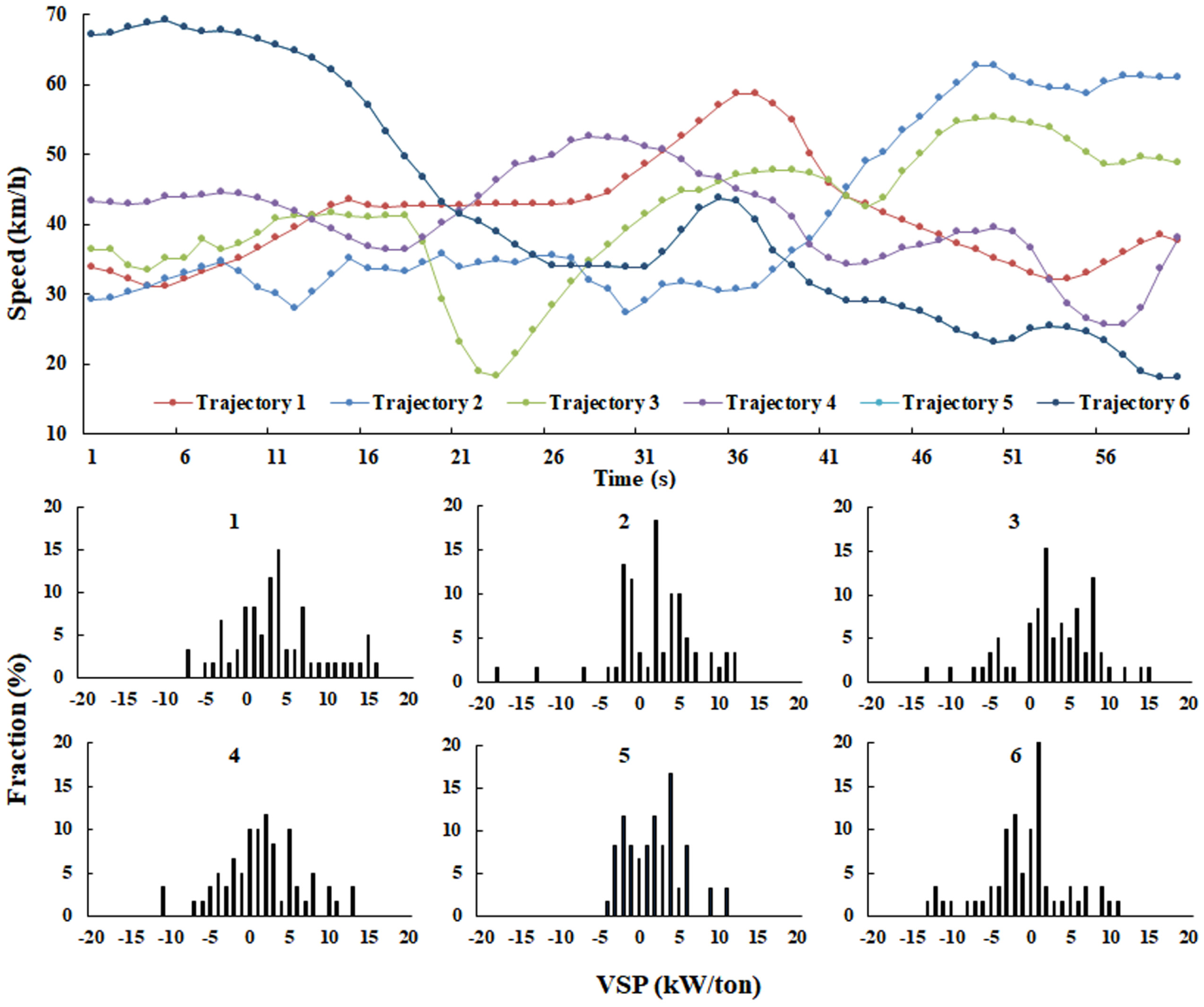
Trajectories and VSP distributions in the same FaSS traffic situation (average speed = 40 km/h on expressways).

Literature Review

VSP is defined as the instantaneous tractive power per unit vehicle mass, in kW/tons ( 6 ). In the MOVES, the VSP distributions are generated by using vehicle activity data, categorized into VSP bins. And VSP distribution is defined as the time (or time fraction) spent in each VSP bin ( 1 ).

To estimate emissions more accurately, many studies focused on the characteristics of VSP distributions. Frey et al. investigated how VSP distributions showed high similarity in the [30, 40] km/h average speed range on different roads ( 7 ). Younglove et al. developed five different types of driving cycles and VSP distributions from conservative to radical ( 8 ). Song et al. developed the relationship between average speed and VSP distribution quantitatively, and developed VSP distributions for different speeds in Beijing ( 3 , 9 ). Wang examined the characteristics of operating mode distributions of different freeway weaving configurations based on a simulation environment ( 10 ). Faced with various traffic conditions, Song et al. developed a series of models and algorithms to estimate fuel consumption ( 11 ). Zhai et al. found that the characteristics of the FaSS VSP distributions were highly consistent temporally and spatially ( 4 ).

Characteristics of developing VSP distributions and estimating emissions change under different driving behavior, vehicle types, and road conditions. Zhao et al. found that characteristics of VSP distributions for heavy-duty vehicles and light-duty vehicles were different in the same average travel speed bin ( 12 ). Jaikumar et al. indicated that emissions for VSP modes under cruising speeds were 10 to 12 times less than under idling, braking, and accelerating conditions ( 13 ). Song et al. observed the characteristics of VSP distributions on urban restricted accessways in Beijing ( 7 ). Zhang et al. analyzed the emissions characteristics for heavy-duty diesel trucks under different loads based on VSP ( 14 ).

Simulation data were also used to describe the traffic operation ( 14 – 16 ). Meanwhile, this sort of technique was questioned on the basis that it could not reflect the real-world traffic situation ( 17 – 19 ). To ensure the accuracy of emission estimation, it is necessary to collect local vehicle activity data. Talbot et al. indicated that the emission estimations derived from using locally developed VSP distributions were significantly improved ( 20 ). Alam et al. illustrated the importance of collecting local bus data when estimating transit bus emissions ( 21 , 22 ). Uncertainty is the possible error in estimating the overall parameters by a sample estimator. The uncertainty of the relationship between VSP distributions and the sample sizes of vehicle activity data for developing VSP distributions determines the accuracy of emission estimating. To eliminate the uncertainty, almost all of the studies collected massive amounts of vehicle activity data. However, Liu implied that a smaller vehicle sample may be enough in relevant research ( 23 ).

To analyze the characteristics of VSP distributions, local vehicle activity data were widely collected to develop local VSP distributions. However, most of the studies collected redundant vehicle activity data. In this context, the primary objective of this study is to quantify the relationship between sample size and the accuracy of developing FaSS VSP distributions for estimating emissions. The rest of this paper is organized as follows. The next section describes the method to develop the FaSS VSP distribution based on real-world second-by-second vehicle activity data. Then the uncertainty of FaSS VSP distributions for a specific traffic situation is investigated. Finally, the relationship between sample size and the accuracy of emission estimation is discussed.

Methodology

The framework of this study is shown in Figure 2. To develop robust FaSS VSP distributions, massive amounts of second-by-second vehicle activity data are collected to reflect various traffic situations. The activity data are divided into pieces of trajectories, each of which consists of 60 s of continuous speed data. The trajectories are categorized into different trajectory pools according to the average speed of each trajectory. FaSS VSP distributions with sample sizes are developed by random sampling of the trajectories from each trajectory pool. The root mean square error (RMSE) is employed to quantify the uncertainty of developing FaSS VSP distributions based on different numbers of trajectories in each trajectory pool ( 4 ). Based on the FaSS VSP distributions at different average speeds, the emission factors are calculated. The minimal sample sizes to develop FaSS VSP distributions for emission estimation are discussed.

Figure 2.

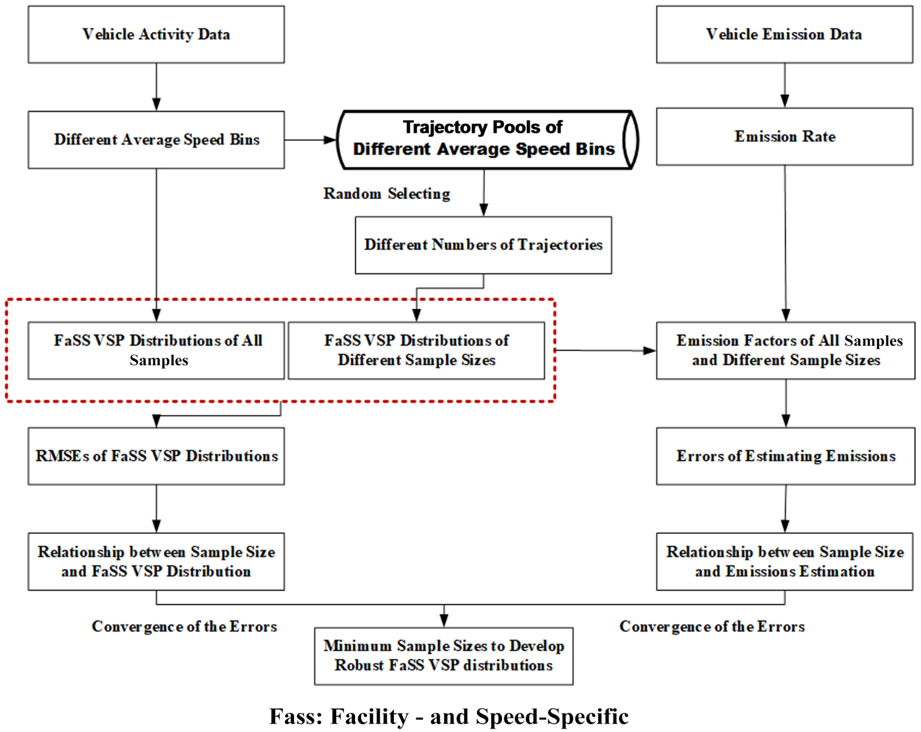
Framework of this study.

Data Sources

To estimate emissions, two kinds of field data are used in this study. The first one is the second-by-second vehicle activity data of light-duty vehicles (LDVs). The activity data are used to develop the FaSS VSP distributions. The second one is the vehicle emission data of LDVs. The emission data are used to obtain the average emissions rates.

Vehicle Activity Data

More than 7.5 million records of second-by-second real-world activity data of LDVs are collected from the Monitoring Platform of Beijing Traffic Energy Saving and Emission. In this paper, the vehicle activity data are matched with the Beijing road network using a geographical information system (GIS). The latitude and longitude are used to identify the road type of the trajectory (expressways or nonexpressways). In this paper, only vehicle movements on the mainline are considered.

The VSP is calculated after data quality control ( 24 ). Other details about the data are as follows:

Collection date: from April 25, 2004 to April 16, 2013.

Collection time: from 5:00 a.m. to 11:00 p.m.

Instantaneous speed: from 0 to 133 km/h, with a precision of 0.1 km/h ( 25 ).

Vehicle Emission Data

The vehicle emissions data are derived from the local emission rates model for light-duty gasoline vehicles ( 26 , 27 ). The emission standard of China III is selected to provide the emission rates for LDVs, because it offers more sufficient data compared with other emission standards. The emission factors based on FaSS VSP are calculated with the following procedures: first, the trajectories are derived from the activity data; second, the FaSS VSP distributions are developed by categorizing the trajectories in the average speed bin; third, the average emission rates in each VSP bin are calculated; and, finally, the emission factors in each average speed bin are calculated.

Developing FaSS VSP Distributions in Different Speed Bins

In this section, the method for developing FaSS VSP distributions is discussed. The activity data are divided into pieces of trajectories, each of which consists of 60 s of continuous speed data. The average speed of each trajectory is calculated. The average speed is divided by 2 km/h and its interval is determined as [0, 2) km/h, [2, 4) km/h, and so forth. Thus, in each average speed bin, the “trajectory pool” represents all of the trajectories. This study selects the average speed bins from [0, 2) km/h to [78, 80) km/h because of the speed limitation on expressways in Beijing.

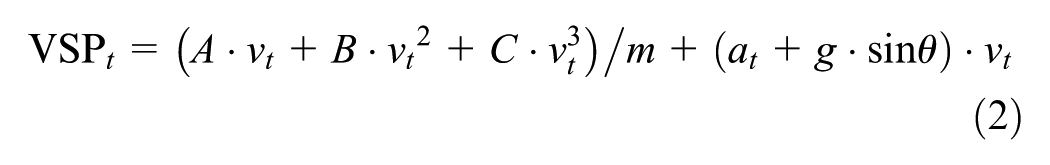
VSP is related to fuel consumption and emissions more closely than to speed and acceleration. The MOVES equations to calculate VSP ( 1 ) are:

a_{t} = v_{t + 1} - v_{t}

(1)

VS P_{t} = (A \cdot v_{t} + B \cdot {v_{t}}^{2} + C \cdot v_{t}^{3}) / m + (a_{t} + g \cdot \sin θ) \cdot v_{t}

(2)

where

v_t, v_t+1 are the vehicle speeds at times t and t + 1, respectively, in m/s;

a_t is the vehicle acceleration at time t, in m/s²;

g is the acceleration resulting from gravity, which is 9.8 m/s²;

sin θ is the road grade;

A, B, C are road load coefficients, representing rolling resistance, rotational resistance, and aerodynamic drag, in the units of kW-s/m, kW-s²/m² and kW-s³/m³, where kW-s represents a kilowatt second, respectively; and

m is the vehicle weight, in metric tons.

The VSP values are calculated using Equation 2. The values of A, B, C, and m are 0.156461, 0.0020002, 0.000493, and 1.4788, respectively ( 28 ).

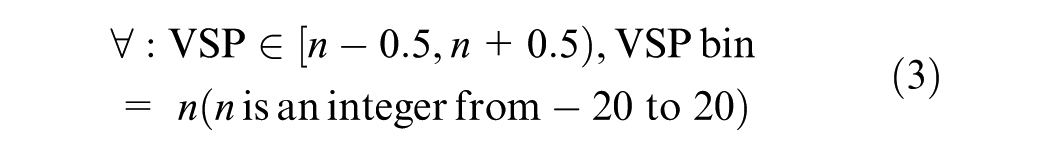
The VSP values are categorized into VSP bins. VSP bins are defined using an equal VSP interval of 1 kW/ton ( 3 ), as shown in Equation 3. It is found that over 98.8% of the VSP values are between −20 and 20 kW/ton ( 3 ), so the analysis in this study focuses on the VSP range of [−20, 20] kW/ton:

\begin{matrix} \forall : VSP \in [n - 0.5, n + 0.5), VSP bin \\ = n (n is an integer from - 20 to 20) \end{matrix}

(3)

For each speed bin, the FaSS VSP distributions are developed by applying the VSP binning method introduced above. The VSP distributions in the average speed bins of [20, 22) km/h, [40, 42) km/h, and [60, 62) km/h for the expressway are presented as examples in Figure 3a.

Figure 3.

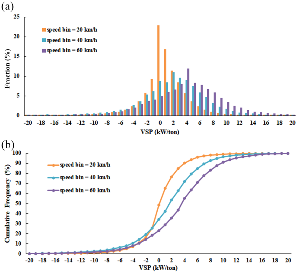
FaSS VSP distributions in different average speed bins.

As shown in Figure 3a, the FaSS VSP distributions vary significantly across different average speeds. The peak value of the VSP distribution keeps decreasing and moving right with the average speed increasing. Figure 3b indicates a cumulative frequency of different FaSS VSP distributions. The VSP fractions are similar when the VSP bin is lower than 0 kW/ton. The VSP values are mostly distributed in the VSP bins of [–2, 2] kW/ton Therefore, it is necessary to investigate the uncertainty of FaSS VSP distribution in different average speed bins.

Developing FaSS VSP Distributions for Different Sample Sizes

In this section, the characteristics of the FaSS VSP distributions developed from different sample sizes are discussed. The sample size refers to the number of trajectories in each trajectory pool. To analyze the relationship between the sample sizes and the robustness of developing FaSS VSP distributions, a true value is needed in each speed bin. In this paper, for each speed bin, the FaSS VSP distributions of all trajectories are developed as the true value. The vehicle activity data are categorized according to the average speed of trajectories, as shown in Table 1. For each speed-specific trajectory pool, multiple sets of FaSS VSP distributions are developed based on various sample sizes.

Table 1.

Sample Sizes of Trajectories in Different Speed Bins

Speed bin (km/h)	Record(s)	Number of trajectories
0	87,043	1,451
2	29,316	489
4	29,553	493
6	35,184	587
8	39,871	665
10	42,863	715
…	…	…
40	31,068	520
…	…	…
70	29,765	497
72	25,396	424
74	24,887	415
76	15,173	253
78	13,430	224

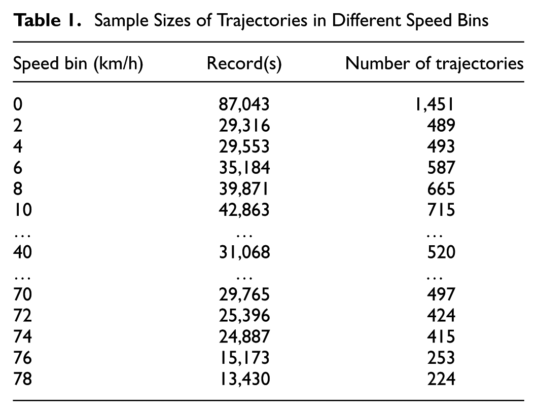
Figure 4 illustrates the FaSS VSP distributions developed from different numbers of trajectories in the speed bin of [40, 42) km/h. The red lines represent the VSP distributions developed from all trajectories. The VSP distributions developed from low numbers of trajectories (e.g., one or two trajectories) are obviously different compared with the VSP distributions of all trajectories. However, the differences between the VSP distributions developed from part and all of trajectories tend to be smaller with the number of trajectories increasing. This is easy to understand because the VSP distribution is developed to represent the average vehicle activities on roads for a specific traffic situation. When the sample size is low, the VSP distribution cannot cover all the activity characteristics for most of the vehicles. When the sample size is large enough, most of the activity characteristics can be covered. The differences in distributions indicate the lack of robustness of developing FaSS VSP distributions from different sample sizes. Thus, the next step is to analyze the minimal numbers of trajectories from the trajectory pool of each speed bin required to develop robust FaSS VSP distributions.

Figure 4.

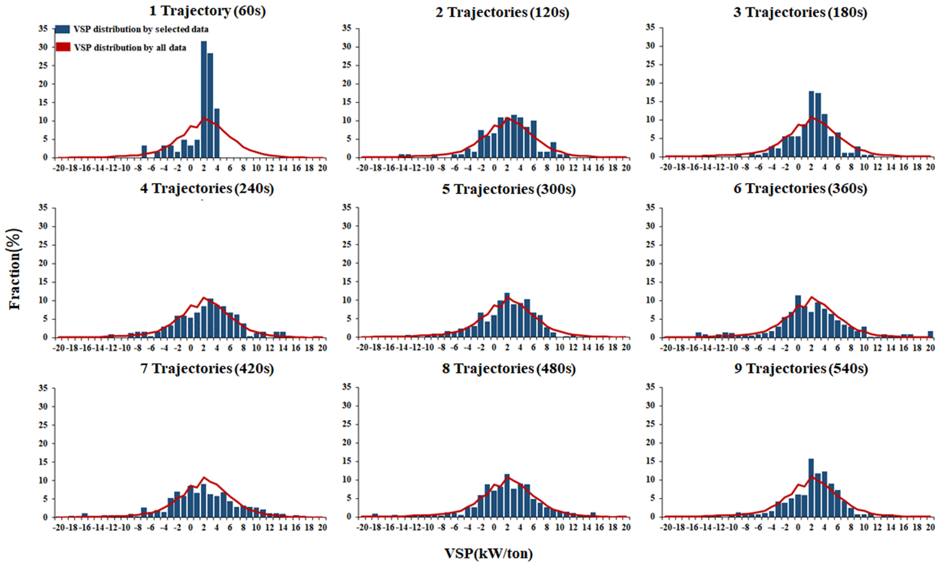
FaSS VSP distributions of different numbers of trajectories in (40, 42) km/h speed bin.

Uncertainties of FaSS VSP Distributions and Emission Estimation

It should be noted that various factors have an impact on developing VSP distributions and emission estimation. This paper focuses on the relationship between sample size and the uncertainty of developing VSP distributions, which is quantified by using RMSE.

Sample Size to Develop FaSS VSP Distribution

To estimate emissions accurately, developing robust FaSS VSP distributions is the basic requirement. In this section, the minimal numbers of trajectories needed to develop a robust VSP distribution is discussed.

To eliminate the randomness of selecting data, the method of multiple data extraction for repeated testing is used. The minimal sampling frequency needs to be determined first. It is calculated by:

n = \frac{{(z_{α / 2})}^{2}}{Δ^{2}} [q (1 - q)]

(4)

where z_α_/2 = 1.64, q = 0.5, and Δ = 0.05. In this formula, q is the overall rate; when the value of q cannot be known, the value is set to 0.5. Δ is the estimation error; the value of Δ is set to 5% in this paper. The value of z_α_/2 is set referred to Table 2 ( 29 ).

Table 2.

The Value of Z_α_/2 for Different Confidence Levels

Confidence level	A	α/2	Z _α/2
90%	0.10	0.05	1.645
95%	0.05	0.025	1.96
99%	0.01	0.005	2.58

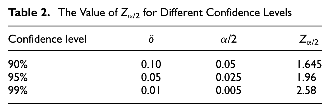
The minimal sampling frequency is calculated to be 269, which means that at least 269 trajectories are randomly selected from each trajectory pool. The sample size is more than 5% of the total data in each trajectory pool. The minimal sampling frequency needs to be adjusted using:

n^{'} = (n \times N) / (n + N - 1)

(5)

where N is the total numbers of trajectories in each trajectory pool.

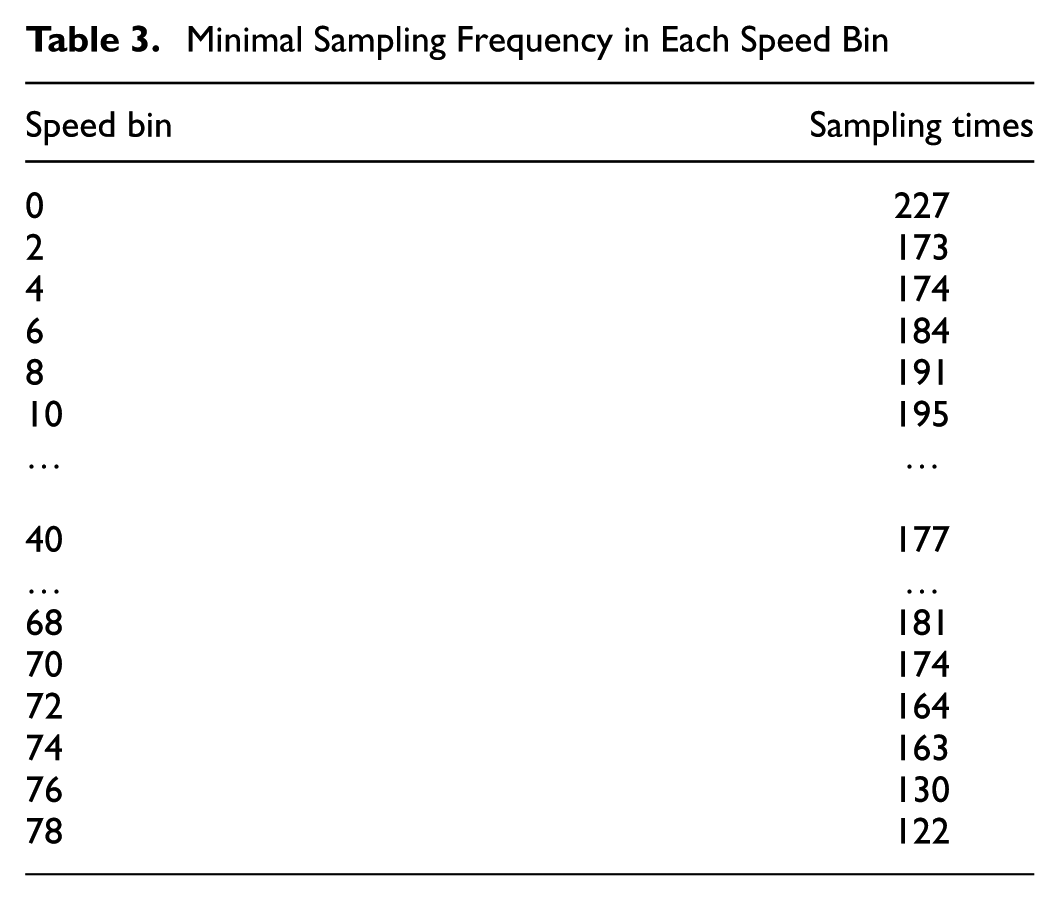
The adjusted minimal sampling frequency in each speed bin is shown in Table 3.

Table 3.

Minimal Sampling Frequency in Each Speed Bin

Speed bin	Sampling times
0	227
2	173
4	174
6	184
8	191
10	195
…	…

40	177
…	…
68	181
70	174
72	164
74	163
76	130
78	122

Trajectories should be randomly selected according to sampling times from each trajectory pool to develop FaSS VSP distributions for each sample size. Meanwhile, the FaSS VSP distributions of all trajectories in each trajectory pool are developed as the true values. To quantify the relationship between sample size and robustness of developing FaSS VSP distributions, RMSE is applied to estimate the uncertainty of the FaSS VSP distributions developed from different numbers of trajectories. The RMSE is calculated by:

RMS E_{a, b} = \sqrt{\sum_{i = 1}^{n} {(φ_{a, i} - φ_{b, i})}^{2} / (n - 1)}

(6)

where

RMSE_a,b is the RMSE of the VSP distribution of a and b;

$φ_{a, i}$ is the fraction of the ith VSP bin in the VSP distribution of a;

$φ_{b, i}$ is the fraction of the ith VSP bin in the VSP distribution of b, which is the VSP distribution developed by all samples; and

n is the number of VSP bins in each VSP distribution, which is 41 in this paper.

According to the requirement of the minimal sampling frequency, FaSS VSP distributions of each sample size are calculated in different speed bins. Then, the RMSEs of FaSS VSP distributions developed from numbers of trajectories and all trajectories are computed for each sample size in each speed bin. To eliminate the impact of abnormal values, the 90th percentile of RMSE is used as the threshold. Figure 5a illustrates the 90th percentile of RMSEs of each sample size in each speed bin. The RMSEs can reach about 16% when low numbers of trajectories are selected. The RMSEs decrease gradually with increasing sample sizes. For each speed bin, the RMSE is lower than 5% when the FaSS VSP distributions are developed from 10 trajectories (600 s) of activity data.

Figure 5.

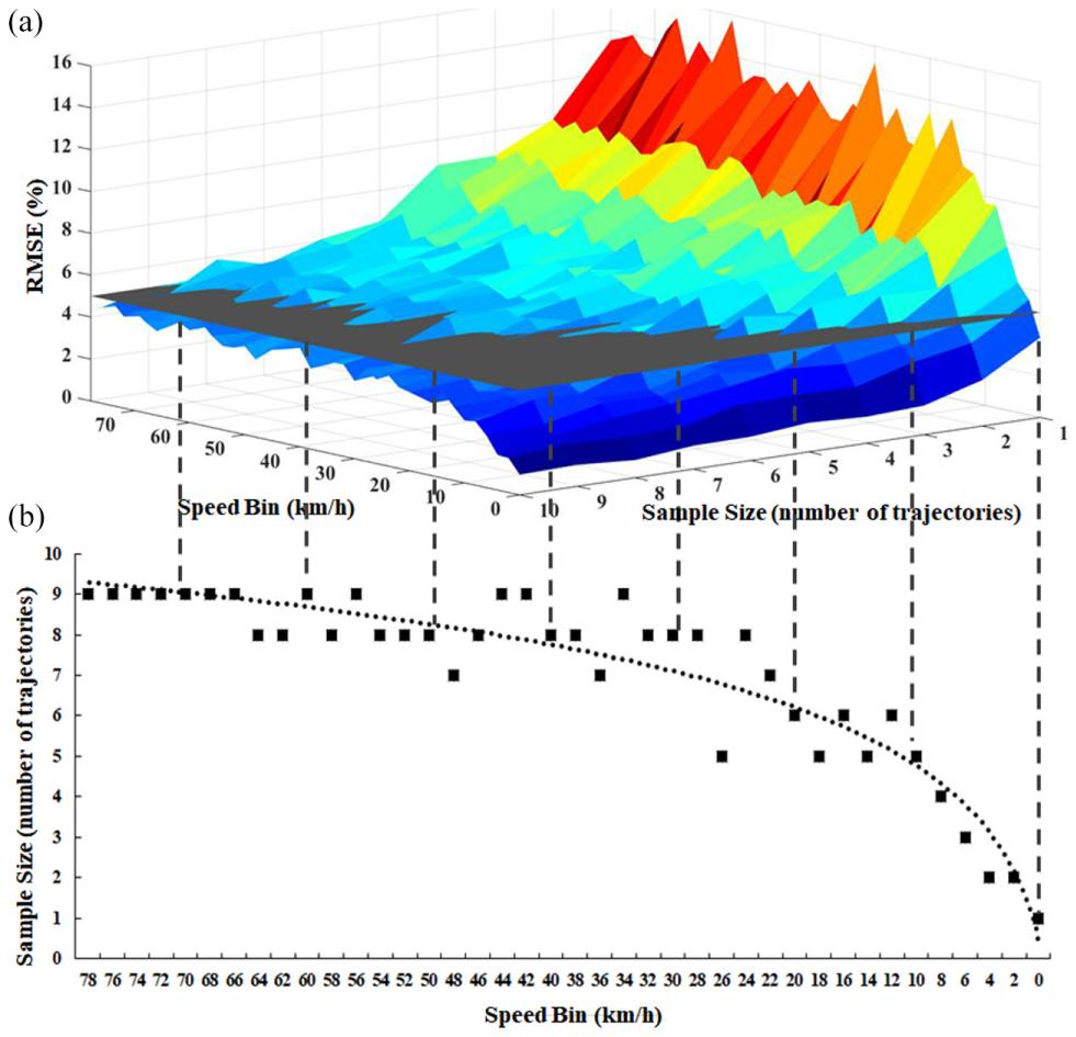
RMSEs of developing FaSS VSP distributions and the trajectories demand with error lower than 5%.

In Figure 5a, the gray surface represents the RMSEs of 5%. The intersection of the error surface and the gray surface is the minimal sample size for developing FaSS VSP distributions with error lower than 5% in each speed bin. Each point in Figure 5b represents the minimal sample size in each speed bin. It is shown that the minimal sample size distribution is similar to a logarithmic distribution. The minimal sample sizes for developing FaSS VSP distributions with error lower than 5% in different speed bins are obviously different. One trajectory (60 s) is needed to satisfy the error requirement in the speed bin for 0 km/h. However, nine trajectories (540 s) are needed in the speed bin for 78 km/h. Nine trajectories (540 s) of vehicle activity data are enough to develop FaSS VSP distributions in each speed bin with error lower than 5%.

To analyze the convergence of RMSEs, the RMSE distributions of 10 speed bins are selected, as shown in Figure 6. It can be visually observed that the RMSEs of FaSS VSP distributions developed from the same sample size are greater in high speed bins. This is because VSP values are concentrated at the VSP bin 0 kW/ton mostly at low average speeds. The FaSS VSP distributions are more stable at low average speed. The RMSEs are stable at under 5% when sample size is more than nine trajectories (540 s). Thirty trajectories (1,800 s) are needed when the RMSEs are lower than 2%. This finding is also applicable to other speed bins.

Figure 6.

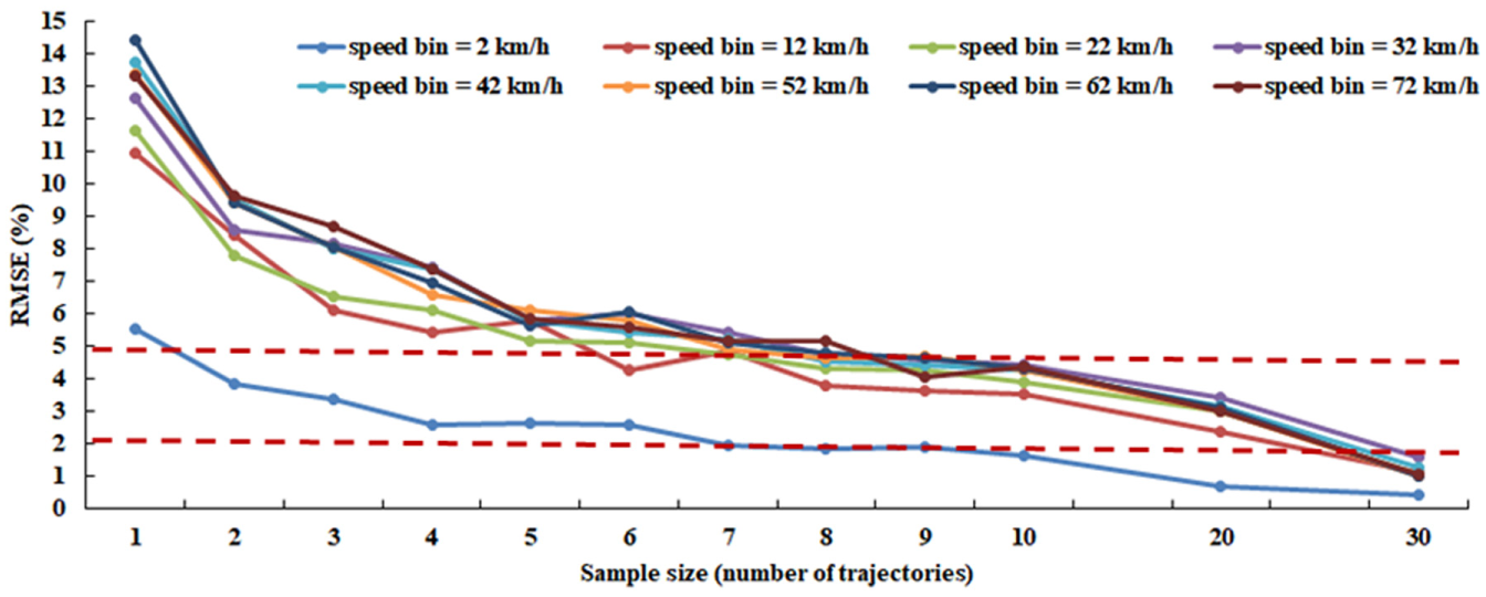
The convergence of the RMSEs of FaSS VSP distributions.

Sample Size to Estimate Emissions Based on FaSS VSP Distributions

The relationship between sample size and the uncertainty of developing VSP distributions has been developed in the above discussion in this paper. In the MOVES model, vehicle emissions are estimated by multiplying the emission rates by the VSP distributions ( 1 ). CO, NO_X, HC and CO₂ (carbon dioxide) emission factors are applied to quantify the relationship between sample size and the accuracy of emission estimation based on VSP. The emission factors are defined as the emissions per unit distance.

The emission factors are calculated using:

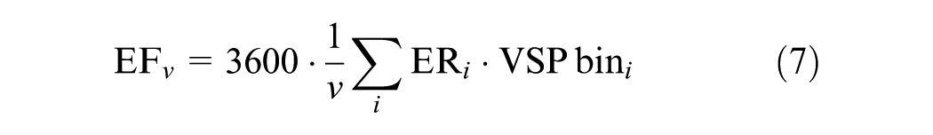
E F_{v} = 3600 \cdot \frac{1}{v} \sum_{i} E R_{i} \cdot VSP bi n_{i}

(7)

where

EF_v is the emission factor in the average speed of ν in g/km;

ν is the average speed, in km/h;

ER_i is the mean emission rate of the ith VSP bin, in g/s; and

VSP bin_i is the time fraction in the ith VSP bin.

Based on the vehicle emission data, the mean emission rates in different VSP bins could be calculated by employing the VSP binning method ( 22 ), as illustrated in Figure 7.

Figure 7.

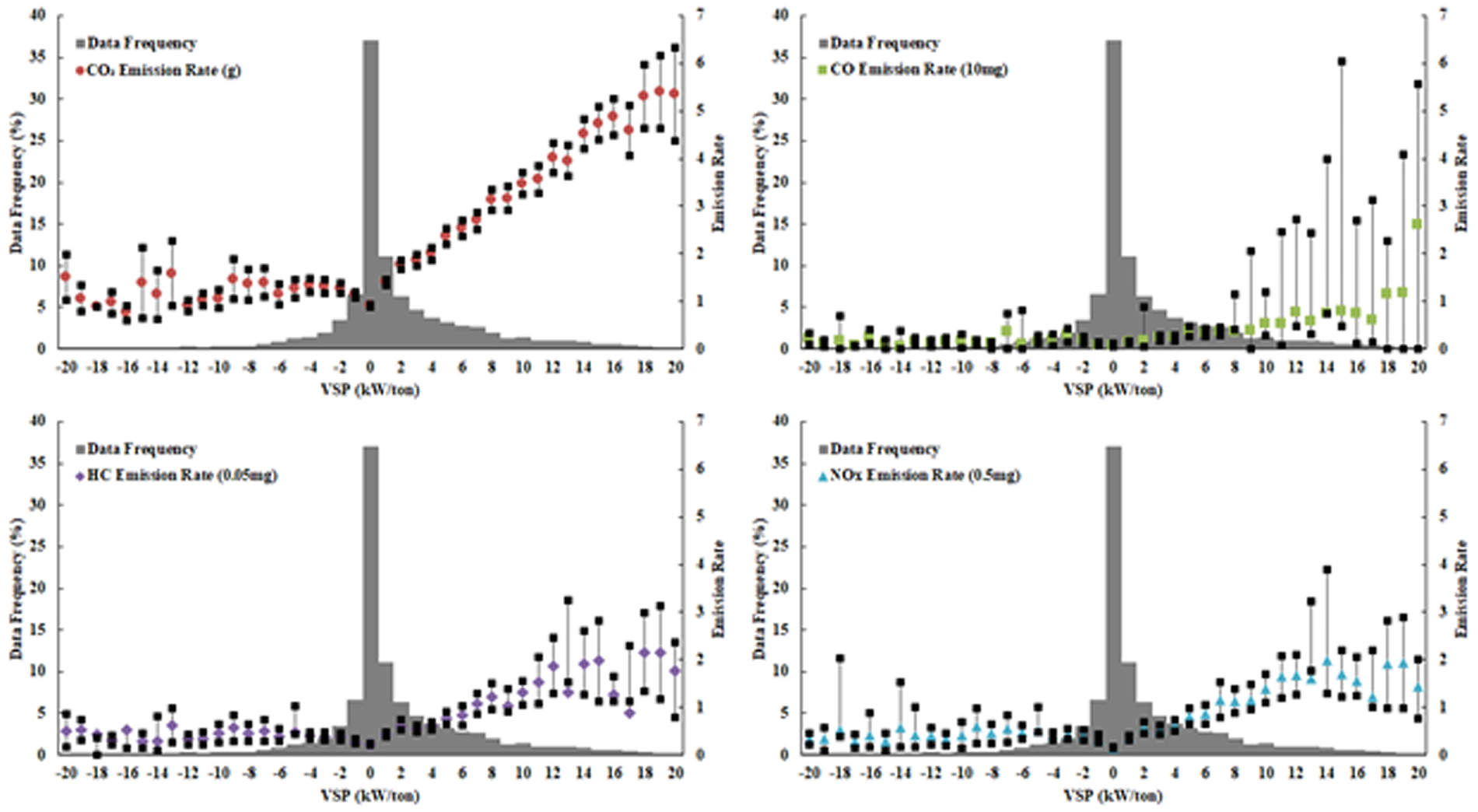
Emission rates and data frequency in each VSP bin.

According to the minimal sampling frequency, the emission factors of each pollutant derived from the FaSS VSP distributions of different sample sizes in each speed bin are calculated separately. The emission factors derived from the FaSS VSP distributions of all trajectories in each trajectory pool are calculated for comparison. The relative errors of estimating emission factors of different sample sizes are calculated. Figure 8 illustrates the 90th percentile of estimating errors of each sample size in each speed bin. The gray surfaces represent an error of 5%. The errors of CO and HC emission factor estimation are greater than those for CO₂ and NO_X when the sample size and speed bin are the same. The errors of all of the pollutants can reach about 30% when VSP distributions are developed from low sample sizes. The errors decrease gradually with increasing sample size. The intersections of the error surfaces and the gray surfaces are the sample sizes for estimating emission factors of each pollutant with an error lower than 5% in each speed bin. The estimation errors are mostly under 5% when the sample size reaches 30 trajectories (1,800 s).

Figure 8.

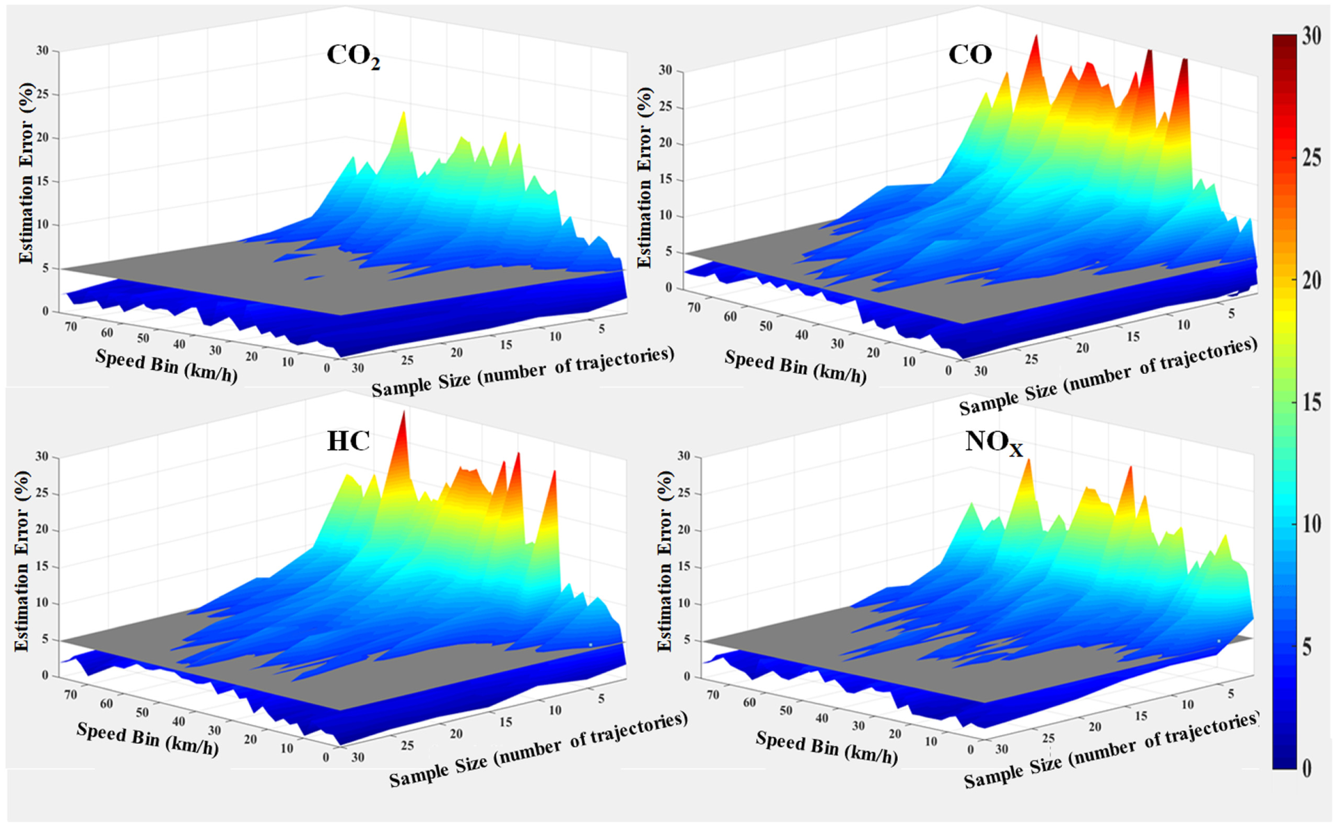
The 90th percentile of emission estimation errors.

Figure 9 illustrates the convergence of emission estimation errors in different speed bins. The errors decrease rapidly when the sample sizes are of fewer than 10 trajectories (600 s). The emission estimation errors are stable at under 5% when the sample sizes are more than 35 trajectories (2,100 s). The finding is also applicable to other speed bins. The errors in different speed bins converge gradually with the sample size increasing.

Figure 9.

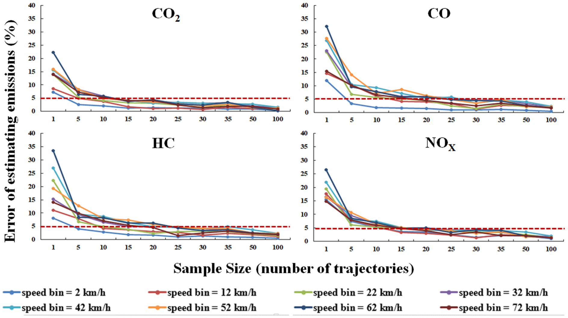
The convergence of emission estimation errors.

The 90th percentile of the relative errors is used as the threshold to eliminate the impact of abnormal values. Figure 10a illustrates the sample sizes to estimate different emission factors with an error lower than 5% in each speed bin. For each speed bin, the sample size to estimate CO₂ emission factors is lowest. To calculate CO₂ emission factors with the calculation error under 5%, 16 trajectories (960 s) of vehicle activity data are enough. Further, the error of calculating CO₂ emission factors is lower than 5% when the RMSEs of developing FaSS VSP distributions converge to 2%. More sample sizes are needed to estimate emission factors of CO, NO_X, and HC in each speed bin. Thirty-five trajectories (2,100 s) are enough to estimate emissions with an error lower than 5% for each pollutant in each speed bin.

Figure 10.

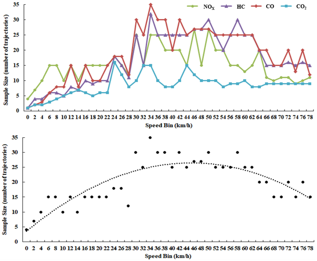
Sample sizes to develop FaSS VSP distributions for emissions estimation with an error lower than 5% for a 90% confidence level.

Different sample sizes are needed to calculate emission factors for CO₂, CO, NO_X, and HC in each speed bin. The biggest sample size to calculate different emission factors in each speed bin is selected as the minimal sample size to estimate emissions satisfying the requirement of 5% error. As shown in Figure 10b, the point in each speed bin represents the minimal sample size. The minimal sample size distribution is similar to a polynomial distribution. When the average speed is between 30 and 40 km/h, the sample demand is larger than for other speed bins.

Comparing with the minimal sample size to develop robust FaSS VSP distributions, more samples are needed to ensure the accuracy of estimating emissions. For a robust FaSS VSP distribution, the fraction in each VSP bin is relatively fixed. For emissions, the fractions change dramatically in different VSP bins. As introduced above, the MOVES model calculates emission factors by multiplying the emission rates by the VSP distributions. This calculation method equates to multiplying the fraction in each VSP bin by a weight coefficient when multiplying the emission rates. Therefore, it is inferred that this calculation method causes an increase in the uncertainty of emission estimation.

Conclusions and Recommendations

In this paper, the sample size of vehicle activity data is analyzed for improving accuracy of emission estimation. More than 7.5 million items of second-by-second vehicle activity data in the real world are collected and divided into various “trajectory pools” according to the average speed. The FaSS VSP distributions of different numbers of trajectories in each trajectory pool are developed. The emission factors of CO₂, CO, NO_X, and HC are calculated based on the VSP distributions of different sample sizes. The main findings are summarized as follows:

For each FaSS traffic situation, the more trajectories, the more robust the FaSS VSP distributions of the trajectory pool are. When the errors are lower than 5%, nine trajectories (540 s) are needed to develop FaSS VSP distributions for a 90% confidence level. The errors of developing FaSS VSP distributions converge to 2% when the sample size reaches 30 trajectories (1,800 s) for a 90% confidence level, which means the errors of calculating fuel consumption and greenhouse gas (GHG) emissions are lower than 5% for a 90% confidence interval.

To ensure the accuracy of estimating emissions of CO, NO_X, and HC based on VSP distributions, at least 35 trajectories (2,100 s) of vehicle activity data are needed to develop FaSS VSP distributions with estimation error lower than 5% for a 90% confidence level. Because the FaSS VSP distributions developed by 60-s trajectories and 120-s trajectories are identical ( 30 ), 18 120-s trajectories of vehicle activity data satisfy the data demand to estimate emissions.

The study implies that it is unnecessary to collect redundant activity data for estimating emissions. In this paper, the relationship between the sample size and uncertainty of estimating emissions on expressway is developed. Further study is needed to develop the relationship between the sample size and the emission estimation on nonexpressway. The uncertainty of estimating emissions of other vehicle types also needs to be analyzed.

Footnotes

Acknowledgements

This research was supported by the Natural Science Foundation of China (NSFC) # 51678045 and 51578052, the Fundamental Research Funds for the Central Universities # 2018YJS081, and Henan Provincial Department of Transportation Program # 2018G3. The authors are grateful to all the personnel who either provided technical support or helped with data collection and processing.

Author Contributions

The authors confirm contribution to the paper as follows: study conception and design: Z. Zhang, G. Song; data collection: Z. Zhai; analysis and interpretation of results: Z. Zhang, G. Song, C. Li, Y. Wu; draft manuscript preparation: Z. Zhang, G. Song. All authors reviewed the results and approved the final version of the manuscript.

The Standing Committee on Transportation and Air Quality (ADC20) peer-reviewed this paper (19-02780).

References

Population and Activity of On-Road Vehicles in MOVES2014 . EPA-420-R-16-003a. Environmental Protection Agency, Washington, D.C., 2016.

Song

Sensitive Analysis of Emission Rates in MOVES for Developing Site-Specific Emission Database. Transportation Research Part D: Transport and Environment, Vol. 32, 2014, pp. 193–206.

Song

Characteristics of Low-Speed Vehicle-Specific Power Distributions on Urban Restricted-Access Roadways in Beijing. Transportation Research Record: Journal of the Transportation Research Board, 2011. 2233: 90–98.

Zhai

Song

Validation of Temporal and Spatial Consistency of Facility- and Speed-Specific VSP Distribution for Emission Estimation: A Case Study in Beijing. Journal of the Air & Waste Management Association, Vol. 67, 2017, pp. 949–957.

Vehicle Operating Mode Distribution Model for Emission Evaluation on Traffic Networks. PhD dissertation. Beijing Jiaotong University, Beijing, China, 2011.

Jiménez-Palacios

J. L

. Understanding and Quantifying Motor Vehicle Emissions with Vehicle Specific Power and TILDAS Remote Sensing. PhD dissertation. Massachusetts Institute of Technology, Cambridge, MA, 1999.

Frey

H. C.

Rouphail

N. M.

Zhai

Speed- and Facility-Specific Emission Estimates for On-Road Light-Duty Vehicles on the Basis of Real-World Speed Profiles. Transportation Research Record: Journal of the Transportation Research Board, 2006. 1987: 128–137.

Younglove

Scora

Barth

Designing On-Road Vehicle Test Programs for the Development of Effective Vehicle Emission Models. Transportation Research Record: Journal of the Transportation Research Board, 2005. 1941: 51–59.

Song

Distribution Characteristics of Vehicle-Specific Power on Urban Restricted-Access Roadways. Journal of Transportation Engineering, Vol. 138, 2011, pp. 202–209.

10.

Wang

Rakha

H. A.

Operating Mode Distribution Characteristics of Different Freeway Weaving Configurations and Their Effects on Vehicular Emissions. Presented at 93rd Annual Meeting of the Transportation Research Board, Washington, D.C., 2014.

11.

Song

Development of Fuel Consumption and Vehicle Emission Models for Evaluation of Transportation Strategies [in Chinese]. PhD dissertation. Beijing Jiaotong University, Beijing, China, 2008.

12.

Zhao

Song

Characteristics of VSP Distributions of Light-Duty and Heavy-Duty Vehicles on Freeway: A Case Study. Presented at 91st Annual Meeting of the Transportation Research Board, Washington, D.C., 2012.

13.

Jaikumar

Nagendra

S. M. S.

Sivanandan

Modeling of Real Time Exhaust Emissions of Passenger Cars under Heterogeneous Traffic Conditions. Atmospheric Pollution Research, Vol. 8, 2017, pp. 80–88.

14.

Farzaneh

Pesti

Valdez

Birt

Estimating Vehicular Emission Impact of Nighttime Construction with Vissim and Different MOVES Emission Estimation Approaches. Transportation Research Record: Journal of the Transportation Research Board, 2018. 2672(25): 174–186.

15.

Abou-Senna

Radwan

VISSIM/MOVES Integration to Investigate the Effect of Major Key Parameters on CO₂ Emissions. Transportation Research Part D: Transport and Environment, Vol. 21, 2013, pp. 39–46.

16.

van Zuylen

Chen

Viti

Wilmink

Optimizing Traffic Control for Emissions with a Valid Simulation Program—The Calibration of a Simulation Model for Emission Estimation. Presented at 90th Annual Meeting of the Transportation Research Board, Washington, D.C., 2011.

17.

Zhang

Song

Emissions Characteristics for Heavy-Duty Diesel Trucks under Different Loads Based on Vehicle-Specific Power. Transportation Research Record: Journal of the Transportation Research Board, 2017. 2627: 77–85.

18.

Song

Geng

Optimization of Wiedemann and Fritzsche Car-Following Models for Emission Estimation. Transportation Research Part D: Transport and Environment, Vol. 34, 2015, pp. 318–329.

19.

Cui

Choi

Park

B. B.

Ryu

Field Evaluation of Vehicle-to-Infrastructure Communication-Based Eco-Driving Guidance and Eco-Signal System. Transportation Research Record: Journal of the Transportation Research Board, 2018. 2672(25): 123–138.

20.

Talbot

Chamberlin

Holmén

B.A.

Sentoff

Calibrating a Traffic Microsimulation Model to Real-World Operating Mode Distributions. Presented at 93rd Annual Meeting of the Transportation Research Board, Washington, D.C., 2014.

21.

Alam

Hatzopoulou

Deriving Local Operating Distributions to Estimate Transit Bus Emissions across an Urban Network. Transportation Research Record: Journal of the Transportation Research Board, 2016. 2570: 57–68.

22.

Alam

Hatzopoulou

Modeling Transit Bus Emissions using MOVES: Validation of Default Distributions and Embedded Drive Cycles with Local Data. Presented at 94th Annual Meeting of the Transportation Research Board, Washington, D.C., 2015.

23.

Liu

Hatzopoulou

Measurement and Evaluation of Real-World Light-Duty Vehicle Speed and Acceleration Activity Envelope. Transportation Research Record: Journal of the Transportation Research Board, 2015. 2503: 128–136.

24.

Report of Overall Architecture Design and Technical Difficult of the Distribution Regular Pattern of Traffic Emissions . Technical Report for Center for Transportation Sector Energy Reduction and Emissions Mitigation of Beijing, Beijing Jiaotong University, Beijing, China, 2014.

25.

Zhang

Guo

Cheng

Song

Optimized Adjustment of Speed Resolution and Time Alignment Data for Improving Emission Estimations. Transportation Research Record: Journal of the Transportation Research Board, 2016. 2570: 77–86.

26.

Xie

Song

Guo

Sun

Development and Application of an Online Dynamic Emission Model for Traffic Networks: A Case Study of Beijing. Presented at 97th Annual Meeting of the Transportation Research Board, Washington, D.C., 2018.

27.

Cheng

Song

Development of Local Emissions Rate Model for Light-Duty Gasoline Vehicles: Beijing Field Data and Patterns of Emissions Rates in EPA Simulator. Transportation Research Record: Journal of the Transportation Research Board, 2017. 2627: 67–76.

28.

MOVES2010 Highway Vehicle Population and Activity Data . EPA-420-R-10-026. Environmental Protection Agency, Washington, D.C., 2010.

29.

Statistics [in Chinese]. China Renmin University Press, Beijing, China, 2000, pp. 159–180.

30.

Cheng

Optimization of Aggregation Level of Floating Car Data for Estimation of Fuel Consumption and Emissions [in Chinese]. MS dissertation. Beijing Jiaotong University, Beijing, China, 2011.

Speed bin	Sampling times
0	227
2	173
4	174
6	184
8	191
10	195
…	…

40	177
…	…
68	181
70	174
72	164
74	163
76	130
78	122

Speed bin	Sampling times
0	227
2	173
4	174
6	184
8	191
10	195
…	…

40	177
…	…
68	181
70	174
72	164
74	163
76	130
78	122

Speed bin	Sampling times
0	227
2	173
4	174
6	184
8	191
10	195
…	…

40	177
…	…
68	181
70	174
72	164
74	163
76	130
78	122