Impact of Bus Routes on Crash Frequency in Metropolitan Areas

Abstract

Although research in transportation safety is abundant, very few studies have examined the relationship between public transportation systems and safety performance. Most studies on the subject have focused on the impact of infrastructure countermeasures related to bus rapid transit systems. However, the impact of city-street buses on safety performance remains unknown. This research explores the pseudo-causal impact of the presence of bus routes and bus traffic on observed crash frequencies by developing safety performance functions (SPFs) that include the presence of a bus route and estimated weekly bus traffic as input variables. The SPFs were developed using the propensity score–potential outcomes (PS-PO) framework to reduce unobserved biases that might exist between segments that have and do not have bus routes. The results suggest that PS-PO reduced standardized biases significantly, allowing stronger causal inferences to be obtained. The results revealed that the presence of a bus route was associated with a 27% increase in expected crash frequency after controlling for other infrastructure-related variables. Weekly bus traffic was also found to be a significant predictor of overall crash frequency, with a 1% increase in ] weekly bus traffic associated with an expected increase in crash frequency of 0.016%. A non-parametric approach is also presented for comparison with the results from the SPFs; this confirmed the findings from the parametric method used.

The American Association of State Highway and Transportation Officials (AASHTO) Highway Safety Manual (HSM) ( 1 ) provides a set of tools that allows a user to predict the safety performance of roadway elements as a function of infrastructure features, environmental conditions, and traffic exposure for different roadway types. These tools include safety performance functions (SPFs)—models that provide predictions for safety performance as a function of explanatory variables under some baseline conditions—and crash modification factors (CMFs)—adjustments that can be applied to SPFs for cases in which the baseline conditions are no longer valid. Both SPFs and CMFs are statistically derived functions that reveal relationships between safety performance and variables of interest. However, these tools have several limitations, one of which is that they are only focused on total vehicle crashes and, to a lesser extent, pedestrian and bicycle crashes. In general, very little attention has been paid in the HSM to the relationship between public transportation service and safety performance.

Public transportation serves as a sustainable, equitable, and cost-effective alternative to private vehicles. This is largely owing to the lower space efficiency and high societal costs associated with the parking of private vehicles, particularly in medium-to-large cities where high congestion levels are common. However, buses travel more slowly than other vehicles, have reduced acceleration/deceleration capabilities, and frequent stop-making behavior that may increase the lane changing patterns of other vehicles, all of which tends to generate long queues of general traffic behind buses and may increase unexpected swerving maneuvers, thus reducing the safety performance of segments where bus routes are present. This increases the likelihood of a crash occurrence given that other vehicles in the traffic must be more situationally aware and cautious while driving behind buses compared with driving in homogenous traffic environments.

Bus crashes not only have high emotional and economic costs for the individuals involved but for society as a whole in the form of indirect costs as a result of congestion delay. These costs vary considerably according to the severity of crashes and roadway traffic conditions. For instance, even property-damage crashes along major arterials can have high costs during peak hours.

Although crash frequency modeling in traffic safety literature is rich and diverse overall, very few studies focus on the relationship between public transit and road safety ( 2 ). Furthermore, those that focused on ground public transit examined the impact of specific transit infrastructure improvements [e.g., guardrails to prevent jaywalking on light rail corridors or dedicated bus lanes ( 3 ) and protected phases for left turns that have to cross bus rapid transit (BRT) lanes with priority ( 4 )] on road safety rather than the impact of a bus route without isolating the infrastructure. Although various studies have suggested safety countermeasures for transit, there is little quantitative evidence on their effectiveness ( 5 ). Most studies have focused on light rail transit ( 5 ) and those that do consider buses have primarily focused on BRT systems ( 3 – 7 ).

Some of these studies have used simple percentage comparisons or descriptive analyses of crash frequency by transport mode ( 8 ) or before and after scenarios from the implementation of BRT systems ( 6 ). More advanced studies have developed statistical models, for example, negative binomial ( 3 , 7 ) and mixed effects negative binomial models ( 9 ). These studies have found that the implementation of infrastructure related to BRT systems (e.g., rightmost lanes dedicated to bus lanes without physical division that act as a buffer for runaway crashes, and separated bus corridors that also serve as a median) reduces crash frequencies in the corridors where buses previously shared the road with other types of vehicles ( 3 – 7 ). However, novel types of crashes may occur as a result of the new traffic conditions that these infrastructure elements generate. For example, some areas around the busiest stations experienced an increase in crash frequency because of higher traffic speeds produced by the removal of traffic lights ( 3 , 5 ).

Some studies have implemented qualitative approaches to evaluate the factors that increase the risk of a crash, particularly with a focus on the effect of the driver. These studies have collected data using surveys and interviews ( 3 , 10 – 13 ). Statistical methods, such as structural equation modeling, can then be used to analyze attitudes and personality traits ( 10 , 11 ). These studies have revealed fairly intuitive relationships ( 11 ); for example, altruism correlates positively with traffic safety, whereas attitudes like excitement-seeking and normlessness (the individual’s belief that to accomplish a goal, one does not necessarily need to adhere to the rules) are significant predictors of a higher crash risk ( 10 ). However, the use of qualitative methods means that these results cannot be used to quantify the impacts of these features on observed crash frequencies. Fatigue and the severe sleepiness of city bus drivers have also been studied using logistic regression and predictors related to the physical and biological background of the driver, sleep and health indices, and related working experience ( 12 ). Other aspects such as rural immigration to cities, and poor transportation systems were qualitatively found to contribute to bus-related crashes ( 13 ).

The majority of these studies have taken place in under-developed or developing countries where traffic conditions may differ significantly from developed countries ( 3 , 6 , 8 , 11 , 13 ). Only a few studies used data from developed countries, where conditions are comparable with the United States ( 7 , 9 – 12 ).

Overall, there is very limited research that has examined the causal impact of buses on traffic crashes in the United States. The present study aimed to address this literature gap by assembling a database of transit-related crashes in Pennsylvania and undertaking a causal inference analysis by treating the presence of bus routes along a roadway segment as a “treatment” variable. To do this, the propensity score–potential outcomes (PS-PO) framework was adopted to construct comparable control (without a bus route) and treatment (with a bus route) group samples with respect to multiple control variables. In this context, the objective of the current research was to quantify the impact of bus routes on the frequency of all crashes along road segments in the metropolitan areas of Pittsburgh and Philadelphia. In addition, one of the significant challenges that public transit faces is service reliability. Even small and local disturbances in a complex and non-resilient system like a public bus route can have substantial consequences; specifically, roadway crashes can cause significant delays, re-routing, re-scheduling, and even cancellation of transit services in some circumstances, meaning that even moderate deviations from service schedules can significantly affect user satisfaction and transit ridership ( 14 ). For this reason, this research also provides a brief analysis of crashes that include public buses.

The remainder of this paper is organized as follows. First, the methodology that was used to develop relationships between bus route presence, bus traffic, and safety outcomes are presented. Next, the data used in this work is described, and the results are presented. Finally, the discussion and conclusions are provided.

Methodology

This section describes the methods used to analyze crash data in this study. First, spatial methods were used to assemble the modeling database. The PS-PO framework was then applied to minimize potential biases in the database between roadway segments that do not have bus routes and those that do. Finally, the model used to identify the relationship between bus route presence/bus traffic and safety performance was described. Note that models were estimated using all observations and also only the data identified in the PS-PO framework to quantify the need for this method. In general, identifying segments with and without bus routes that have similar conditions and infrastructure treatments should provide confidence that differences in safety performance are highly related to the presence of a bus route or bus traffic.

Spatial Procedures

One of the first data processing tasks was to link each record in the crash database to exactly one of the bus routes. To do this, spatial tools were used to append crash records to bus routes based on spatial proximity. First, using crash coordinates, each crash record was mapped to the metropolitan area where the bus service was offered.

Next, a small buffer region was created around each road segment to allow some tolerance while overlaying crash records. Specifically, a buffer of 100 ft was used to account for GPS accuracy as well as to include segments with multiple lanes where it is very common for buses to move through the rightmost lane (instead of the roadway centerline, simplified by the spatial data). Visual inspection was also used to verify that the buffer region selected was not so large that crashes outside of bus routes would be incorrectly matched. The weekly bus traffic along each roadway segment was obtained by aggregating the weekly traffic for all bus lines that ran through that segment.

All the spatial visualization and editing operations were implemented using the open-source software QGIS (QGIS Development Team) ( 15 , 16 ). All shapefiles were used under the NAD83 (North American Datum) Pennsylvania South (ftUS) projection. This is particularly relevant given that spatial algorithms were implemented with multiple layers and their projections and references must match to avoid inaccurate results.

After the spatial join, each segment not only had the roadway geometry information from the original roadway database but also an indicator variable for the presence of a bus route, the weekly bus traffic, and the number of crashes that occurred along that segment. Furthermore, a new variable was created to differentiate the segments from the different regions where that data were obtained (specifically, the cities of Pittsburgh and Philadelphia) to examine the potential for regional differences in safety performance.

Propensity Scores–Potential Outcome (PS-PO) Framework

In this study, the authors define the causal effect of bus routes on traffic safety as the change in the expected number of crashes when there is a bus route along a segment and the expected number of crashes where there is no bus route present. One of the fundamental challenges associated with inferring this causal effect is that we can only observe the outcome variable (crash frequency) for the treatment received (i.e., whether there is a bus route or not) for any given segment. For the same segment, we cannot observe the crash frequency for both with and without a bus route. However, the average causal effect across the population can be estimated by constructing pseudo-samples with comparable distributions of covariates in the two groups: segments with and without bus routes.

Crash frequency models, referred to as SPFs in the safety literature, were developed by pooling the control (i.e., non-bus route) and treatment (i.e., bus route) group samples to estimate the impact of bus traffic on crashes ( 17 – 19 ). The PS-PO method was used to consider the presence of a bus route as a treatment and evaluate its effect on crash frequency ( 20 ), while controlling for other road geometry variables ( 17 ). The PS-PO framework has previously been applied in the field of transportation to estimate SPFs and CMFs related to signal installation ( 21 ), retroreflectivity of pavement markings for nighttime crashes ( 22 ), design exceptions on non-freeway segments ( 23 ), differences in crash severity levels between lighted and unlighted intersections ( 24 ), lane widths on urban arterials and collectors ( 25 ), and the presence of horizontal curves ( 26 ).

The PS-PO methodology is based on the following assumptions ( 17 , 24 , 27 ):

Stable unit treatment value assumption: This refers to the independence among treated entities, that is, a treatment applied to one segment has no effect on or interaction with any other segment.

Positivity: Each segment has a positive probability (i.e., greater than zero) of receiving the treatment or not, regardless of the observed outcome.

Un-confoundedness: The treatment applied is conditionally independent of the potential outcome, given the set of predictors used to define similarity among segments. It is also assumed that the covariates used already include all possible confounding variables.

To apply the PS-PO method, first a statistical model is estimated that provides each segment with a propensity score. This propensity score is a numerical value that indicates the likelihood that a segment has or does not have the treatment. In this paper, the propensity score was estimated using a simple binary logit model, as presented in Equation 1.

P (B | X_{i} = x_{i}) = \frac{e^{x_{i} β_{i}}}{1 + e^{x_{i} β_{i}}}

(1)

where B is the indicator variable for presence of a bus route along segment i, and x is a vector of infrastructure-related predictors ( 17 ).

This model was used to estimate the propensity score for all segments in the analysis database. Segments in the treated and control groups were then matched using the 1:1 nearest neighbor method with standard Euclidean distance. In this matching procedure, one record in the treatment group is uniquely matched to one record in the control group based on the Euclidean proximity of the propensity score. A 1:1 matching ratio was used because the number of segments that have a bus route (45%) was approximately equal to those without a bus route (55%). Therefore, higher matching ratios would not be possible without discarding observations. A caliper parameter (used as a tolerance measure for dissimilarity when comparing segments) was set to 0.25 times the standard error of the propensity scores obtained in the previous step ( 28 ). Treatment segments for which a control segment did not exist with a propensity score within this caliper range were excluded from further analysis.

The usefulness of propensity score matching can be quantified by estimating the standardized bias for independent variables between treated and controlled segments in the matched and unmatched (i.e., all observations) databases. This standardized bias represents how much bias is present between the treated and control groups. The standardized bias was calculated as presented in Equation 2.

SB = 100 (\frac{({\bar{x}}_{T} - {\bar{x}}_{UT})}{\sqrt{\frac{{s_{T}}^{2} + {s_{UT}}^{2}}{2}}})

(2)

where

SB = the standardized bias for a specific variable,

$\bar{x}$ = the sample means, and

$s^{2}$ = the sample variances.

The subscript T refers to the group with treatment (presence of a bus route in the segment) and the subscript UT denotes the untreated group.

The outcome from propensity score matching is considered successful if the standardized bias is less than 10% in magnitude, meaning that the bias between treated and untreated segments is low ( 17 , 29 ). In such cases, the potential outcomes obtained using statistical models estimated using the sample of matched cases from the PS-PO framework provide more unbiased estimates of the treatment being studied (in this case, the effect of bus traffic on crashes). Crash frequency models on complete unmatched data were also estimated to compare these results with those obtained on the matched dataset, and to evaluate the effect of the balanced presence of a bus route on the estimates from the models.

Crash Frequency Estimation

Potential outcomes are evaluated by estimating a statistical model on the matched database. As crashes are count outcomes by nature, they are often modeled using a Poisson regression framework ( 2 , 30 ).

y_{i} | λ_{i} ~ Poisson (λ_{i})

(3)

where $y_{i}$ is the number of crashes for road segment i, and $λ_{i}$ is the expected crash rate for segment i. Then, the relationship between the explanatory variables and the expected rate is a log-linear model:

λ_{i} = \exp (β_{0} + \sum_{k} β_{k} x_{ik} + ε_{i})

(4)

where

$β_{0}$ = intercept,

$β_{k}$ = coefficient for the $k^{th}$ covariate,

$x_{ik}$ = value of $k^{th}$ covariate for crossing i, and

$ε_{i}$ = heterogeneity among segments.

However, Poisson models cannot handle over-dispersed data in which the variance is greater than the mean value. Such over-dispersion is common when dealing with crash data ( 2 ). Assuming that the heterogeneity term $ε_{i}$ follows a gamma distribution with mean 1 and variance $α$ , leads to the negative binomial (NB) regression ( 30 ), which relaxes the assumption of equal mean and variance in the standard Poisson model. The probability expression of the resulting NB model can be written as shown in Equation 5( 30 ).

P (y_{i}) = \frac{Γ ((1 / α) + y_{i})}{Γ (1 / α) y_{i}!} {(\frac{1 / α}{(1 / α) + λ_{i}})}^{1 / α} {(\frac{λ_{i}}{(1 / α) + λ_{i}})}^{y}

(5)

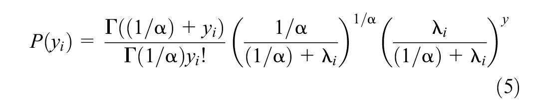
Coefficients of the model were estimated using the maximum likelihood inference method. Coefficients were chosen that maximizee the product of Equation 5 across the individual observations in the estimation sample. Multiple model specifications were tested and compared using the Akaike information criterion (AIC), the Bayesian information criterion (BIC), and p-values, along with domain knowledge in cases when a predictor was not statistically significant at a 95% confidence level. In addition, to determine the relevance of the overdispersion (extra parameter) from the NB model, the likelihood ratio (LR) test statistic of comparison between the Poisson and NB models was computed as

- 2 \times (L L_{Poisson} - L L_{Negative Binomial})

(6)

Data

Crash data for this study were obtained from the Pennsylvania Department of Transportation. The dataset consists of all statewide crashes from 2014 to 2017. Within Pennsylvania, the current study focused on the metropolitan areas of Pittsburgh and Philadelphia because of the relatively high frequency of bus routes and heavy bus traffic compared with the rest of the state. Bus route locations for the Port Authority of Allegheny County (PAAC) in Pittsburgh were obtained through the website from the Western Pennsylvania Regional Data Center, whereas bus routes for the Southeastern Pennsylvania Transportation Authority (SEPTA) in Philadelphia were obtained through the Pennsylvania Spatial Data Access website.

The segments were filtered to keep only those where the presence (or lack thereof) of bus routes could be determined. The population of crashes considered corresponded to those that occurred anywhere in the network, during regular bus service operation hours (between 5 a.m. and midnight) and that resulted in at least one lane closure (because of the impact these crashes might have had on bus services and general traffic operations).

During data assembly, segments with missing values for key explanatory variables were excluded from the analyses. Of those, segments with average annual daily traffic (AADT) less than 50 (0.05% of all roadway segments), those shorter than 250 ft in length (2.3%), and those that were less than 10 ft wide (0.002%) were also excluded based on the assumption that these records were outliers with measurement errors. The final data sample after excluding these records contained 46,091 segments (79% of which were in Philadelphia) with a total of 49,815 crashes in the two cities. Table 1 provides the summary statistics of the variables used in the analysis. The matched cases refer to the subset of cases obtained through the PS-PO approach that will be described in the next subsection.

Table 1.

Summary Statistics for Total and Matched Cases

Continuous variables	Total cases (n = 46,091)				Matched cases (n = 26,464)
Continuous variables	Mean	SD	Min.	Max.	Mean	SD	Min.	Max.
Length (ft)	2336.1	1205.3	250	9979	2239.8	1222.7	250	9979
AADT	9938.0	11924.9	56	118174	10980.9	11288.9	56	118174
Weekly bus traffic	534.1	993.8	0	14663.0	549.9	999.3	0	14663.0
Total width (ft)	27.2	9.7	10	95	27.4	9.0	10	95
Number of bus lines	1.0	1.6	0	37	1.0	1.6	0	37
Lane count	2.0	0.6	1	7	2.0	0.6	1	7
Divisor width (ft)	6.6	38.1	0	700	8.1	38.8	0	666
Total crashes	1.08	1.80	0	31	1.12	1.82	0	29
Bus crashes	0.02	0.14	0	4	0.02	0.14	0	4
Discrete variables	0	1	2	3	0	1	2	3
Access control	16%	1%	83%	na	21%	1%	78%	na
City	21%	79%	na	na	24%	76%	na	na
Bus route presence	55%	45%	na	na	50%	50%	na	na
Divisor class	72%	12%	7%	10%	67%	14%	10%	9%

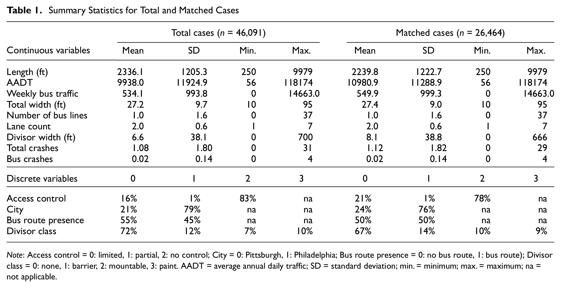
Note: Access control = 0: limited, 1: partial, 2: no control; City = 0: Pittsburgh, 1: Philadelphia; Bus route presence = 0: no bus route, 1: bus route); Divisor class = 0: none, 1: barrier, 2: mountable, 3: paint. AADT = average annual daily traffic; SD = standard deviation; min. = minimum; max. = maximum; na = not applicable.

Roadway geometry and traffic information for the segments was obtained for the statewide road network for each year from 2014 to 2017 through the Pennsylvania Spatial Data Access website. Although roadway geometry information did not change much across years, traffic exposure variables (e.g., AADT) changed every year. The analysis region was restricted to five counties in the city of Philadelphia: Philadelphia, Delaware, Chester, Montgomery and Bucks; and one county in Pittsburgh: Allegheny.

There is considerable variation in the operational schedules of bus lines. For instance, while some bus lines operate only on select days (e.g., weekdays or weekends), several others combine with other lines during off-peak hours or have varying bus routes for different times of the day. Therefore, average weekly bus traffic per segment was used as the measure of exposure for bus traffic as opposed to daily or specific time-of-day traffic counts. The operating schedules of bus services were obtained directly from the transit agencies. In Pittsburgh, 97 bus lines are operated by PAAC, and in Philadelphia, 124 routes are operated by SEPTA. Note that the study scope only includes bus services, therefore other transit modes operated by these agencies were not considered in the analyses. Because of the lack of historical data, bus schedules from 2018 were used in the study. Given that the study time period spanned 2014 to 2017, there was a mismatch between the schedule data and crash outcomes. Though this is an obvious limitation, we anticipated the bias from this disparity to be low given that we did not expect the average weekly transit patterns to have changed significantly over these years for a specific route.

However, to relax this assumption, the presence of a bus route was assigned only to those segments in which the historic presence of a bus route was evident, that is, from 2014 to 2016 for Philadelphia and for 2016 and 2017 for Pittsburgh. This assisted in maintaining continuity of the treatment application (i.e., the presence and intensity of a bus route). Furthermore, we contacted both transit agencies and confirmed that only minor changes were made during the study period; using the historical data available from PAAC we verified that the bus network had extended only 4.6% and only one route had been discontinued but its express option was still available in the physical route. SEPTA confirmed that no major changes were implemented during those dates.

Figure 1 shows the spatial distribution of bus traffic along the major arteries of the two cities. It can be seen that regions with a higher density of bus routes (e.g., downtown areas) are associated with higher bus traffic levels, which is consistent with the observations in the real world and with expectations.

Figure 1.

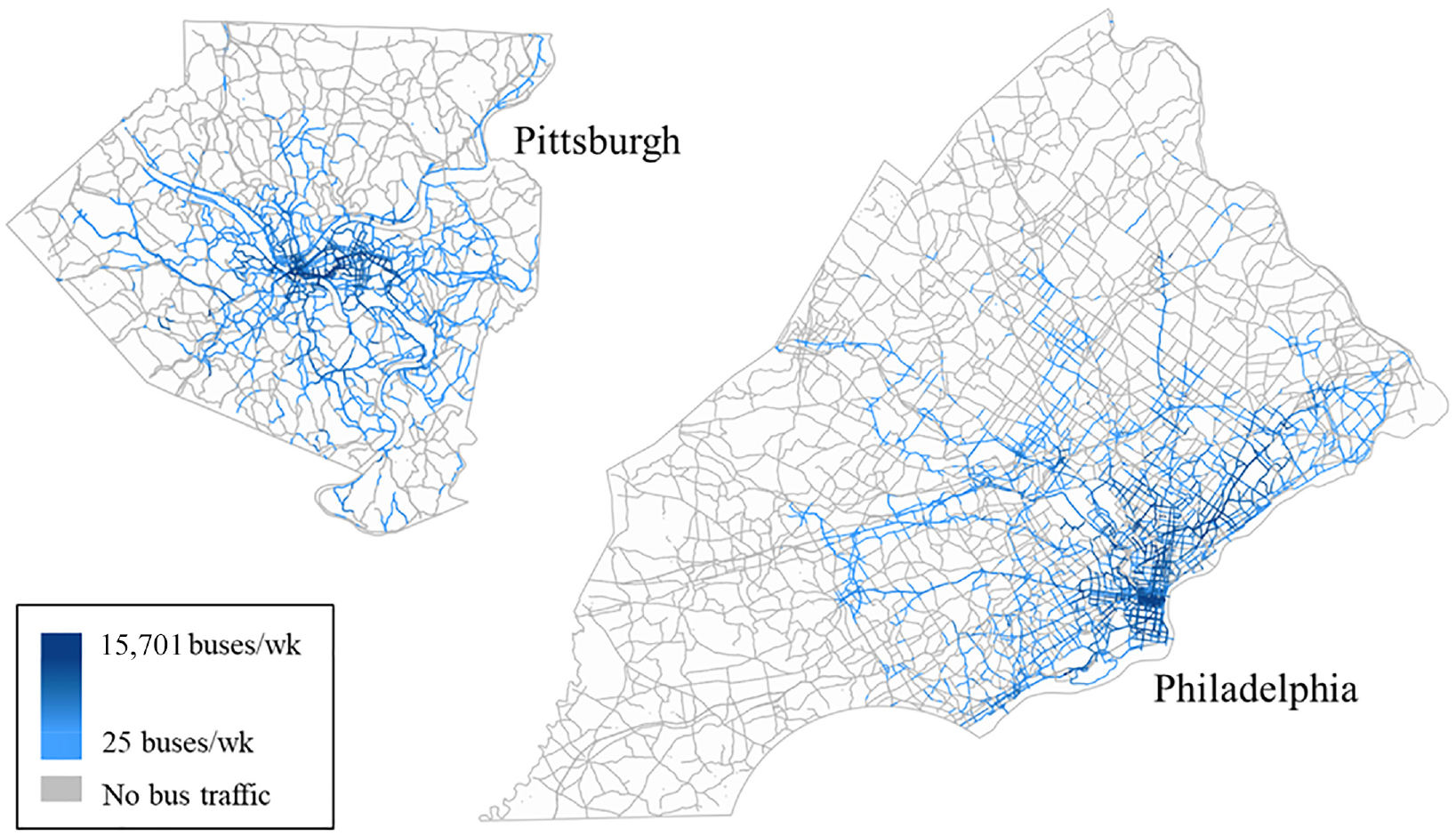
Weekly bus traffic for each segment in 2017.

Results

This section provides the results from the PS-PO matching process and the crash frequency estimation through SPF development.

Propensity Score Matching

The propensity score was determined through a logit model using the predictors presented in Table 2. The predictors used for this model fitting do not necessarily match those used for the development of the SPFs, since the scope of this stage was to compare segments by their infrastructure features and the presence of a bus route, regardless of the observed crash frequencies.

Table 2.

Summary Results of Propensity Score Estimation

Variable	Estimate	SE	P(>\|z\|)
(Intercept)	−1.562	0.159	8E-23
Natural log of segment length (feet)	−0.397	0.018	3E-102
Natural log of traffic volume (vehicles/day)	0.446	0.014	1E-230
Total width (feet)	0.107	0.002	0
Lane count	−1.120	0.027	0
Divisor class: paint (versus none)	1.337	0.039	3E-255
Divisor class: mountable (versus none)	0.314	0.043	2E-13
Divisor class: barrier (versus none)	0.488	0.039	8E-36
Access control: partial (versus limited)	−0.449	0.115	1E-04
Access control: no control (versus limited)	0.122	0.033	2E-04
City: Philadelphia (versus Pittsburgh)	−0.582	0.026	1E-109

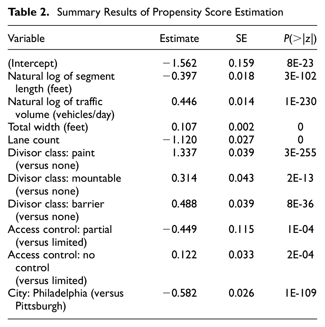
Figure 2 illustrates how the distributions of the propensity scores before the matching differ, being the control group (without a bus route) skewed to the right, while the treated group (with a bus route) has a bimodal profile. After the propensity score matching, both distributions had very similar shapes and scales, which is desirable for a balanced treatment evaluation. One disadvantage of the PS-PO method is that sample size is reduced because non-matched cases (43% of segments, in this case) are discarded. However, the matched sample consisted of 26,464 segments and was therefore still sufficient to produce reliable estimations.

Figure 2.

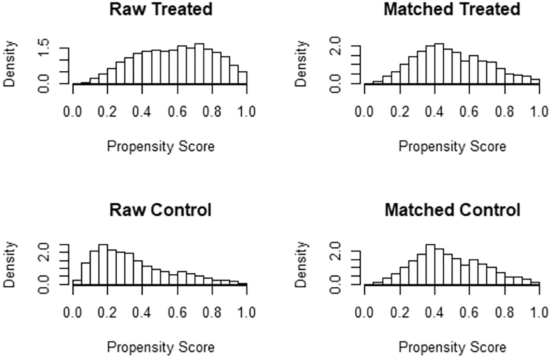
Histograms of propensity scores before and after the matching process.

The reduction in the standardized bias before and after implementation of the PS-PO is shown in Figure 3. It can be seen that all biases are less than 10% in absolute value compared with large bias values in the total (unmatched) sample. The PS-PO approach was successful in constructing comparable control and treatment group samples.

Figure 3.

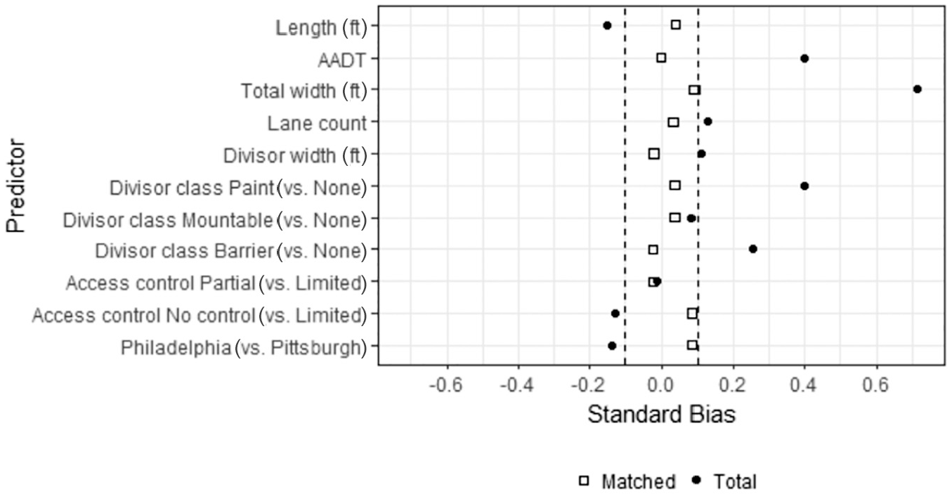
Standardized bias after the PS-PO implementation.

SPF Estimation for Total Crashes

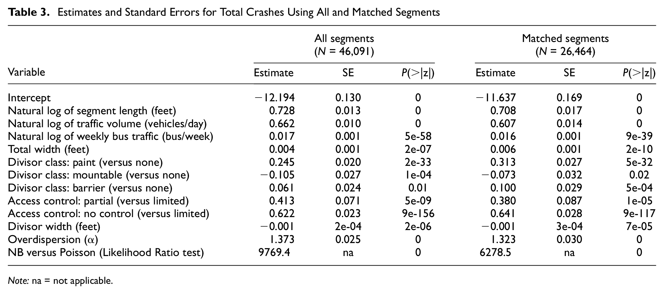
Crash frequency models were estimated using both matched and total data for comparison. The estimation results of these different models are shown in Table 3. Although the presence of a bus route and intensity of bus traffic were of interest in this research, both variables are highly correlated; therefore, average weekly bus traffic was used instead of the indicator variable for presence of bus lines to capture the impact of buses on crash occurrences in the final specification. In general, higher weekly bus traffic levels lead to higher expected crashes, even after controlling for regular traffic levels (AADT). Given the pseudo-causal inference from the properties of the PS-PO framework applied to the matched segments, the parameter estimate for weekly bus traffic suggests that there is an expected average increase of 0.016% crashes for every 1% increase in weekly bus traffic, which is a direct measure of pseudo-causal effect.

Table 3.

Estimates and Standard Errors for Total Crashes Using All and Matched Segments

Variable	All segments(N = 46,091)			Matched segments(N = 26,464)
Variable	Estimate	SE	P(>\|z\|)	Estimate	SE	P(>\|z\|)
Intercept	−12.194	0.130	0	−11.637	0.169	0
Natural log of segment length (feet)	0.728	0.013	0	0.708	0.017	0
Natural log of traffic volume (vehicles/day)	0.662	0.010	0	0.607	0.014	0
Natural log of weekly bus traffic (bus/week)	0.017	0.001	5e-58	0.016	0.001	9e-39
Total width (feet)	0.004	0.001	2e-07	0.006	0.001	2e-10
Divisor class: paint (versus none)	0.245	0.020	2e-33	0.313	0.027	5e-32
Divisor class: mountable (versus none)	−0.105	0.027	1e-04	−0.073	0.032	0.02
Divisor class: barrier (versus none)	0.061	0.024	0.01	0.100	0.029	5e-04
Access control: partial (versus limited)	0.413	0.071	5e-09	0.380	0.087	1e-05
Access control: no control (versus limited)	0.622	0.023	9e-156	0.641	0.028	9e-117
Divisor width (feet)	−0.001	2e-04	2e-06	−0.001	3e-04	7e-05
Overdispersion ( $α$ )	1.373	0.025	0	1.323	0.030	0
NB versus Poisson (Likelihood Ratio test)	9769.4	na	0	6278.5	na	0

Note: na = not applicable.

These results suggest that the presence and intensity of a bus services has a detrimental impact on safety for other road users. This finding is consistent with the model-free average impact of presence of bus routes on crash frequency, presented in the next subsection. The other roadway geometry variables in the model specification serve as control variables and can be interpreted in a straightforward way. For instance, roadway segments with partial access control or no access control had more crashes, on average, compared with segments with completely limited access control; i.e., the less control, the higher the expected crash frequency. This is expected given that controlled access reduces the number of traffic conflicts.

At first glance, there do not seem to be significant differences in the coefficient estimates between the models estimated for all segments and matched segments. However, when comparing both models closely, some differences stand out. For instance, between the unmatched and matched samples, the parameter estimates for total width, the divisor width, and for one of the indicator variables for divisor class (paint versus none) significantly increased their estimate, whereas the corresponding estimate on the indicator variable for the divisor class mountable (versus none) decreased by 43%. It is also important to note that the standard error estimates of parameters in the matched sample were higher than the corresponding values in the unmatched dataset. This is understandable given that standard error measures the degree of certainty in the mean parameter estimates and is inversely related to the sample size. However, the higher standard error in the matched sample did not affect the model inferences in this study given that the sample size was quite large (26,464 segments in the matched sample) as indicated by very low p-values. Furthermore, the statistically significant overdispersion parameter in the NB model underscored the importance of accounting for overdispersion in the crash data.

Another model that used an indicator variable for the presence of a bus route (as opposed to weekly bus traffic) was estimated to infer causal impact of bus routes on safety performance. This model had lower BIC and AIC values compared with the model with average weekly bus traffic reported in Table 3. We have not presented the results of this alternate model in the paper to conserve space. The relative magnitude and sign of all parameters in this model were the same as those shown in Table 3, but the indicator variable for the presence of a bus route had an estimate of 0.236 and a standard error of 0.014 (p-value significantly less than 0.001); therefore, the presence of a bus route was associated, on average, with a 27% $(e^{0.236} - 1)$ increase in the expected crash frequency of overall crashes, compared with segments where no bus route was present, which is a considerable effect.

Model-Free Analysis for Total Crashes

In addition to the model-based statistical inference implemented in the previous section, a model-free analysis was also undertaken. This was intended as a non-parametric analysis to evaluate the average change between treated and untreated segments. The average effect was also calculated for the entire population as well as within different sub-groups of roadway segments. For each categorical variable, this treatment difference $(T_{diff})$ was calculated as indicated in Equation 7:

T_{diff} = \frac{{\hat{y}}_{T} - {\hat{y}}_{UT}}{{SE}_{p}}

(7)

where

${\hat{y}}_{T}$ = the estimated mean of observed crashes from the treated sample (presence of a bus route in the segment),

${\hat{y}}_{UT}$ = is the estimated mean of observed crashes from the untreated sample, and

$S E_{p}$ = the pooled standard error from both samples.

This was calculated as shown in Equation 8.

\begin{matrix} S E_{p} = S_{p} \sqrt{\frac{1}{n_{T}} + \frac{1}{n_{UT}}} \\ = \sqrt{\frac{(n_{T} - 1) S_{T}^{2} + (n_{UT} - 1) S_{UT}^{2}}{n_{T} + n_{UT} - 2}} \sqrt{\frac{1}{n_{T}} + \frac{1}{n_{UT}}} \end{matrix}

(8)

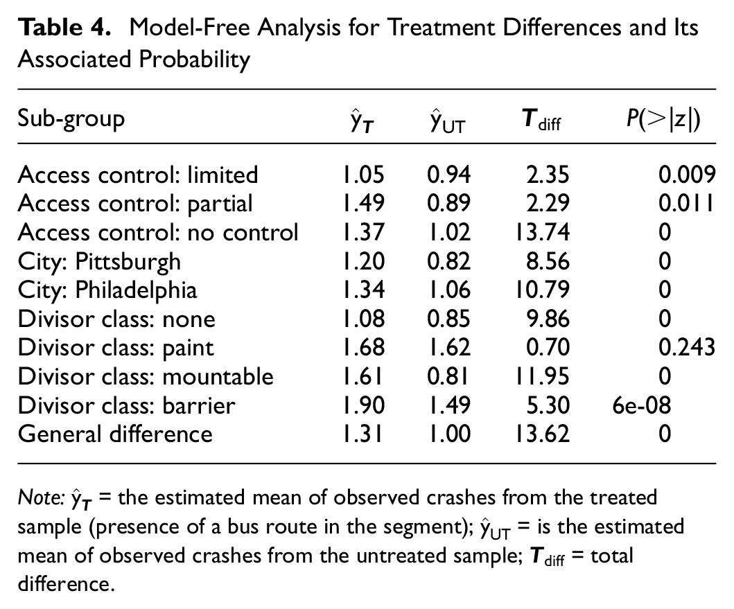
This procedure was repeated for each level of the categorical predictors and the results are presented in Table 4. Although the model-free approach can be seen as a non-parametric method, a normal probability was reported based on the large sample sizes and supported by the central limit theorem (minimum sample of 117 for any combination of treatment and category of a variable).

Table 4.

Model-Free Analysis for Treatment Differences and Its Associated Probability

Sub-group	${\hat{y}}_{T}$	${\hat{y}}_{UT}$	$T_{diff}$	P(>\|z\|)
Access control: limited	1.05	0.94	2.35	0.009
Access control: partial	1.49	0.89	2.29	0.011
Access control: no control	1.37	1.02	13.74	0
City: Pittsburgh	1.20	0.82	8.56	0
City: Philadelphia	1.34	1.06	10.79	0
Divisor class: none	1.08	0.85	9.86	0
Divisor class: paint	1.68	1.62	0.70	0.243
Divisor class: mountable	1.61	0.81	11.95	0
Divisor class: barrier	1.90	1.49	5.30	6e-08
General difference	1.31	1.00	13.62	0

Note: ${\hat{y}}_{T}$ = the estimated mean of observed crashes from the treated sample (presence of a bus route in the segment); ${\hat{y}}_{UT}$ = is the estimated mean of observed crashes from the untreated sample; $T_{diff}$ = total difference.

In the entire population of roadway segments, the model-free estimate of the average crash frequency on segments with a bus route was 1.31 compared with 1.00 for segments without it, that is, on average, the effect of the presence of at least one bus route led to 31% more crashes along roadway segments. For all sub-groups of roadway segments, the probability of the difference for the treatment being different than zero was less than the threshold of 0.05 and therefore considered statistically significant. Only for the sub-group of segments that had painted dividers was the effect not statistically significant. Moreover, all differences were positive, meaning that the observed crash frequencies for segments with a bus route were higher than for segments without, which is consistent with the findings from the NB approach presented previously.

Model for Crashes Involving Buses

The earlier part of this study focused on estimating the impact of the presence of a bus route and the intensity of bus traffic on overall crash frequency, which is of great interest to transportation safety agencies. In addition, the frequency of crashes involving buses and associated factors are of particular interest to transit agencies given that this has a direct impact on their day-to-day operations. Therefore, in addition to the models that focused on all types of crashes, supplementary models that focused exclusively on bus-related crashes were developed, that is, crashes that involved at least one non-school bus and occurred on a bus route of services provided by either PAAC or SEPTA. By this definition, only the segments with at least one bus route were used for this subsection.

The results presented in Table 5 show that higher levels of both overall traffic volume (AADT) and average weekly bus traffic are associated with more bus crashes. However, the marginal impact of weekly bus traffic is higher than the marginal impact of AADT, which was expected, but had not been yet quantified. Higher roadway width and access control (the less limited, the more crashes expected) were associated with higher bus crash frequencies. Note that the divisor class (none, paint, mountable, or barrier) is no longer significant in this model.

Table 5.

Estimates and Standard Errors for Bus Crashes Using All Segments Where Bus Routes are Present

Variable	All segments (n = 20,857)
Variable	Estimate	SE	P(>\|z\|)
(Intercept)	−20.562	0.981	2e-97
Natural log of segment length (feet)	0.620	0.075	1e-16
Natural log of traffic volume (vehicles/day)	0.353	0.068	2e-07
Natural log of weekly bus traffic (bus/week)	1.032	0.051	3e-90
Total width (feet)	0.012	0.003	4e-04
Access control: partial (versus limited)	0.933	0.629	0.138
Access control: no control (versus limited)	1.626	0.212	2e-14
Overdispersion ( $α$ )	0.551	0.100	2e-08
NB versus Poisson (Likelihood Ratio test)	67.3	na	2e-16

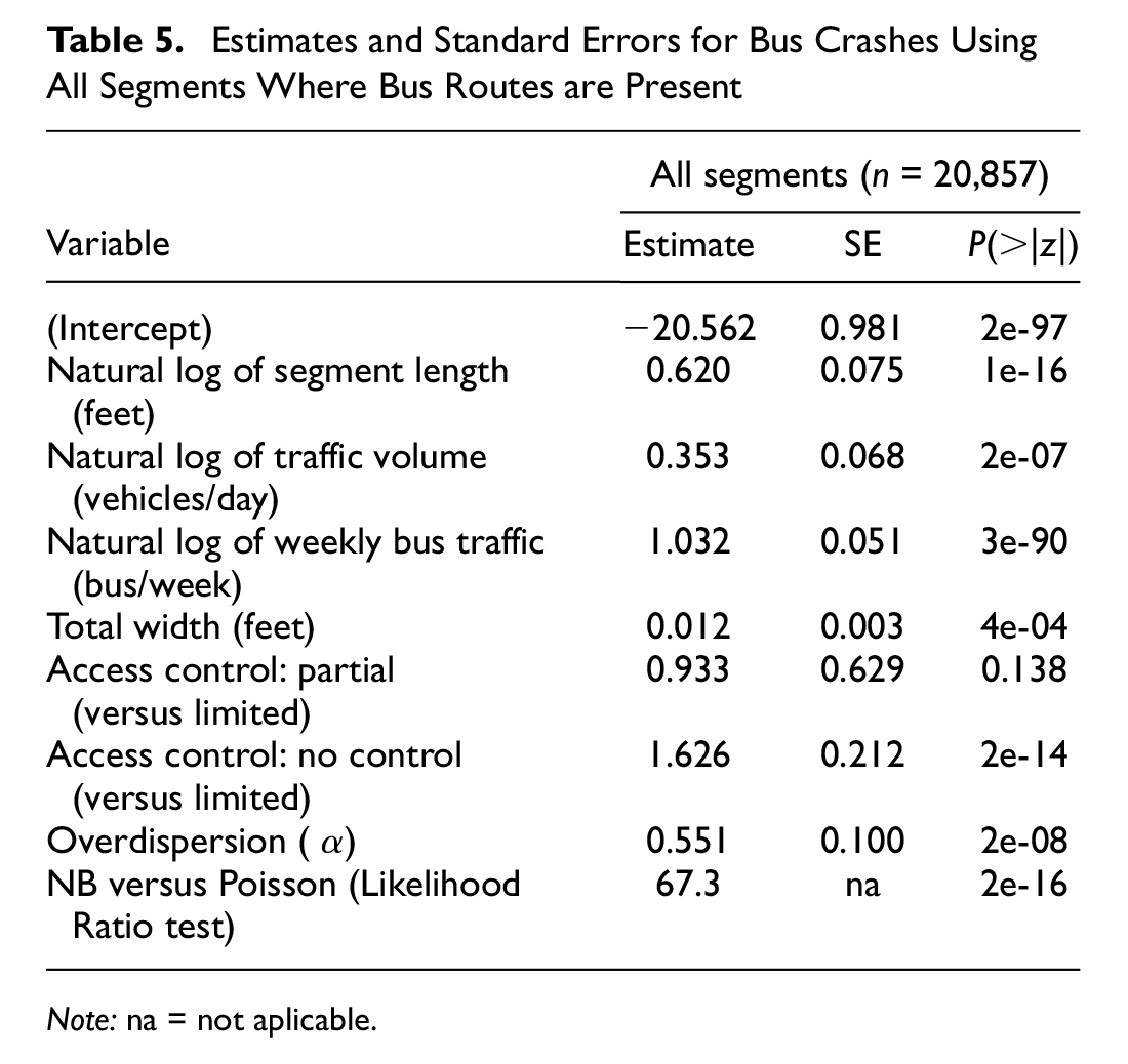
Note: na = not aplicable.

Discussion and Concluding Remarks

Mixed traffic conditions with passenger cars and heavy vehicles tend to be riskier for travelers compared with homogenous traffic conditions. However, the causal impact of mixed bus and general traffic on traffic safety has not been adequately captured in the safety literature. In this paper, the pseudo-causal impact of bus routes on crashes was captured using a combination of the PS-PO framework and crash frequency models. The results indicate that the presence of bus routes along roadway segments increased the average crash frequency by about 27% per year, compared with segments with no bus route presence. Moreover, a 1% increase in average weekly bus traffic resulted in 0.017% more crashes per year.

Although this study demonstrated a pseudo-causal relationship between bus lines and crashes, more research is needed to understand the nature of these crashes. For instance, given that buses in urban roads are associated with lower speeds, it is possible that bus lines lead to a reduction in severe crashes but an increase in property-damage crashes. Furthermore, this study assumed that there were no omitted variables that affected both treatment (i.e., the presence of bus lines) and outcomes (i.e., crash frequency). These omitted variables can confound the impact of bus routes and lead to over-estimation of the causal effects. For example, land use in the proximity of roadway segments can affect crash occurrences as well as provision of bus services leading to confounding effects. Future studies must attempt to include these confounding variables or use alternate causal inference methods such as the instrument variable method.

To avoid misinterpretation of the results from this study, we would like to clarify that the results of this study do not suggest that bus routes should be removed to decrease crash frequencies. Instead, they indicate that there are safety issues that need to be studied in greater detail along with possible countermeasures. There are multiple reasons for which transit is necessary, and these reasons include road safety benefits. For instance, consider a case in which all bus routes were eliminated and all passengers switched to private vehicles.

Assuming an average car occupancy of 1.5 passengers (pax)/vehicle ( 31 ) and an average daily bus ridership of 49.1 pax/bus for SEPTA and 29.5 pax/bus for PAAC (according to their operation and financial releases for 2019), and knowing that 79% of the road segments in this study are located in Philadelphia, the weighted average daily bus ridership is

49.1 \frac{pax}{bus} * 79 % + 29.5 \frac{pax}{bus} * 21 % = 44.8 \frac{pax}{bus}

(9)

The average bus traffic by segment from Table 1 is $549.9$ buses per week, meaning the additional AADT when removing a bus route is

549.9 \frac{bus}{week} * 44.8 \frac{pax}{bus} \div 1.5 \frac{pax}{car} \div \frac{7 days}{week} = 2345.9 \frac{car}{day}

(10)

The change in crash frequency when a bus route is removed from a given segment is

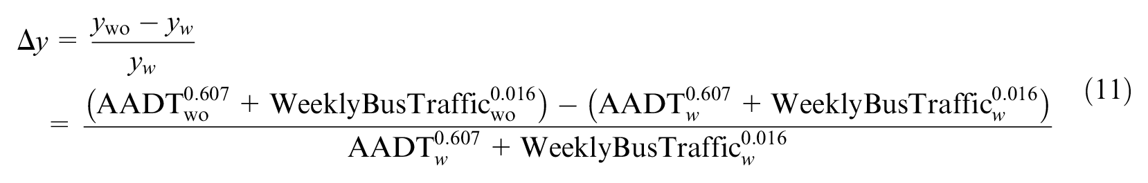
\begin{matrix} Δ y = \frac{y_{wo} - y_{w}}{y_{w}} \\ = \frac{({AADT}_{wo}^{0.607} + {WeeklyBusTraffic}_{wo}^{0.016}) - ({AADT}_{w}^{0.607} + {WeeklyBusTraffic}_{w}^{0.016})}{{AADT}_{w}^{0.607} + {WeeklyBusTraffic}_{w}^{0.016}} \end{matrix}

(11)

where the subscript wo refers to a segment without bus routes and w refers to segments with bus routes, and the values correspond to the estimated coefficients from Table 3 for the matched cases. Using the average values presented in Table 1, the average percent change in crash frequency when removing bus routes from a segment is

\frac{y_{w o} - y_{w}}{y_{w}} = \frac{({(10980.9 + 2345.9)}^{0.607} + 0^{0.016}) - ({10980.9}^{0.607} + {549.9}^{0.016})}{{10980.9}^{0.607} + {549.9}^{0.016}} = 12.1 %

(12)

This implies a direct increase of 12.1% in crash frequency if people that currently use the bus service started using only private vehicles, which, although extreme, seems reasonable since bus services are motorized means of transportation that are unlikely to be replaced by active mobility given the long distances traveled. Therefore, removing bus routes would only increase the crash frequency; we therefore emphasize the need to explore this topic in more detail rather than considering removing bus routes as a possible alternative.

Footnotes

Author Contributions

The authors confirm contribution to the paper as follows: study conception and design: R. Guadamuz, V. Gayah, R. Paleti; analysis and interpretation of results: R. Guadamuz, V. Gayah, R. Paleti; draft manuscript preparation: R. Guadamuz, V. Gayah, R. Paleti. All authors reviewed the results and approved the final version of the manuscript.

Declaration of Conflicting Interests

The author(s) declared no potential conflicts of interest with respect to the research, authorship, and/or publication of this article.

Funding

The author(s) received no financial support for the research, authorship, and/or publication of this article.

References

American Association of State Highway and Transportation Officials (AASHTO). The Highway Safety Manual. Washington, D.C., 2010.

Lord

Mannering

The Statistical Analysis of Crash-frequency Data: A Review and Assessment of Methodological Alternatives. Transportation Research Part A: Policy and Practice, Vol. 44, No. 5, 2010, pp. 291–305.

Duduta

Adriazola

Hidalgo

Lindau

L. A.

Jaffe

Understanding Road Safety Impact of High-performance Bus Rapid Transit and Busway Design Features. Transportation Research Record: Journal of the Transportation Research Board, 2012. 2317: 8–14.

Pecheux

Saporta

Light Rail Vehicle Collisions with Vehicles at Signalized Intersections (Vol. 79). Transportation Research Board, Washington, D.C., 2009.

Duduta

Adriazola

Hidalgo

Lindau

L. A.

Jaffe

Traffic Safety in Surface Public Transport Systems: A Synthesis of Research. Public Transport, Vol. 7, No. 2, 2014, pp. 121–137.

Bocarejo

Velasquez

Díaz

Tafur

Impact of Bus Rapid Transit Systems on Road Safety: Lessons from Bogotá, Colombia. Transportation Research Record: Journal of the Transportation Research Board, 2012. 2317: 1–7.

Goh

Currie

Sarvi

Logan

Road Safety Benefits from Bus Priority: An Empirical Study. Transportation Research Record: Journal of the Transportation Research Board, 2013. 2352: 41–49.

Dharmaratne

S. D.

Stevenson

Public Road Transport Crashes in a Low Income Country. Injury Prevention, Vol. 12, No. 6, 2006, pp. 417–420.

Goh

K. C. K.

Currie

Sarvi

Logan

Bus Accident Analysis of Routes with/without Bus Priority. Accident Analysis & Prevention, Vol. 65, 2014, pp. 18–27.

10.

Mallia

Lazuras

Violani

Lucidi

Crash Risk and Aberrant Driving Behaviors among Bus Drivers: The Role of Personality and Attitudes Towards Traffic Safety. Accident Analysis & Prevention, Vol. 79, 2015, pp. 145–151.

11.

Oluwole

A. M.

Development of Relationship Between Risk Factors and Road Safety Practices Among Bus Drivers Using Structural Model. Doctoral dissertation. Universiti Teknologi Malaysia, 2015.

12.

Anund

Ihlström

Fors

Kecklund

Filtness

Factors Associated with Self-Reported Driver Sleepiness and Incidents in City Bus Drivers. Industrial Health, Vol. 54, No. 4, 2016, pp. 337–346.

13.

Q. N.

Van Duong

Lee

A. H.

Meuleners

L. B.

Factors underlying bus-related crashes in Hanoi, Vietnam. Transportation Research Part F: Traffic Psychology and Behaviour, Vol. 46, 2017, pp. 426–437.

14.

Taylor

B. D.

Fink

C. N. Y.

Explaining Transit Ridership: What Has the Evidence Shown?

Transportation Letters, Vol. 5, No. 1, 2013, pp. 15–26.

15.

QGIS Development Team. QGIS Geographic Information System. Open Source Geospatial Foundation Project. 2019. http://qgis.osgeo.org

16.

ESRI. ArcGIS Desktop: Release 10.6. Environmental Systems Research Institute, Redlands, Calif., 2018.

17.

Gooch

Gayah

Donnell

Safety Performance Functions for Horizontal Curves and Tangents on Two-lane, Two Way Rural Roads. Accident Analysis & Prevention, Vol. 120, 2018, pp. 28–37.

18.

Donnell

Gayah

Regionalized Safety Performance Functions. Final Report for the Pennsylvania Department of Transportation, FHWA-PA-2016-001-PSU WO 17, 2016.

19.

Donnell

Gayah

Regionalized Urban-Suburban Collector Road Safety Performance Functions. Final Report for the Pennsylvania Department of Transportation, PA-2019-01-511601 WO 007, 2018.

20.

Holmes

W. M.

Using Propensity Scores in Quasi-experimental Designs. Thousand Oaks, SAGE Publications, 2013.

21.

Aul

Davis

Use of Propensity Score Matching Method and Hybrid Bayesian Method to Estimate Crash Modification Factors of Signal Installation. Transportation Research Record: Journal of the Transportation Research Board, 2006. 1950: 17–23. https://doi.org/10.3141/1950-03.

22.

Karwa

Slavkovi

A. B.

Donnell

E. T.

Causal Inference in Transportation Safety Studies: Comparison of Potential Outcomes and Causal Diagrams. The Annals of Applied Statistics, Vol. 5, No. 2B, 2011, pp. 1428–1455. https://doi.org/10.1214/10-AOAS440.

23.

Wood

J. S.

Porter

R. J.

Safety Impacts of Design Exceptions on Nonfreeway Segments. Transportation Research Record: Journal of the Transportation Research Board, Vol. 2358, 2013, pp. 29–37. https://doi.org/10.3141/2358-04.

24.

Sasidharan

Donnell

Propensity Scores-potential Outcomes Framework to Incorporate Severity Probabilities in the Highway Safety Manual Crash Prediction Algorithm. Accident Analysis & Prevention, Vol. 71, 2014, pp. 183–193.

25.

Wood

J. S.

Gooch

J. P.

Donnell

E. T.

Estimating the Safety Effects of Lane Widths on Urban Streets in Nebraska Using the Propensity Scores-potential Outcomes Framework. Accident Analysis & Prevention, Vol. 82, 2015, pp. 180–191.

26.

Gooch

Gayah

Donnell

Quantifying the Safety Effects of Horizontal Curves on Two-way, Two-lane Rural Roads. Accident Analysis & Prevention, Vol. 92, 2016, pp. 71–81.

27.

Hirano

Imbens

G. W.

Ridder

Efficient Estimation of Average Treatment Effects Using the Estimated Propensity Score. Econometrica, Vol. 71, No. 4, 2003, pp. 1161–1189.

28.

Harder

V. S.

Stuart

E. A.

Anthony

J. C.

Propensity Score Techniques and the Assessment of Measured Covariate Balance to Test Causal Associations in Psychological Research. Psychological Methods, Vol. 15, No. 3, 2010, p. 234.

29.

Austin

P. C.

An Introduction to Propensity Score Methods for Reducing the Effects of Confounding in Observational Studies. Multivariate Behavioral Research, Vol. 46, No. 3, 2011, pp. 399–424.

30.

Washington

S. P.

Karlaftis

M. G.

Mannering

Statistical and Econometric Methods for Transportation Data Analysis. Chapman and Hall/CRC, 2010.

31.

Boundy

R. G.

Transportation Energy Data Book: Edition 37 (No. ORNL/TM-2018/987). Oak Ridge National Lab.(ORNL), Oak Ridge, TN, 2019.