Exploring Artificial Neural Network to Evaluate the Undrained Shear Strength of Soil from Cone Penetration Test Data

Abstract

In geotechnical design practices, the undrained shear strength of soil is regarded as one of the engineering properties of paramount importance. Over the past years, several theoretical and empirical methods have been developed to estimate the undrained shear strength based on soil properties using in-situ tests such as cone and piezocone penetration tests (CPT and PCPT). However, most of these methods involve correlation assumptions that can result in inconsistent accuracy. In this paper, an artificial neural network (ANN) is used to devise a model with a better and more consistent prediction of the undrained shear strength of soil from CPT data. The ANN algorithm does not require such assumptions as it learns from previous cases/instances. A database was prepared of soil boring data and laboratory test data along with corresponding CPT/PCPT data from 70 test sites located in 14 different parishes in Louisiana. Presenting this data to the ANN, models were trained through trial and error using different network algorithms, such as back propagation method and quasi-Newton method. Different ANN models were trained using corrected cone tip resistance and sleeve friction input data along with some other easily measurable soil properties. The results of ANN models were then compared with a conventional empirical method of determining undrained shear strength of soil from CPT parameters. The results of this study clearly demonstrated that the ANN models outperformed the conventional empirical method, which confirms the applicability of ANN in the evaluation of the undrained shear strength of soil from CPT data.

The undrained shear strength of soil refers to the capability of soil to withstand shear stress. It is one of the prime parameters in the calculation of many geotechnical engineering phenomena, for instance, settlement. In the design of foundations (both shallow and deep foundations), the undrained shear strength of soil is also of paramount importance. Therefore, scrupulous evaluation of the shear strength of soil is imperative. Over the years, researchers had developed numerous analytical and empirical methods to determine the shear strength of soil, for example, bearing capacity (BCM), strain path (SPM), cavity expansion (CEM), and finite element (FEM) methods ( 1 ). Combinations of these methods have also been explored to gain a better interpretation of shear strength of soil, for example, CEM-FEM ( 2 ), CEM-SPM ( 3 ), CEM-BCM ( 4 ), and SPM-FEM ( 5 ). However, most of these methods incorporated simplifying assumptions regarding soil condition, boundary conditions, and soil failure criteria. Therefore, the findings of theoretical methods need verification from in-situ and laboratory soil parameters. The unconsolidated undrained triaxial test can be useful in this regard. Unfortunately, conducting triaxial tests is time consuming and expensive. Moreover, inevitable disturbance during collection, transportation, and handling of soil samples means that the test results are contentious to some extent.

In-situ cone penetration tests (CPT) and piezocone penetration tests (PCPT) can be effectively utilized for soil identification, evaluation of soil properties like shear strength of soil, and many other geotechnical applications. CPT is fast, reliable, and economical (savings up to around 70%) compared with the traditional soil characterization tests that involve soil boring and laboratory tests. This test can provide continuous data profiles with depth (i.e., cone tip resistance, cone sleeve friction, and porewater pressure) related to soil strength and stiffness parameters, which can be useful for estimation of undrained shear strength of soil. Therefore, several empirical methods were developed in recent decades to estimate the undrained shear strength from CPT parameters, by Lunne and Kleven ( 6 ), Senneset ( 7 ), and so forth. However, most of these methods involve several assumptions and judgments in selecting proper correlation coefficients such as, the cone tip factor, N_kt, between the CPT data profiles and undrained shear strength which can influence the calculation of shear strength. This can result in inconsistent accuracy of estimating the undrained shear strength for different site conditions.

In recent years, the artificial neural network (ANN) has emerged and been successfully implemented for different geotechnical engineering problems, such as settlement of shallow foundations, liquefaction potential, swelling pressure of expansive soil, load settlement behavior of pile foundations, and so forth. ( 8 – 15 ). The application of the ANN technique for estimating the undrained shear strength of soil from CPT parameters is expected to resolve the aforementioned shortcomings in traditional empirical methods, as it does not need any correlation assumption or judgment. Rather, the ANN technique, which represents a form of artificial intelligence, intends to replicate the way the human brain learns from previous cases/instances and is trained by using special mathematical algorithms. The ANN attempts to grasp the relationship between the input parameters: corrected cone tip resistance, cone sleeve friction, overburden pressure, and so forth. and the output parameter, the undrained shear strength of soil, using the set of available data collected from different project sites with different soil conditions. This can be achieved through repetitive training steps by adjusting the connection weights, number of nodes, and number of layers after each iteration. This involves forward prediction and backward corrections of the connection weights. The complexity of the ANN model can also be altered by changing the transfer function or the structure of the model ( 8 ). Once the most accurate ANN model is identified (i.e., number of layers and number of nodes per layer) after being well trained, the model can be applied for estimating the undrained shear strength of soil for new construction sites.

Objectives

The prime objective of this research study is to explore the applicability of using ANN in the prediction of undrained shear strength of soil from CPT data, generating a model that can be used in practical applications. The relative importance of different input parameters (e.g., cone tip resistance, cone sleeve friction, overburden pressure, etc.) in the estimation of undrained shear strength of soil will also be investigated. In addition, the ANN results will be compared with results of a verified data set of shear strength of soil from laboratory tests, as well as the results of the conventional method, to demonstrate ANN’s accuracy and confirm its reliability and feasibility.

Overview of ANN

The learning system of the human brain, which is composed of very complex webs of interconnected neurons, is the primary inspiration toward the development of ANNs. These are the modeling of the human brain with the simplest definition, in which the building blocks or nodes resemble the brain neurons ( 16 ). ANNs intend to replicate the way of the learning of human brain through certain mathematical algorithms. With the constitution of many neurons or simple processors, ANNs can perform parallel computation for complex and massive data processing and knowledge representation ( 16 ). The primary element of the ANN is the neurons, which are also called nodes or processing elements. These processing elements are generally arranged in several layers consisting of an input layer, one or a few intermediate layers and an output layer (Figure 1). The intermediate layers are also called hidden layers, as they do not interact directly with the external environment. Each layer consists of several neurons or nodes. The network is arranged in such a way that the output of one layer serves as the input for the following layer.

Figure 1.

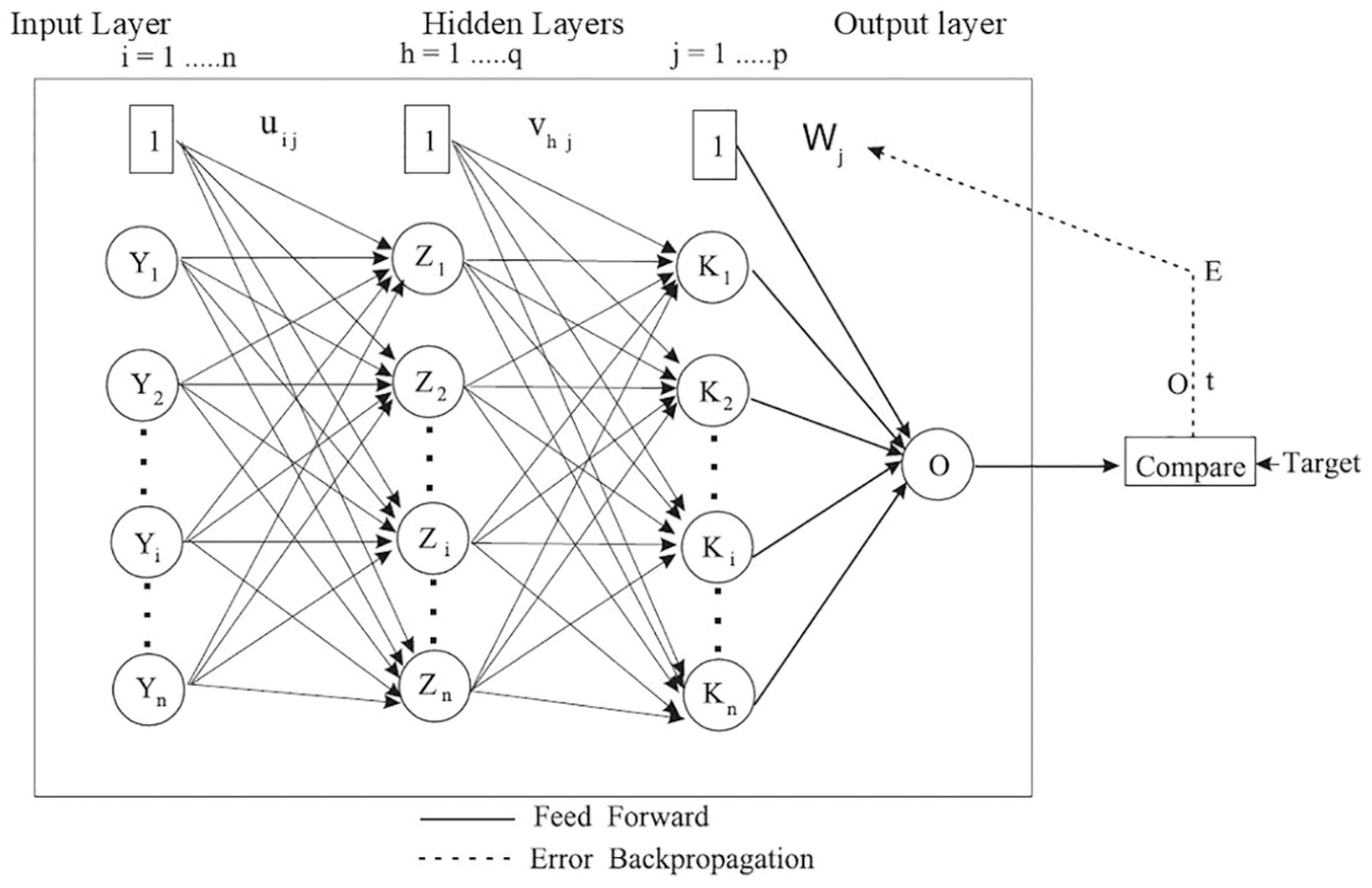
Typical structure of artificial neural network (ANN) ( 9 ).

The processing element of each layer is connected to other processing elements through weighted connections. Between the interconnected neurons, corresponding weights are the determinant of the strength of the connections. No connection between two neurons is signified with a zero weight, whereas a negative weight refers to a repressive relation. An individual processing node receives weighted inputs, which are then summed and added with a bias factor, for the purpose of scaling the input parameters to certain range so that the convergence properties of the ANN are improved (added or subtracted). The result is then propagated through a transfer function (e.g., step, linear, ramp, logistic sigmoid, or hyperbolic tangent) to generate the output of the neuron. For any node j in layer l, the above stated process can be summarized in Equations 1 and 2 as follows ( 12 ):

{I_{j}}^{l} = θ_{j}^{l} + \sum_{n = 1}^{i} w_{ji}^{l} x_{i}^{l - 1}

(1)

{y_{j}}^{l} = f (I_{j})

(2)

where I_j^l = activation level of node j; $w_{ji}^{l}$ = connection weight between nodes i and j; $x_{i}^{l - 1}$ = input from node i; i = 0, 1, …, n; $θ_{j}^{l}$ = w_j0= bias for node j; y_j^l = output of node j; and f(I_j) = transfer function. The hyperbolic tangent function (tanh) was used in this study, which is the hyperbolic analog of the tan circular function. It is one of the most used functions for neural networks where the output ranges between –1 and +1. Ideally, tanh (I_j) = ( $e^{I_{j}} - e^{- I_{j}}$ ) / ( $e^{I_{j}} + e^{- I_{j}}$ ). The network is then propagated forward leading to final output, y_j. It is then compared with the target output, y_t and error, E, of the network is then calculated as, E = ½ $\sum (y_{t} - y_{j})$ ².

The backpropagation algorithm used in this study is a well-known procedure for training supervised networks ( 17 ). The backpropagation algorithm can be summarized as follows ( 18 ),

The input vector x can be labeled as x₁⁰,x₁⁰,x₃⁰….x_m^o.

The connection weights can be then assigned as w_ji^l where l=0,1,2….l.

The network will then be propagated forward using Equations 1 and 2

{I_{j}}^{l} = θ_{j}^{l} + \sum_{n = 1}^{i} w_{ji}^{l} x_{i}^{l - 1}

{y_{j}}^{l} = f (I_{j})

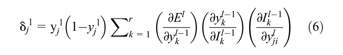
Then correction factor δ, for each neuron j in output layer (l=l) can be calculated from:

{δ_{j}}^{l} = (y_{t} - {y_{j}}^{l}) {y_{j}}^{l} (1 - {y_{j}}^{l})

(3)

Then w_ji^l needs to be updated using the following,

Δ {w_{ji}}^{l (current)} = η {δ_{j}}^{l} x_{l}^{1} + μ Δ {w_{ji}}^{l (previous)}

(4)

Equation 4 is a modified version of the delta rule ( $Δ$ w_ji^l = ηδ_j^lx_l^l–1) that contains the momentum rate, µ (0< µ < 1). This equation is also called the generalized delta rule with momentum term ( 17 ). By allowing a portion of previous updating (magnitude and direction) to be added to the current update value, the momentum is included to direct the search toward global minimum. The bias can be updated as,

Δ θ_{ji}^{l (current)} = η {δ_{j}}^{l} + μ Δ {θ_{ji}}^{l (previous)}

(5)

Similarly, for hidden layers,

{δ_{j}}^{l} = {y_{j}}^{l} (1 - {y_{j}}^{l}) \sum_{k = 1}^{r} (\frac{\partial E^{l}}{\partial y_{k}^{l - 1}}) (\frac{\partial y_{k}^{l - 1}}{\partial I_{k}^{l - 1}}) (\frac{\partial I_{k}^{l - 1}}{\partial y_{ji}^{l}})

(6)

Weights and biases will be updated using Equations 4 and 5 respectively.

Steps 1–7 are repeated until outputs are within a certain tolerance.

CPT and Borelog Database

In this research work, laboratory tests on soil samples (water content, unit weight, Atterberg limits, etc.) were performed as well as in-situ CPT/PCPT testing at a total of 70 test sites located in 14 different parishes in Louisiana. Figure 2 portrays the locations of the test sites. The laboratory test program comprised undisturbed Shelby tube samples from different depths of the bore hole of each site. Water content, grain size distribution, Atterberg limits, and specific gravity tests were performed as described by ASTM standards D 4643, D 7263, D 422, D 4318, and D 422 respectively. Furthermore, to evaluate the undrained shear strength of the soil, triaxial unconsolidated undrained tests were performed in compliance with the ASTM standard D 2850-03a.

Figure 2.

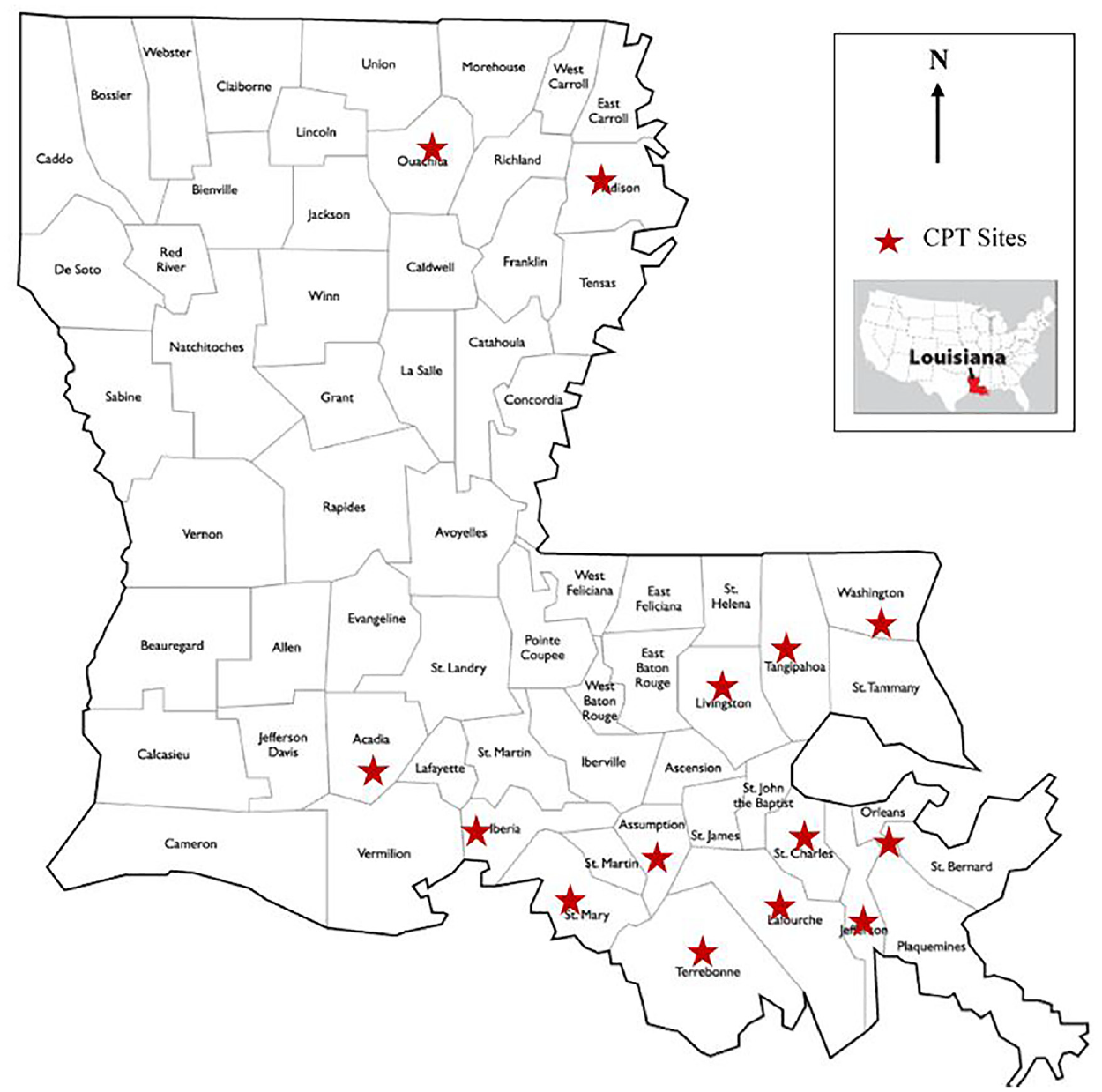
Locations of cone penetration test (CPT) sites

The in-situ test principally involved CPT or PCPT performed around the drilled boreholes, using 1.55 in.² (10 cm²) and 2.33 in.² (15 cm²) piezocone penetrometers. The CPT provided measured cone tip resistance, q_c, and cone sleeve friction, f_s, while the PCPT assessed the same with the inclusion of excess pore pressure behind the cone, u₂. The cone was pushed at a constant penetration rate of 0.79 in./sec (2 cm/sec) and the data were collected at constant intervals of 2 cm along the depth. PCPT was performed at 11 sites CPT at remainder of the sites.

Development of ANN

Development of an ANN model calls for several parameters such as model inputs and outputs, data division and pre-processing of available data, proper network architecture, training or optimization of connection weights, stopping criteria, and validation ( 8 ). Data from CPT/PCPT testing at 70 sites along with the laboratory test data was used in this study to train (calibrate), test (verify), and validate the neural network model(s). The personal computer-based software Neural Designer, developed by Artificial Intelligence Techniques Ltd. (https://www.neuraldesigner.com), was used in this work to simulate the ANN models.

Model Inputs and Outputs

In the development of ANN models, selection of the model input variables is very important as it has the most significant impact on model performance. Quality selection of input variables can improve the model performance to a great extent. A large number of input variables usually increases network size resulting in a decrease in processing speed. Consequently, the efficiency of the network is reduced. In this work, different combinations of input variables were used to train a number of neural networks to find the network that generates the best results. Based on prior knowledge from the literature, the chosen input variables were: corrected cone tip resistance, q_t, cone skin friction, f_s, overburden pressure, σ_vo, liquid limit, LL, and plastic limit, PL. The undrained shear strength, S_u, of soil was the only output (ranging from 80 pounds per square foot [psf] to 5870 psf) that was obtained from unconsolidated undrained triaxial test of undisturbed samples. Undrained shear strength depends greatly on the soil properties. CPT is a very strong tool that has been used over the years to measure soil strength. Consequently, among the input parameters, CPT tip resistance, q_c, and CPT skin friction, f_s, are more significant in quantifying the soil characteristics. Therefore, correction was made for tip resistance as the generated excess pore water pressure behind the cone can affect the total stress measured by the cone tip. The corrected cone tip resistance, q_t, is defined as:

q_{t} = q_{c} + (1 - a) \times u_{2}

(7)

where a = a_n/a_c is the effective area ratio of the cone; a_n is the cross-sectional area of the load cell; a_c is the projected area of the cone; and u₂ is the porewater pressure behind the cone.

As the CPT/PCPT provides continuous data, the average of corrected cone tip resistance, q_t-avg, and the average of cone skin friction, f_s-avg, was used in this study. In detail, the average q_t value of total 3ft (Figure 3) of soil was calculated for each soil layer from where the undisturbed sample was collected. The average f_s value was collected similarly. For the relevant soil layer, the overburden pressure, σ_vo, was calculated up to point A (Figure 3). For this specific soil layer, other necessary parameters (e.g., LL, PL, S_u, etc.) were determined from laboratory tests.

Figure 3.

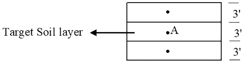
Data points selection system.

After the compilation of the database, input variables were used in different combinations to find the optimal ANN model that yields the best prediction in the evaluation of undrained shear strength. Six different types of ANN model input patterns (Table 1) were used in this research work. Based on prior research works from the literature, q_t-avg was considered in all the types of ANN models. In conjunction with q_t-avg, the rest of the input variables were tried in different combinations. Both direct (only CPT parameters) and indirect (CPT parameters along with a few easily attainable soil properties) approaches were considered in this study to evaluate S_u from CPT parameters.

Table 1.

Artificial Neural Network (ANN) Model Types Used in This Research

ANN model type	Parameters used as inputs
Type 1	(1) q_t-avg, (2) f_s-avg
Type 2	(1) q_t-avg, (2) f_s-avg, (3) σ_vo
Type 3	(1) q_t-avg, (2) σ_vo
Type 4	(1) q_t-avg–σ_vo
Type 5	(1) q_t-avg–σ_vo, (2) f_s-avg, (3) LL, (4) PL
Type 6	(1) q_t-avg, (2) f_s-avg, (3) σ_vo, (4) LL, (5) PL

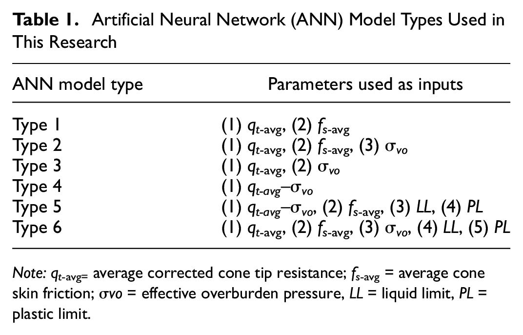
Note: q _t-avg ₌ average corrected cone tip resistance; f_s-avg = average cone skin friction; σvo = effective overburden pressure, LL = liquid limit, PL = plastic limit.

Data Division and Pre-Processing

The input data set is usually split into two subsets: a training set and an independent validation set. The training set is used to build the ANN model while the validation set is kept for validating the model’s performance. Hammerstrom ( 19 ) suggested using two-thirds of the database for model training and the remaining one-third for validation. Stone ( 20 ) introduced a cross-validation method which indeed is a modification of the data division method. This technique requires the data set to be divided into three sub sets, namely, training, testing and validation. The training set is used to improve the connection weights, while the testing set tests the performance of the model at different stages of training to determine when to stop the training process so that overfitting does not occur. The function of the validation set is to determine the performance of the trained network. Shahin et al. ( 21 ) concluded that there is no distinct relationship between the proportion of data among the subsets and the model performance. However, they obtained the best result using a combination of 20% of the data for validation and 80% of the data for network modeling (of which, 70% for training and 30% for testing). Another study used 65% of the primary database for training, 25% for testing, and 10% for validation ( 22 ). In this research work, the data from the 70 sites in Louisiana were divided as 70% for training, 15% for testing, and 15% for validation.

In the majority of the applications of ANN in geotechnical engineering, the data are randomly divided into their subsets. Since the ANN models have difficulty in extrapolating beyond the range of the training data ( 23 ), all the existing patterns available in the data set need to be included in the training set to develop a good ANN model. If the highest or extreme data points are excluded from the training data set, validation data will test the model’s extrapolation capability instead of its interpolation ability. Consequently, the model will not perform effectively. Therefore, care was taken to avoid this scenario.

After the available data from the 70 sites has been divided into corresponding subsets (i.e., training, testing, and validation), it is necessary to pre-process the data in a congenial form prior to their application to the ANN. This ensures all variables receive equal importance during the training. In addition, processing the data prior to training can sometimes aid in accelerating the convergence. Several techniques are available to be used to pre-process data such as data transformation, reducing input dimensionality, and noise removal. Normalization or scaling of data before application is also useful to prevent larger numbers from quashing smaller ones. However, scaling may not be necessary if all the data are of the same order of magnitude, which is not likely to be the case in the data set of this study. Therefore, the data in this study were scaled within the data limits.

ANN Network Architecture

In developing ANN models, determination of the network architecture is an important and difficult task at the same time. This involves the selection of the optimum number of layers and the number of nodes in each layer. It is generally done by choosing the number of layers first and then fixing the number of nodes in corresponding layers. However, there are always two layers in any neural network to represent the input and output variables. Therefore, the choice of number of hidden layers is the crucial step. It has been shown in the literature that a single hidden layer is enough most of the time to approximate any continuous function with sufficient connection ( 24 , 25 ). However, some researchers ( 23 , 26 ) have suggested the use of more than one hidden layer to provide the flexibility needed for modeling complex functions in many situations. In this regard, it is also found in the literature ( 27 ) that two hidden layers are enough. Extraction of the local features of the input patterns is accomplished in the first hidden layer, while the second hidden layer extracts the global features of the training patterns ( 28 ). However, more than one hidden layer often slows the training process down. Consequently, the chance of getting trapped in local minima increases ( 29 ).

The number of nodes in the input and output layers is usually determined by the number of model input and output parameters respectively. There is hardly any explicit approach to quantify the optimum number of nodes in a certain hidden layer. A trial-and-error procedure is usually conducted to estimate the number of nodes in each hidden layer. While doing so, it is important to remember that neural networks comprised of large numbers of hidden layer nodes are susceptible to overfitting and poor generalization ( 16 ). To obtain satisfactory performance of the model, therefore, the number of hidden nodes should be kept to a minimum. This will lead to: (a) reduction of computational time required for the training stage; (b) better generalization performance; (c) less vulnerability to the problem of overfitting; and (d) comparatively easier analysis of the trained network ( 30 ). Initially, the number of hidden nodes can be considered at 75% of the number of input units ( 31 ). Also, a number between the average and the sum of the nodes in both input and output layers can be considered as the number of hidden nodes ( 32 ). In this case, the highest allowable number of hidden nodes in a single layer network can be considered as (2I+1), where I is the number of inputs ( 33 ). However, it is better to start with a small number of nodes and then gradually increase the number until no significant improvement in the performance of the model is obtained ( 34 ). For networks with two hidden layers, the geometric pyramid rule ( 34 ) can be used, where the number of nodes in each layer decreases from the input layer toward the output layer.

Considering all the facts, starting from one, up to three hidden layers with different combinations of nodes were explored in this study. For a single hidden layer, the maximum number of nodes was 2I+1 while for double and triple hidden layers the geometric pyramid rule was followed. The input layer consisted of nodes varying in number from one to five, depending on the ANN type. However, for all the ANN types, the number of nodes in the output layer was only one, the undrained shear strength, S_u.

Training of ANN Models

Training of ANN models refers to the process of initializing a network through the deployment of initial values and then optimizing the connection weights to obtain global minima instead of a local one. A very widely used method to obtain the optimum weights is the back propagation algorithm or the gradient descent method. However, the convergence is sometimes slower and requires many iterations in this method. Therefore, a faster quasi-Newton method was also used in this work to obtain the optimum ANN. The number of training cycles required for best performance of the model is usually determined iteratively. It was reported in the literature that long training can result in overtraining or overfitting along with near-zero error on predicting training data ( 16 ). Therefore, a maximum of 1,000 iterations was allowed in the Neural Designer software.

Stopping Criteria

Stopping criteria are important to determine when to stop the training process so that overtraining does not occur. There are several approaches that can be used to decide when to stop training. Training can be stopped when a fixed number of training records are presented, when sufficiently small value of the training error is obtained, or when changes in the training error are insignificant. However, these approaches may lead to premature model stopping or over-training. As mentioned above, the cross-validation method ( 20 ) was implemented in this study to solve this issue. According to this technique, the data is divided into three sets: training, testing, and validation. The training set re-adjusts the connection weights while the testing set judges the capability of the model to be generalized, through evaluating the performance of the model at different stages of the training process. The training process is stopped when an increase in error is detected. The testing set also helps to determine the optimum number of hidden layer nodes along with the desired values of the internal parameters (i.e., learning rate, momentum term, and initial weights). Once the testing process is completed, the validation set comes into play and assesses the models’ performance.

Validation of ANN Models

After completion of the training phase, the ANN model needs to be validated to ensure its ability to be generalized in a robust way within the limits of training data. A separate data set that was not utilized in the training phase is usually used to validate the ANN model with respect to the accuracy in predicting the measured undrained shear strength, S_u,m. Satisfactory performance in this phase indicates the model’s robustness. From this perspective, the coefficient of determination, R², the root mean squared error, RMSE, mean bias factor, $λ,$ and the coefficient of variation, COV, of the measured over predicted undrained shear strength (S_u,m/S_u,p), are the prime criteria that were used to evaluate the prediction performance of ANN models. The coefficient of correlation, r, can also be used to obtain the relative correlation and goodness of fit between the measured and predicted value. Smith ( 35 ) suggested the following guide lines for values of |r|:

|r| ≥ 0.8 strong correlation exists between two sets of variables;

0.2 < |r| < 0.8 correlation exists between the two sets of variables; and

|r| ≤ 0.2 weak correlation exists between the two sets of variables.

However, the RMSE is considered the most popular measure of error because of its advantage of giving greater attenuation toward large errors rather than the smaller ones. The parameters can be calculated as follows:

r = \frac{n (\sum S_{u, p} S_{u, m}) - (\sum S_{u, p}) (\sum S_{u, m})}{\sqrt{[n (\sum {S_{u, p}}^{2}) - {(\sum S_{u, p})}^{2}] [n (\sum {S_{u, m}}^{2}) - {(\sum S_{u, m})}^{2}]}}

(8)

RMSE = \sqrt[2]{\frac{1}{n} \sum_{i = 1}^{n} {(S_{u, p} - S_{u, m})}^{2}}

(9)

λ = \frac{S_{u, m}}{S_{u, p}}

(10)

COV (%) = (\frac{Standard Deviation}{\bar{λ}}) \times 100

(11)

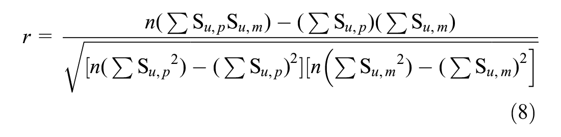
where n is the number of samples or observations, S_u,p is the predicted or estimated value, and S_u,m is the measured or observed value.

Results of ANN Modeling

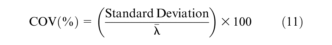
As shown above in Table 1, different types of ANN models with different input parameters were investigated. The input parameters primarily included q_t-avg. However, f_s-avg and some other easily achievable soil properties: σ_vo, LL, and PL, were also utilized in different combinations in conjunction with q_t-avg and f_s-avg. The objective was to perceive whether inclusion of these parameters as inputs would enhance the prediction capability of ANN models. For each ANN model type, different numbers of hidden layers and different numbers of nodes per hidden layer were tried to obtain the best-performing ANN model. A summary of the best-performing ANN models of each type (six model types in Table 1) in relation to predicting the measured undrained shear strength of soil (training, testing and validation) is listed in Table 2. As stated earlier, the performance was evaluated based on the coefficient of correlation, r, the coefficient of determination, R², the root mean square error, RMSE, mean bias factor, $λ,$ and the coefficient of variation, COV. The ANN models are designated in a manner to understand the structure of the model at a glance. For example, for the model designated as 2-6-4-1, the first and last number refers to the number of nodes in the input and output layers, respectively, meaning that the model has two input parameters with only one output parameter. The intermediate numbers denote the number of hidden layers and nodes, that is, the mentioned model has two hidden layers with six and four nodes, respectively.

Table 2.

Comparison of Artificial Neural Network (ANN) Models

ANN type	ANN model	Phase	r	R²	RMSE	Mean $λ$	COV
Type 1	2-6-4-1	Training	0.90	0.79	378.21	0.99	0.31
		Testing	0.92	0.81	456.28	0.96	0.40
		Validation	0.92	0.82	370.57	0.99	0.30
	2-5-3-1	Training	0.86	0.67	477.45	0.99	0.33
		Testing	0.86	0.69	392.52	0.90	0.38
		Validation	0.91	0.81	465.01	0.90	0.32
	2-5-1	Training	0.90	0.79	437.59	1.02	0.34
		Testing	0.78	0.49	446.09	0.99	0.44
		Validation	0.84	0.60	363.23	0.98	0.28
Type 2	3-8-1	Training	0.93	0.85	366.59	1.00	0.30
		Testing	0.87	0.69	379.88	0.98	0.29
		Validation	0.92	0.84	340.73	1.01	0.26
	3-4-4-1	Training	0.93	0.84	368.93	1.00	0.27
		Testing	0.84	0.64	464.07	0.87	0.43
		Validation	0.90	0.76	368.81	0.91	0.32
	3-6-6-1	Training	0.93	0.86	345.57	1.01	0.26
		Testing	0.84	0.66	457.90	0.88	0.40
		Validation	0.86	0.60	424.60	0.92	0.35
Type 3	2-2-2-1-1	Training	0.87	0.73	486.79	0.98	0.37
		Testing	0.85	0.69	412.74	0.97	0.35
		Validation	0.88	0.75	356.59	1.03	0.28
	2-6-2-1-1	Training	0.89	0.76	447.33	0.99	0.34
		Testing	0.80	0.58	486.44	1.05	0.34
		Validation	0.88	0.73	399.56	0.98	0.34
	2-6-4-1	Training	0.91	0.83	371.68	0.99	0.32
		Testing	0.86	0.73	570.79	1.00	0.41
		Validation	0.88	0.77	426.50	1.00	0.34
Type 4	1-6-1-1	Training	0.80	0.50	575.20	0.99	0.41
		Testing	0.77	0.52	629.06	1.12	0.41
		Validation	0.87	0.75	361.54	1.01	0.31
	1-5-5-3-1	Training	0.80	0.50	556.30	0.96	0.36
		Testing	0.84	0.66	467.89	0.90	0.42
		Validation	0.87	0.70	466.54	1.03	0.49
	1-6-5-3-1	Training	0.84	0.63	513.64	0.99	0.38
		Testing	0.85	0.68	442.83	0.93	0.39
		Validation	0.85	0.68	494.19	1.05	0.49
Type 5	4-3-2-1	Training	0.92	0.83	366.81	0.99	0.32
		Testing	0.88	0.75	526.71	1.13	0.28
		Validation	0.89	0.76	349.44	0.97	0.30
	4-4-3-2-1	Training	0.90	0.80	428.39	0.99	0.33
		Testing	0.87	0.63	406.62	0.80	0.33
		Validation	0.91	0.77	353.74	0.90	0.33
	4-5-1-1	Training	0.91	0.82	394.31	1.01	0.31
		Testing	0.87	0.68	424.38	0.81	0.32
		Validation	0.91	0.82	372.18	0.93	0.31
Type 6	5-4-3-1	Training	0.94	0.88	332.23	1.01	0.36
		Testing	0.84	0.63	409.50	0.96	0.53
		Validation	0.92	0.84	352.49	0.98	0.31
	5-4-3-2-1	Training	0.93	0.88	334.59	1.03	0.29
		Testing	0.81	0.67	468.51	0.96	0.33
		Validation	0.91	0.82	391.71	0.97	0.34
	5-4-3-3-1	Training	0.93	0.87	340.21	1.05	0.31
		Testing	0.87	0.68	406.53	0.94	0.38
		Validation	0.91	0.78	383.08	1.01	0.32

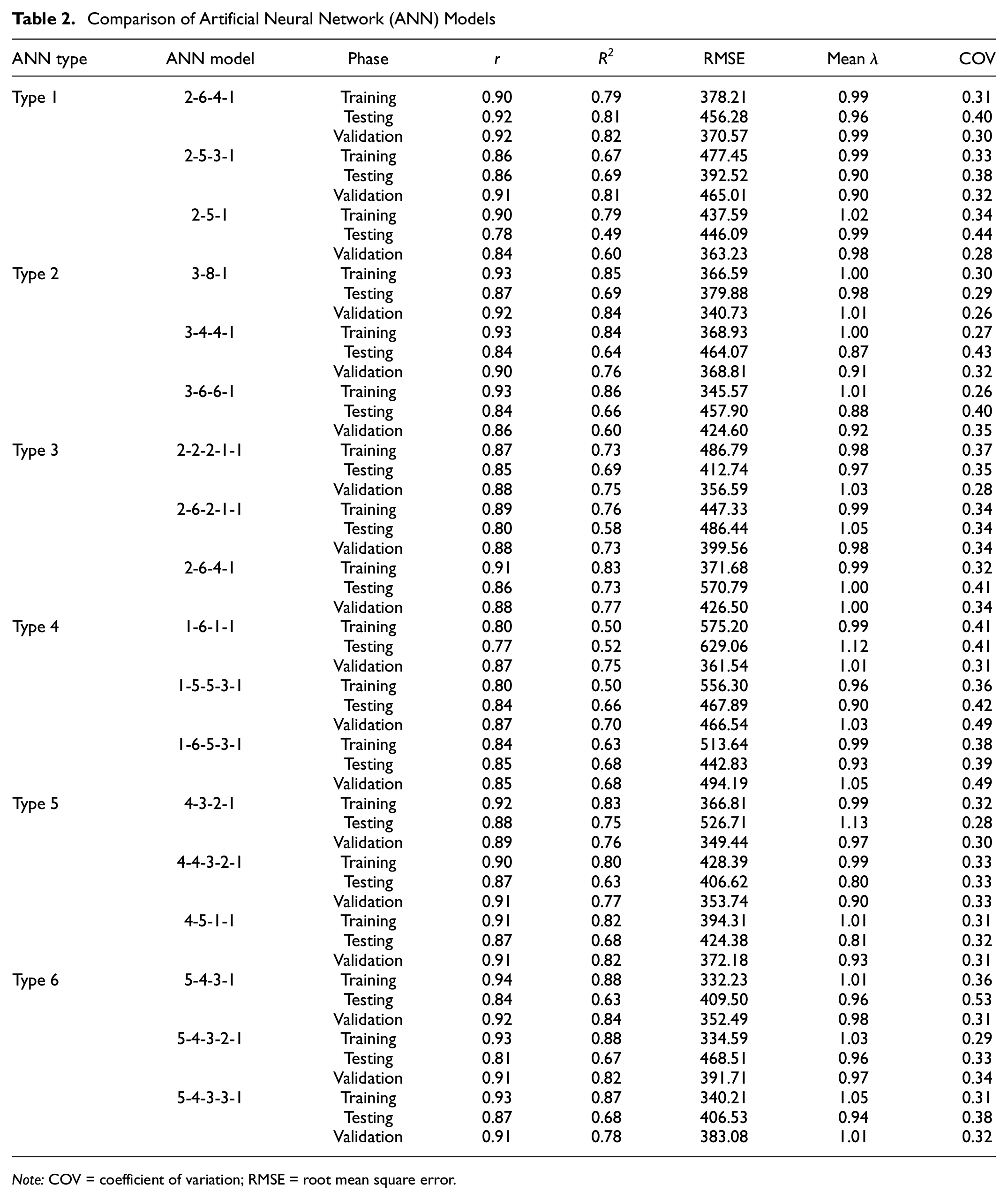
Note: COV = coefficient of variation; RMSE = root mean square error.

The ANN models listed in Table 2 represent the top three best-performing models of each type obtained through trial and error from hundreds of ANN models. It can be observed that Type 1 ANN model 2-6-4-1 (input parameters q_t-avg and f_s-avg only) has a good prediction capacity with quite satisfactory evaluation statistics (validation phase RMSE = 370.57 psf, r = 0.92, R² = 0.82, mean $λ$ = 0.99, COV = 0.30). However, an enhancement in the prediction capability was observed with the involvement of effective overburden pressure (σ_vo) as an input parameter in Type 2 ANN model 3-8-1, which is also in agreement with the literature ( 6 , 7 ). From Table 2, it is also obvious that Type 2 ANN model 3-8-1 is the best ANN model of this study based on its performance in the prediction of undrained shear strength of soil (S_u). Another ANN model, 5-4-3-1 of Type 6 (with q_t-avg, f_s-avg, σ_vo, LL, and PL as input parameters) shows promising S_u prediction results (validation phase RMSE = 352.49 psf, r = 0.92, R² = 0.84, mean $λ$ = 0.98, COV = 0.31), better than that of Type 1 ANN model 2-6-4-1. However, despite having a very good S_u prediction capability, Type 6 ANN model 5-4-3-1 was not considered to relieve the burden of added soil parameters as input. For the most part, it can be inferred from the results presented in Table 2 that the combination of q_t-avg and f_s-avg, along with σ_vo, yields the best ANN prediction models to evaluate the undrained shear strength of soil.

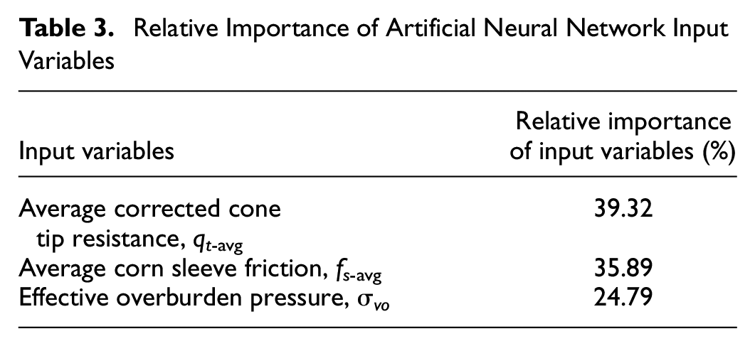
Sensitivity Analysis of ANN Input Parameters

Sensitivity analysis was performed on the input parameters for the best-performing ANN model 3-8-1 of Type 2 to evaluate the effect of these parameters (q_t-avg, f_s-avg, and σ_vo) on the output S_u. The results of sensitivity analysis are listed in Table 3, which shows that the average corrected cone tip resistance, q_t-avg, is relatively the most important input parameter. The results also show that the average sleeve friction, f_s-avg, also possesses significance importance in the prediction of S_u. However, the percentages of their relative importance indicates that all three input parameters play significant roles in better interpretation of the undrained shear strength of soil using the ANN models.

Table 3.

Relative Importance of Artificial Neural Network Input Variables

Input variables	Relative importance of input variables (%)
Average corrected cone tip resistance, q_t-avg	39.32
Average corn sleeve friction, f_s-avg	35.89
Effective overburden pressure, σ_vo	24.79

Comparison between ANN Model and Conventional Methods

The equation by Lunne and Kleven ( 6 ) modified with corrected tip resistance, q_t, has been used widely for decades to evaluate the undrained shear strength of soil from CPT parameters. The best-performing ANN model of this study, 3-8-1, was compared with this method with the same validation data set (see Table 4). Based on prior knowledge from the literature ( 36 , 37 ) and local experience ( 38 ), the N_kt value was considered to be 15.9 in the equation: $s_{u} = \frac{(q_{t} - σ_{vo})}{N_{kt}}$ . The comparison of results (Table 4, Figure 4) shows that the ANN model possesses relatively higher precision in the interpretation of shear strength of soil. Therefore, it can be deduced that the ANN models can substantially interpret the undrained shear strength of soil from CPT parameters.

Table 4.

Comparison of Artificial Neural Network (ANN) Model with Conventional Model

Method	r	R ²	RMSE	Mean $λ$	CoV
ANN (3-8-1)	0.92	0.84	340.73	1.01	0.26
Lunne and Kleven ( 6 )	0.89	0.74	378.09	0.97	0.32

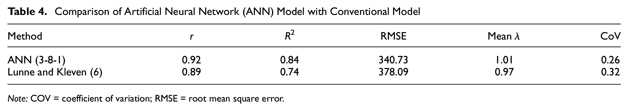
Note: COV = coefficient of variation; RMSE = root mean square error.

Figure 4.

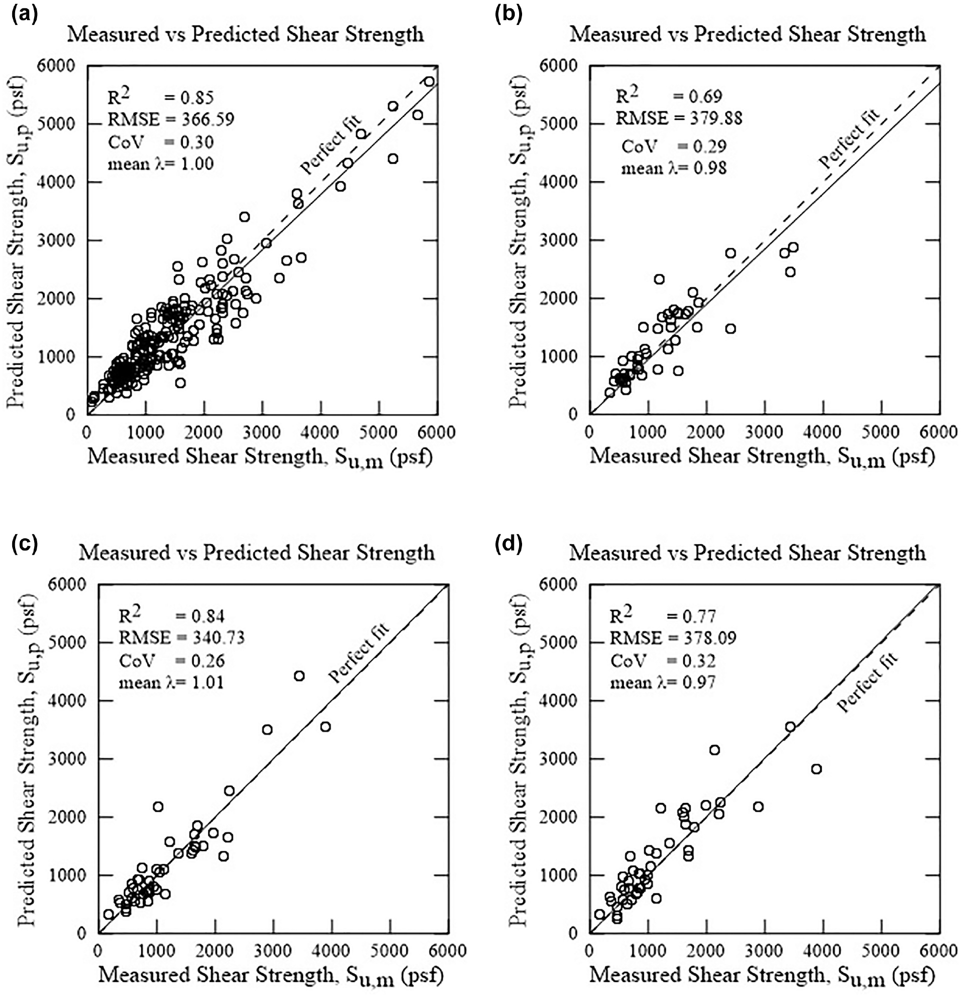
Predicted versus measured undrained shear strength of soil: (a) training; (b) testing; (c) validation phases of artificial neural network type 2 model 3-8-1; and (d) Lunne and Kleven ( 6 ). COV = coefficient of variation; RMSE = root mean square error.

Limitations

The ANN models were developed from a database collected from the Louisiana Department of Transportation and Development. The database of this study mostly represents clayey soils in Louisiana. Thus, the proposed ANN models should perform well for clayey soils of Louisiana, and other locations with similar geological conditions. However, it is recommended to follow the following guidelines at the time of using the ANN models:

It is to be noted that the ANN cannot extrapolate efficiently beyond the range of the training data. Therefore, the range of q_t should be ≤ 100,000 psf, the range of f_s should be ≤ 4,000 psf, and the range of σ_vo should be ≤ 9 18,000 psf, and the range of soil collection depth should be between 4 ft (1.2 m) to 110 ft (33.5 m).

The developed ANN models should be used only to predict the data for unknown sites without further training. If it is trained again on the same training data, the prediction capability might not remain the same.

Summary and Conclusions

ANN was used in this study to explore the potential of using artificial intelligence to accurately estimate the undrained shear strength of soil. A database consisting of CPT/PCPT data along with corresponding soil boring and laboratory test data from 70 test sites located in 14 different parishes in Louisiana was used in this study. Six types of ANN models with different combinations of input parameters (LL, PL, and σ_vo in conjunction with CPT parameters q_t-avg, f_s-avg) were explored to obtain the best model regarding the prediction of undrained shear strength of soil (S_u). For each ANN model type, different architectures (different numbers of hidden layers and different nodes per hidden layer) were tried to enhance the performance. Sensitivity analysis was performed to assess the relative importance of the CPT input parameters of the best performed model. In addition, the results of the ANN models were compared with the results of the widely used empirical equation published by Lunne and Kleve in 1981 ( 6 ) using the same validation data. Based on the findings of this study, the following conclusions can be drawn:

Almost all the developed ANN model types were able to estimate the measured undrained shear strength of soil with good to excellent accuracy. Type 1 ANN model 2-6-4-1 with only CPT parameters (q_t-avg, f_s-avg) as input, generated satisfactory prediction (validation phase: R² = 0.82 λ = 0.99, RMSE = 370.57 psf, COV = 0.30). However, with the inclusion of an easily obtainable soil property, effective overburden pressure (σ_vo) as input, Type 2 ANN model 3-8-1 (input parameters: q_t-avg, f_s-avg and σ_vo) turned out to be the best-performing ANN model of this study succeeding on all the evaluation criteria (validation phase: R² =0.84 λ = 1.01, RMSE = 340.73 psf, COV = 0.26). Besides, ANN model 5-4-3-1 of Type 6 (q_t-avg, f_s-avg, σ_vo, LL and PL as input parameters) also showed promising prediction results (validation phase RMSE = 0.352.49 psf, r = 0.92, R² = 0.84, mean $λ$ = 0.98 and COV = 0.31) which is better than that of the Type 1 ANN model. From the results, therefore, it is obvious that the ANN algorithm can be successfully implemented to estimate the undrained shear strength of soil from CPT data.

The results of ANN analyses showed that using the combination of a few soil properties that is, LL, PL and σ_vo as inputs, along with average corrected tip resistance, q_t-avg, and average sleeve friction, f_s-avg, facilitated the ANN model to better grasp the relation between input parameters and the output, measured undrained shear strength of soil.

Sensitivity analysis of the ANN Type 2 model 3-8-1 showed that the average corrected cone tip resistance, q_t-avg, has relatively the highest importance among the three input parameters (q_t-avg, f_s-avg and σ_vo). However, the percentages of relative importance of all three input parameter indicates that all play significant roles in better interpretation of the undrained shear strength of soil using the ANN models.

Comparison of between the best-performing ANN model (3-8-1) and the widely implemented empirical equation by Lunne and Kleven ( 6 ), using the same validation data, clearly showed that the ANN model outweighed the performance of conventional empirical methods in the estimation of the undrained shear strength of soil.

Finally, the estimation of undrained shear strength of soil is cumbersome in many cases because of difficulty in obtaining undisturbed soil samples and performing the relatively strenuous triaxial test. Although the problem can be solved using mathematical models, these involve correlation equations that require different assumptions and judgments. In contrast, the ANN uses only data from previous experience and training without incorporating such assumptions or hypotheses. Furthermore, the ANN models can be continuously updated over time to achieve more accurate estimation results, if new input data is available.

Footnotes

Acknowledgements

The authors are grateful to Louisiana Department of Transportation and Development engineers for providing valuable help and support in this study.

Author Contributions

The authors confirm contribution to the paper as follows: study conception and design: M. Abu-Farsakh, M.A.H. Mojumder; data collection: M.A.H. Mojumder; analysis and interpretation of results: M.A.H. Mojumder, M. Abu-Farsakh; draft manuscript preparation: M.A.H. Mojumder, M. Abu-Farsakh. Both authors reviewed the results and approved the final version of the manuscript.

Declaration of Conflicting Interests

The author(s) declared no potential conflicts of interest with respect to the research, authorship, and/or publication of this article.

Funding

The author(s) disclosed receipt of the following financial support for the research, authorship, and/or publication of this article: This research project is funded by the Louisiana Transportation Research Center (LTRC Project No. 17-2GT) and Louisiana Department of Transportation and Development (State Project No. DOTLT1000165).

References

Huang

Sheng

Sloan

S. W.

H. S.

Finite Element Analysis of Cone Penetration in Cohesionless Soil. Computers and Geotechnics, Vol. 31, No. 7, 2004, pp. 517–528.

Abu-Farsakh

Tumay

Voyiadjis

Numerical Parametric Study of Piezocone Penetration Test in Clays. International Journal of Geomechanics, Vol. 3, No. 2, 2003, pp. 170–181.

H. S.

Whittle

A. J.

Combining Strain Path Analysis and Cavity Expansion Theory to Estimate Cone Resistance in Clay. Unpublished Notes, 1999.

Salgado

Boulanger

R. W.

Mitchell

J.K.

, Lateral Stress Effects on CPT Liquefaction Resistance Correlations. Journal of Geotechnical and Geo-Environmental Engineering, Vol. 123, No. 8, 1997, pp. 726–735.

Teh

C. I.

Houlsby

G. T.

An Analytical Study of the Cone Penetration Test in Clay. Geotechnique, Vol. 41, No. 1, 1997, pp. 17–34.

Lunne

Kleven

Role of CPT in North Sea Foundation Engineering. Proc., Cone Penetration Testing and Experience, ASCE, St. Louis, MO, 1981, pp. 76–107.

Senneset

Janbu

Svano

Strength and Defomation Parameters from Cone Penetrometer Tests. Proc., 2nd European Symposium on Penetration Testing ESOPT II, Amsterdam, Vol. 2, 1982, pp. 863–870.

Shahin

M. A.

Maier

H. R.

Jaksa

M. B.

Predicting Settlements of Shallow Foundations using Neural Networks. Journal of Geotechnical and Geoenvironmental Engineering, Vol. 128, No. 9, 2002.

Neaupane

K. M.

Achet

S. H.

Use of Backpropagation Neural Network for Landslide Monitoring: A Case Study in the Higher Himalaya. Engineering Geology, Vol. 74, No. 3–4, 2004, pp. 213–226.

10.

Das

S. K.

Basudhar

P. K.

Undrained Lateral Load Capacity of Piles in Clay using Artificial Neural Network. Computers and Geotechnics, Vol. 33, No. 8, 2006, pp. 454–459.

11.

Pooya Nejad

Jaksa

M. B.

Reza Kakhi

McCabe

B. A.

Prediction of Pile Settlement using Artificial Neural Networks Based on Standard Penetration Test Data. Computers and Geotechnics, Vol. 36, No. 7, 2009, pp. 1125–1133.

12.

Shahin

M. A.

Jaksa

M. B.

Maier

H. R.

Recent Advances and Future Challenges for Artificial Neural Systems in Geotechnical Engineering Applications. Advances in Artificial Neural Systems, Vol. 2009, 2009, pp. 1–9.

13.

Ikizler

S. B.

Aytekin

Vekli

Kocabaş

Prediction of Swelling Pressures of Expansive Soils using Artificial Neural Networks. Advances in Engineering Software, Vol. 41, No. 4, 2010, pp. 647–655.

14.

Pooya Nejad

Jaksa

M. B.

Load-Settlement Behavior Modeling of Single Piles using Artificial Neural Networks and CPT Data. Computers and Geotechnics, Vol. 89, 2017, pp. 9–21.

15.

Shahin

M. A.

Jaksa

M. B.

Intelligent Computing for Predicting Axial Capacity of Drilled Shafts. Proc., Contemporary Topics in In Situ Testing, Analysis, and Reliability of Foundations, Orlando, FL, 2009, pp. 26–33.

16.

Basheer

I. A.

Hajmeer

Artificial Neural Networks: Fundamentals, Computing, Design, and Application. Journal of Microbiological Methods, Vol. 43, 2000, pp. 3–31.

17.

Rumelhart

D. E.

McClleland

J. L.

Learning Internal Representation by Error Propagation. MIT Press, Cambridge, MA, 1986.

18.

Basheer

I. A.

Neuromechanistic-Based Modeling and Simulation of Constitutive Behavior of Fine-Grained Soils. PhD dissertation. Kansas State University, Manhattan, KS, 1998.

19.

Hammerstrom

Working with Neural Networks. IEEE Spectrum, Vol. 30, No. 7, 1993, pp. 46–53.

20.

Stone

Cross-Validatory Choice and Assessment of Statistical Predictions. Journal of the Royal Statistical Society. Series B (Methodological), Vol. 36, No. 2, 1974, pp. 111–147.

21.

Shahin

M. A.

Maier

H. R.

Jaksa

M. B.

Data Division for Developing Neural Networks Applied to Geotechnical Engineering. Journal of Computing in Civil Engineering, Vol. 18, No. 2, 2004.

22.

Looney

C. G.

Advances in Feedforward Neural Networks Demystifying Knowledge Acquiring Black Boxes. IEEE Transactions, on Knowledge and Data Engineering, Vol. 8, No. 2, 1996, pp. 211–226.

23.

Flood

Kartam

Neural Networks in Civil Engineering I: Principles and Understanding. Journal of Computing in Civil Engineering, Vol. 8. No. 2, 1994.

24.

Cybenko

Approximation by Superpositions of a Sigmoidal Function. Mathematics of Control, Signals, and Systems, Vol. 2, 1989, pp. 303–314.

25.

Hornik

Stinchcombe

White

Multilayer Feed-Forward Networks Are Universal Approximators. Neural Networks, Vol. 2, 1989, pp. 359–366.

26.

Ripley

B. D.

Pattern Recognition via Neural Networks. Cambridge University Press, Cambridge, 1996.

27.

Lapedes

Farber

How Neural Nets Work. Neural Information Processing Systems, American Institute of Physics, D.Z. Anderson, New York, 1988, pp. 442–456.

28.

Chester

Why Two Hidden Layers Are Better Than One. International Joint Conference on Neural Networks, Washington D.C., Vol. 1, 1990, pp. 265–268.

29.

Masters

Practical Neural Network Recipes in C++. Academic Press, San Diego, CA, 1993.

30.

Shahin

M. A.

Jaksa

M. B.

Maier

H. R.

State of the Art of Artificial Neural Networks in Gerotechnical Engineering. Electronic Journal of Geothechnical Engineering, Vol. 13, 2008, pp. 1–26.

31.

Salchenberger

L. M.

Char

E. M.

Lash

N. A.

Neural Networks a New Tool for Predictiong Thrift Failures. Decision Science, Vol. 23, 1992, pp. 899–916.

32.

Berke

Hajela

Application of Neural Networks in Structural Optimization. NATO/AGARD Advanced Study Institute, Il Cicocco, Italy, Vol. 23, No. I–II, 1991, pp. 731–745.

33.

Hecht-Nielson

Kolmogrov’s Mapping Neural Network Existence Theorem. Proc., 1st IEEE International Joint Conference on Neural Networks, San Diego, CA, 1987.

34.

Nawari

N. O.

Liang

Nusairat

Artificial Intelligence Techniques for the Design and Analysis of Deep Foundations. Electronic Journal of Geotechnical Engineering, Vol. 4, 1999, pp. 1–21.

35.

Smith

G. N.

Probability and Statistics in Civil Engineering: An Introduction. Collins, London, 1986.

36.

Robertson

P. K.

Interpretation of Cone Penetration Tests — A Unified Approach. Canadian Geotechnical Journal, Vol. 46, No. 11, 2009, pp. 1337–1355.

37.

Mayne

P. W.

Cone Penetration Testing: NCHRP Synthesis 368. Transportation Research Board, Washington, D.C., 2007.

38.

Hossain

M. I.

Abu-Farsakh

M. Y.

Evaluation of Undrained Shear Strength from Cone Penetration Test. Presented at 98th Annual Meeting of the Transportation Research Board, Washington, D.C., 2019.