Person-Based Micro-Simulation Demand Model for National Long-Distance Travel in the U.S.A.

Abstract

As the nation and various states engage in funding transportation infrastructure improvements to meet future long-distance passenger travel demand, it is imperative to develop effective and practical modeling methods for analysis of long-distance passenger travel. Evaluating national-level infrastructure improvements requires a reliable analysis tool to model the demand for long-distance travel. The national travel demand model presented in this paper implements a person-level tour-based micro-simulation approach for modeling individuals’ long-distance or national activities in the U.S.A. This paper reviews the model framework, explains the model calibration, and presents applications of the model for policy evaluation and demand prediction. The model was estimated using the latest long-distance travel survey in the U.S.A., which is the 1995 American Travel Survey. As the estimation data is old, and no new long-distance travel survey with appropriate sample size is available to re-estimate the model, model calibration is the solution used to update the model and make it capable of capturing up-to-date travel patterns. Calibrating such a large-scale model can be challenging, because each calibration iteration is very costly. This paper describes the calibration effort conducted on the national long-distance micro-simulation model to showcase how a large-scale travel demand model can be calibrated efficiently. A fuel price scenario is analyzed to show how the national travel demand will change under a national fuel price increase scenario in the future year 2040. Another scenario analysis corresponding to construction of high-speed rail (HSR) is conducted to observe the effects of adding a HSR system to the northeast corridor on travel demand from a national perspective.

The increasing interest in national transportation policies, from strategic infrastructure investment to infrastructure operation and management with regard to efficiency, sustainability, and safety, has incited researchers and decision makers to call for advanced and policy-sensitive tools ( 1 ). Decisions such as highway infrastructure investment, high-speed rail construction, and airport development depend on national travel patterns. Some major infrastructure investments or operational and management improvements should be evaluated through a capable national travel analysis tool instead of state-level, region-level, or corridor-level models.

National long-distance passenger travel demand analysis has been an understudied area in transportation planning. The lack of multi-modal, long-distance, origin–destination data or appropriate national long-distance surveys has seriously limited modelers’ ability to develop a national long-distance model. As the nation and various states engage in funding transportation infrastructure improvements to meet future long-distance passenger travel demand (interstate highway tolling/expansion, high-speed rail, and a next-generation passenger air transportation system that relies more on smaller airports and aircraft), developing national long-distance models should be a priority. There are significant differences between long-distance trips and daily/weekly trips modeled in the metropolitan/state-level tour/activity-based models ( 2 ). For instance, long-distance trips usually take days or weeks and may involve car, airplane, train, bus, or a combination of modes. Households tend to choose the time of travel for long-distance vacation trips based on time and budget before selecting destination and mode. Trip purpose categories are also different for long-distance trips. Cost of travel for long-distance trips should include lodging, food, and so on. The same applies to the total travel time for long-distance travel, which should cover not only in-vehicle travel time but also the access/egress time, transfer time, and lodging time. The lower frequency of long-distance travel may also imply a different decision-making process. These differences highlight the need for an independent national long-distance model that can address these differences.

After the Intermodal Surface Transportation Efficiency Act (ISTEA) (3, 4) was enacted in 1991, many state departments of transportation (DOTs) began developing statewide travel demand models as critical analysis tools for addressing legislative requirements in statewide planning. However, the statewide models are usually weak in external/internal (EI) or internal/external (IE) trips that require data from federal and neighboring states ( 5 ). A significant part of the IE and EI trips are long-distance travels. There are also external/external (EE) trips that may use a state’s highway system. These trips are also related to long-distance travel. According to Giaimo and Schiffer’s review ( 6 ) of developments in statewide travel demand modeling, most statewide travel demand models in the U.S.A. do not consider long-distance travel. A national long-distance travel demand model can provide external trips for statewide models in the base year and future years. During the years since that review, the situation has been changed. Today, several states have active modeling efforts considering long-distance travel to meet statewide policy and legislative development needs. Examples can be found in California, Ohio, Maryland, and Kentucky. The California Statewide Travel Demand Model is a tour-based travel demand model that can forecast all types of travel made by California residents, whether short or long distance ( 7 ). Ohio’s statewide travel demand model uses a state-of-the-art tour-based modeling approach. It models both short-distance and long-distance (longer than 50 mi) travels. The long-distance travel models are developed based on the Ohio DOT’s sponsored long-distance travel survey data and can estimate the frequency and characteristics of long-distance travels ( 8 ). The Maryland Statewide Transportation Model version 1.0 is a four-step travel demand model which includes a regional component that models long-distance travels made by residents and visitors ( 9 ). Maryland recently upgraded its travel demand model to version 2.0, which utilizes the national long-distance model presented in this paper ( 10 ). The Kentucky Statewide Travel Demand Model models long-distance trips (over 100 mi) in Kentucky and parts of the neighboring states. The model adopts a modified four-step travel demand model, removing the mode choice module ( 11 ). Even though many recent statewide travel models consider long-distance travels, the long-distance travels are not their focus. They are usually weak in modeling EE trips, or very long IE/EI trips. Generally, a statewide model focusing on one state and its adjacent regions is not a sufficient tool for evaluating national and federal policies. Because of the need for national policy evaluation tools, the National Cooperative Highway Research Program (NCHRP) supported a scoping study for developing a national travel forecasting model, led by Cambridge Systematics ( 5 ). NCHRP later supported an effort to develop national origin–destination (OD) tables, led by CDM Smith ( 12 ). These efforts led to the Federal Highway Administration’s (FHWA) Exploratory Advanced Research (EAR) program supporting a project to develop a national travel demand modeling framework, led by Resource Systems Group (RSG) (13, 14). The EAR program project led to the only available national tour-based travel demand modeling framework, besides the one presented in this paper. One of the main reasons for insufficient efforts in modeling long-distance national travels in the U.S.A. is the lack of recent data resources. The American Travel Survey (ATS) was a survey dedicated to long-distance travel, but it was conducted only once, in 1995. This 1995 ATS is the only source of long-distance travel survey data with sufficient sample size to estimate all components required in a long-distance travel demand model. Later National Household Travel Surveys included long-distance trips, but the long-distance sample size was considerably smaller than in the ATS, not enough to estimate a comprehensive long-distance travel demand model. Furthermore, the available large-scale national surveys are cross-sectional. Recent studies using a longitudinal survey of overnight travel ( 2 ) suggest that many aspects of long-distance travel may not be captured without longitudinal surveys ( 15 – 17 ).

The national long-distance model presented in this paper is a person-level tour-based micro-simulation travel demand model for national travel analysis. All major behavioral dimensions of long-distance travel are considered in this model. Compared with the traditional four-step approach, tour-based techniques offer several advantages: (i) it is easier to consider tours, multi-day and multi-stop trips, and intermodal access/egress transfers that are important for long-distance travel modeling; (ii) households and persons are the basic units of analysis, which enables modeling of detailed behavioral representations and interactions; and (iii) it provides a rich framework for analysis of travel as a multi-day, monthly, quarterly, or yearly pattern of behavior, derived from activity participation. The long-distance model simulates activities and trips at the Metropolitan Statistical Area (MSA)/Non-MSA-level, which is the highest geographic resolution in the long-distance travel survey data. The model system is developed considering the specific attributes of long-distance travel, such as low frequency, long activity duration, different sets of mode alternatives, and so on. The model system not only considers an individual’s long-distance travel at the tour level, but also at the stop level. The model is implemented in our developed micro-simulation platform, which simulates each individual’s yearly long-distance activities and travel in the U.S.A. over the course of one year based on a synthetic population dataset.

The contribution of this paper is in presenting an integrated activity-based travel demand model system for individuals’ quarterly/yearly long-distance travels considering the specific attributes of long-distance travels. The model offers a strong policy evaluation tool that can provide important insights into the nation’s long-distance travels and help guide federal and state agencies with making decisions on corridor-level, region-level, and nation-level infrastructure investment, design, and management. The paper presents how important national-level policies such as fuel price increase or multi-state projects such as high-speed rail can be evaluated. The modeling tool introduced can help decision makers and politicians evaluate and design such policies systematically and quantify their effects on different population groups or different regions, as shown in the two application examples of this paper. FHWA has planned the next iteration of the National Household Travel Survey with a passively collected data component to produce national OD tables. Such continuous national-level data can help monitor national travel trends and lead to more national-level studies. The combination of national passively collected data products to monitor the status quo of national travel demand and a national person-level micro-simulation tool to evaluate project and policy alternatives and to project future travel demand can serve as a comprehensive toolbox to inform decision-making at the national level.

In the next section, a review of the model framework is presented. The following section describes how such a large-scale model can be calibrated efficiently. Two future year scenario testing results are then presented to showcase the model’s applications. One application is focused on a fuel price increase scenario; the other is focused on adding a high-speed rail mode to the northeast corridor. The last section of the paper presents a summary and conclusion.

Model Overview

The tour-based national travel demand model developed by the authors can forecast the long-distance passenger tours made by auto, air, and train in the U.S.A. over a one-year period using a micro-simulation framework. A long-distance trip in the model system is defined as a trip longer than or equal to 50 mi, one way. This definition is based on the distance-based definition of trips in the ATS. This can be seen as a limitation of this paper based on the recent research arguing against the use of distance-based definitions of long-distance trips (15, 18). Definition of long-distance trips is still a critical challenge in the field. For each long-distance tour in our modeling framework, there is only one tour destination or primary destination, and during each leg of the tour, there could be multiple intermediate stops. The model system consists of three tiers. The first is the yearly long-distance activity pattern level, which predicts the number of different types of activities a person will choose during one year. The second is the tour-level model system, which contains choices of tour destination, time of year, tour duration, and tour mode; and the third is the stop-level model system, including the number, the purpose, and the location of each intermediate stop made during the inbound and outbound legs of the tour.

The yearly long-distance tour schedule can be presented as a set of different long-distance tours per year. The activity pattern model is responsible for generating the long-distance tour rates by purpose (business, personal business, pleasure) for each person using the multiple classification analysis method. After deriving how many long-distance tours each person makes, the next step is to predict the tour characteristics, namely mode, destination, time of year, and duration. Each of these attributes is predicted using a choice model. Figure 1 shows the model hierarchy for different tour purposes. The solid arrows indicates that the output of the upper level can be used as an explanatory variable at the lower level, while the dashed arrows mean that the expected utility of the lower-level models can affect the choices at the upper level. The hierarchy structure is different between business and pleasure tours. A long-distance pleasure tour requires people to consider their time availability before other decisions. When they have a period of time for pleasure, they will decide when to spend it, where to go, and how to go, sequentially. In contrast, people engaging in long-distance business and personal business activities usually give priority to the decision of the tour location and time, including the time of year and duration, followed by the tour mode choice. All of these model components use either discrete choice models or duration model.

Figure 1.

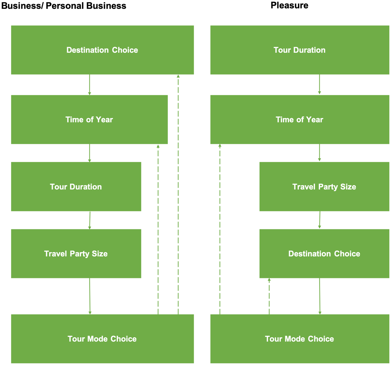
Tour-level procedure and model components.

After individuals have made decisions about their travel to the main destination, they will make plans for their trips on the way to and from the destination. The stop-level structure predicts the information of the intermediate stops people would make during the inbound/outbound legs of the long-distance tour. The stop frequency model at the higher level determines the number of intermediate stops people will make on the way to/from the tour destination. Once the number of stops on each tour leg is obtained, the purpose for each stop must be determined; the stop purpose categories follow the same tour-level purposes, which are business, personal business and pleasure. The location for each stop is predicted with the similar method employed in the primary destination choice at the tour level.

The model estimation is based on the 1995 ATS data ( 19 ). The ATS data provides detailed long-distance travel information, including the origin and destination of the trip, stops along the way to and from the destination, side trips originating at the destination, the means of transportation, the reason of the trip, the lodging type, the number of nights spent away from home, travel party size, and so on. The 1995 ATS is the only source of long-distance travel survey data with sufficient sample size to estimate all components required in a long-distance travel demand model. A later National Household Travel Survey (NHTS 2001) included long-distance trips, but the long-distance sample size was considerably smaller than that of ATS, not enough to estimate a comprehensive long-distance travel demand model. The 1995 ATS is dedicated to long-distance travel with appropriate sample size for building a long-distance travel demand model. This dataset was used in this study to estimate sets of econometric models on long-distance travels. The details of the model components and estimation results can be found in previous works by the authors (20, 21).

The person-based micro-simulation national travel demand model predicts the travel behavior of individuals aged 18 years or older. Each individual makes decisions based on his or her socio-demographic characteristics; therefore, it is necessary to synthesize the population in a way that best represents the real decision makers. Population synthesis is a procedure that expands the sample drawn from a population to the full population, such that the synthesized population can be representative of the actual population at various aggregate levels. The main idea of the population synthesis is to combine the census sample data (both household and person) with available up-to-date aggregate distribution or margins data. There are many population synthesizers using different methods for generating population. Here, PopGen is used, which is a standalone open-source software package developed by Arizona State University to generate the population of the entire U.S.A. by using distributions of household and person variables of interest, as well as a sample of household and person data ( 22 ). The sample data is based on 2006–2010 American Community Survey (ACS) five-year Public Use Microdata Sample (PUMS) data and the marginal data is obtained from the 2008–2012 ACS five-year summary files ( 23 ).

The model system is implemented in a micro-simulation platform developed by the authors using Java, which simulates individuals’ yearly long-distance activities and travel in the U.S.A. with the input of synthetic population data obtained from PopGen ( 22 ), the associated transportation OD skim data, and economic/demographic data. Even though the micro-simulation model can use the up-to-date population, land use, and skim inputs, it is still challenging for us to trust the results of a model estimated with a dataset collected in 1995. Travelers’ preferences may have changed because of new technologies, new lifestyles, and travel trends. This highlights the need for a calibration effort. The mode and time-of-year components of the model were calibrated using airline OD data (DB1B) and calibrating the destination choice component of the model using the most recent National Household Travel Survey (NHTS 2017). The calibration effort is described in the next section.

Model Calibration

Model calibration involves the optimization of model coefficients to match statistics obtained from an independent ground-truth dataset. The direction of change in the parameter space in each step can be obtained from the gradient. In many applications, such as the case of the long-distance model, a mathematical representation of the problem to calculate the gradient is not available. Consequently, information on the direct measurement of the gradient vector is not available. In such cases, the gradient can be approximated from measurements of the objective function ( 24 ).

In the calibration of the micro-simulation national long-distance model, because of the many sub-models embedded in the model, there is no simple closed-form mathematical relationship between model coefficients and model results. As a result, gradient needs to be approximated. The gradient approximation requires measuring the objective function at two adjacent points. Here, the objective function is the measure of the difference between simulation results and independent ground-truth data (statistics obtained from up-to-date travel surveys). The micro-simulation model simulates about 350 million individuals, which requires many computations, and takes a lot of time. Therefore, measuring the objective function for each step of the optimization is very costly. This highlights the need for a very efficient optimization algorithm.

Simultaneous perturbation stochastic approximation (SPSA) is an efficient method used in many complex multivariate optimization applications (25, 26). The algorithm is very efficient, in that its gradient approximation only requires two measurements of the objective function. SPSA has been applied in transportation to calibrate traffic simulation models (27, 28), calibrate traffic assignment models (29, 30), OD calibration (31, 32), and demand model estimation using machine-learning ( 33 ). Here, we first calibrated the model using the National Household Travel Survey (NHTS) from 2017, and then calibrated the model using the 2017 airline ticket DB1B data from the Bureau of Transportation Statistics.

NHTS is the source of information about the travel behavior of U.S. residents. The dataset includes information about households, individual travelers, individual trips, and vehicles. The latest NHTS, conducted in 2017, is the eighth in the NHTS series. The survey is collected from a representative sample of U.S. residents of 50 states plus the District of Columbia through address-based sampling. This dataset can be used to find useful information about travel behavior. The trip table of NHTS was first filtered to include only long-distance trips (longer than 50 mi). The sample was expanded to the entire population using trip weights. The number of long-distance trips attracted to each state was calculated afterward. The share of trips attracted to each state was calculated by dividing these numbers by the total number of long-distance trips. Therefore, the survey was summarized into 51 values representing the share of each state in trip attraction. Model simulation results were also summarized to produce the same values. The sum of the squared differences between model simulation result summaries and values obtained from NHTS for the 51 states was used as the objective function of the calibration against NHTS.

The DB1B data, collected by the office of Airline Information of the Bureau of Transportation Statistics, is a 10% sample of airline tickets. This dataset is collected from reporting carriers, and includes information about the origin and the destination of passengers. The dataset is usually used to understand air traffic patterns and passenger flows. The survey started in 1993, and contains quarterly information from 1993 to 2019. The coupon tables in the DB1B dataset include information about each flight. This dataset can be used to find the number of air trips originating from or attracted to each state. The market data for four quarters of 2017 was obtained and summarized to the following three values for each quarter: number of flights departing from Maryland, number of flights landing in Maryland, and total number of nationwide flight trips. Model simulation results were also summarized to produce the same values. The sum of the squared differences between model simulation result summaries and values obtained from DB1B for these 12 variables was used as the objective function of the calibration against DB1B.

For each calibration effort, the initial step involves specifying the calibration parameters. These are the parameters to be changed in the optimization process. For the calibration with the DB1B, the calibration was conducted to match the number of air trips in each quarter. The mode choice model can shift trips between modes and the time-of-year model can shift trips between quarters; therefore, changing the coefficients in the mode choice model and the time-of-year choice model can affect the number of air trips in each quarter. Among all model parameters in the mode choice and time-of-year choice models, alternative specific constants were selected as the calibration parameters, because changing these parameters has direct effects on the market shares for each quarter and each mode.

For the calibration with NHTS, the calibration was conducted to match the percentage of the total trips attracted to each state (trip attraction calibration). The destination choice model can shift the destination of trips between states; therefore, changing the coefficients in the destination choice model can affect the shares of total trips attracted to each state. The trip distribution model in our long-distance model does not have alternative specific constants. The main variables in the trip distribution model are: distance to destination, household density of the destination, and employment density of the destination. Consequently, we selected the distance coefficient, the household density coefficient, and the employment density coefficient in the destination choice models as the calibration parameters. These models are separated by trip purpose (pleasure, business, personal business); therefore nine parameters were selected for this calibration.

Another important aspect of the calibration is hyper-parameter selection for the SPSA algorithm. SPSA includes five hyper-parameters: a, c, α, γ, and A. More information about these parameters can be found in Spall’s book ( 25 ). These parameters were selected based on the suggestions in the optimization literature using the variance of the objective function, and the average of gradients.

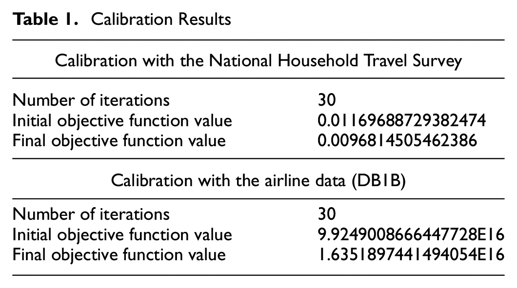
Table 1 shows the number of iterations, the initial objective function value, and the final objective value for each calibration effort. We can see significant improvements of the objective function (about 20% in NHTS calibration, about 80% in DB1B calibration). These improvements are obtained with as few as 30 iterations. A small number of iterations may raise some questions about the convergence of the optimization algorithm but the trend of the objective function in the two calibration efforts shows that the algorithm has converged (Figures 2 and 3). Readers can refer to Ghader et al. ( 34 ) for more information about the calibration of the model.

Table 1.

Calibration Results

Calibration with the National Household Travel Survey
Number of iterations	30
Initial objective function value	0.01169688729382474
Final objective function value	0.0096814505462386
Calibration with the airline data (DB1B)
Number of iterations	30
Initial objective function value	9.9249008666447728E16
Final objective function value	1.6351897441494054E16

Figure 2.

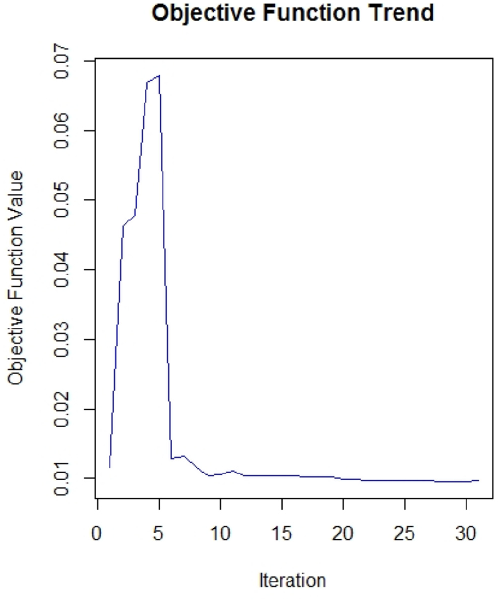
Objective function trend for calibration with National Household Travel Survey.

Figure 3.

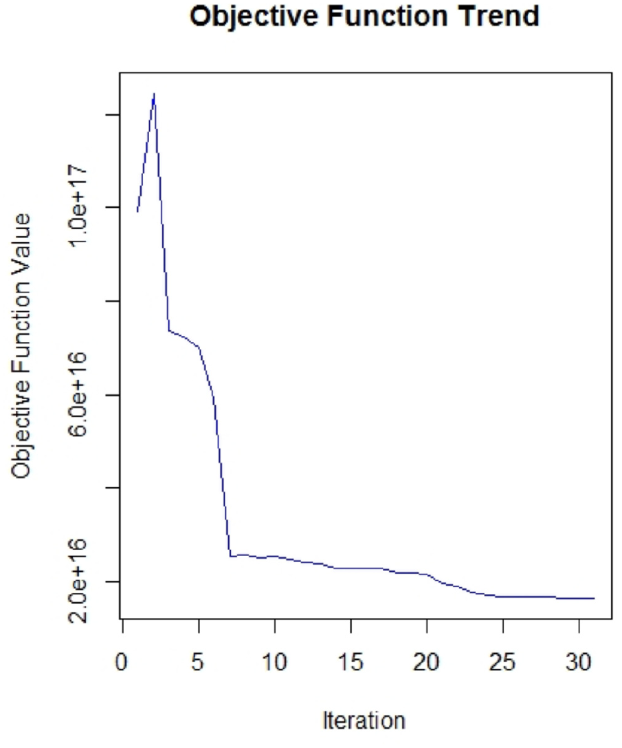
Objective function trend for the calibration with airline data (DB1B).

We acknowledge that a more comprehensive calibration using an up-to-date detailed dataset of long-distance trips can improve the model. The research team is currently further calibrating this model using national OD tables derived from passively collected data as a part of an FHWA EAR program project.

Base Year Model

The model’s base year is 2012. The zone structure of the model is at MSA level. The remaining part of each state not belonging to any MSA is considered as one non-MSA zone. Quarterly trip tables produced by the long-distance model contain the number of trips during the entire quarter for each combination of purpose and mode between each two zones.

In the model run for the 2012 base year, the car mode had the highest mode share, with about 90%, while air had 10% of the share, and rail had less than 1%. The shares of different trip purposes were 52% for pleasure, 32% for business, and 16% for personal business. The results also show that 47% of business trips used air mode while this number shrinks to 10% in the case of pleasure trips, meaning that car was a more popular choice when the trip purpose is pleasure. Based on the OD results, we can obtain long-distance trips to/from each MSA/non-MSA zone (Figure 4) for the nation. For year 2012, a total of 2.8 billion long-distance trips were made by the whole population, meaning that each person made about nine long-distance trips in one year.

Figure 4.

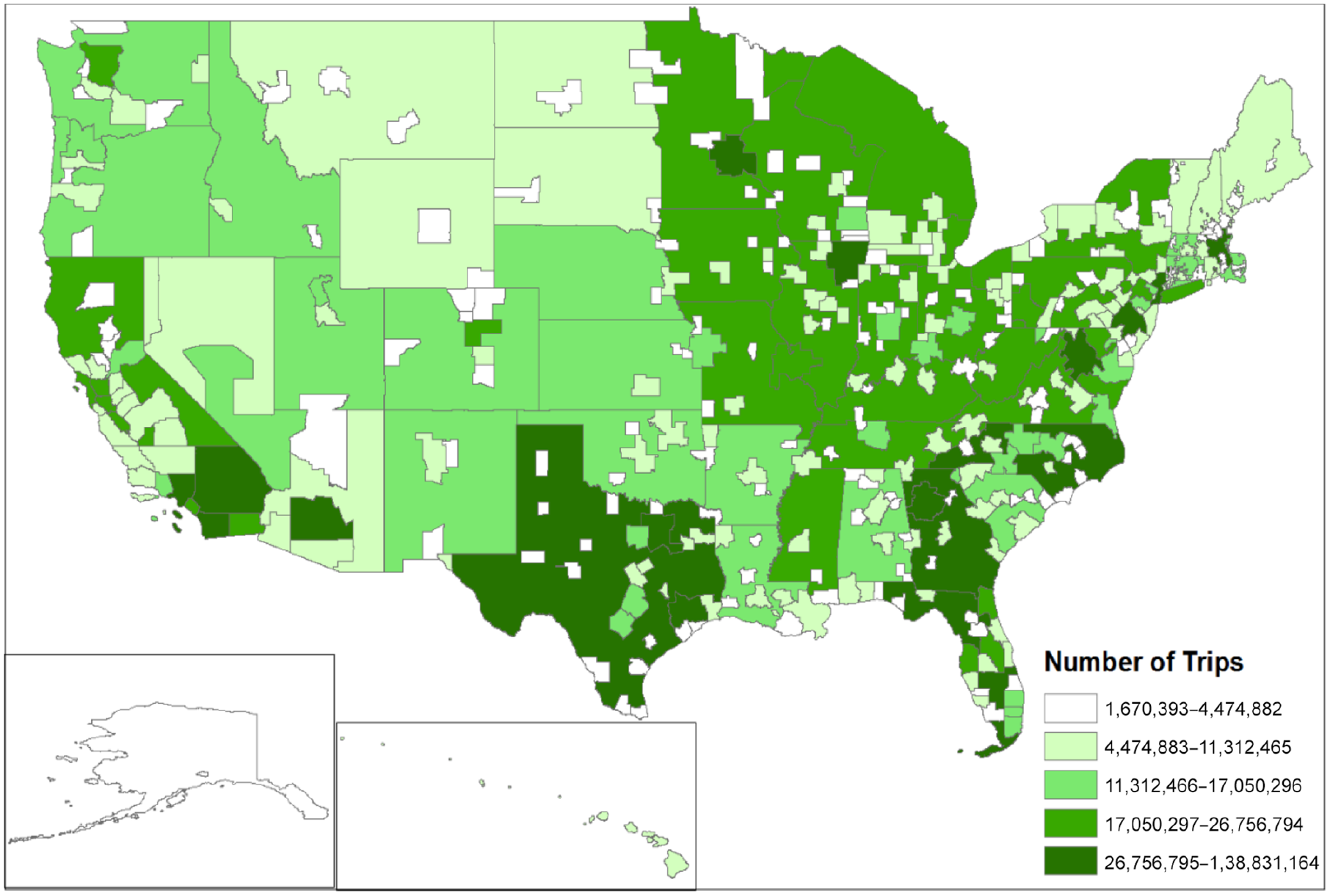
Trip generation at Metropolitan Statistical Area (MSA) and non-MSA-level.

Figure 5 shows the distribution of long-distance trips originating from Maryland to other states and coming from other states to Maryland for both car trips and air trips. Only the 10 states with the highest trip rates are shown. As expected, the states closer to Maryland, such as Pennsylvania, Virginia, and New York, had the most car trips and the distributions are the same for both trip attraction and generation. The model results show that for air trips, states with the highest population, such as Texas, California, and Florida, had the greatest share of trips.

Figure 5.

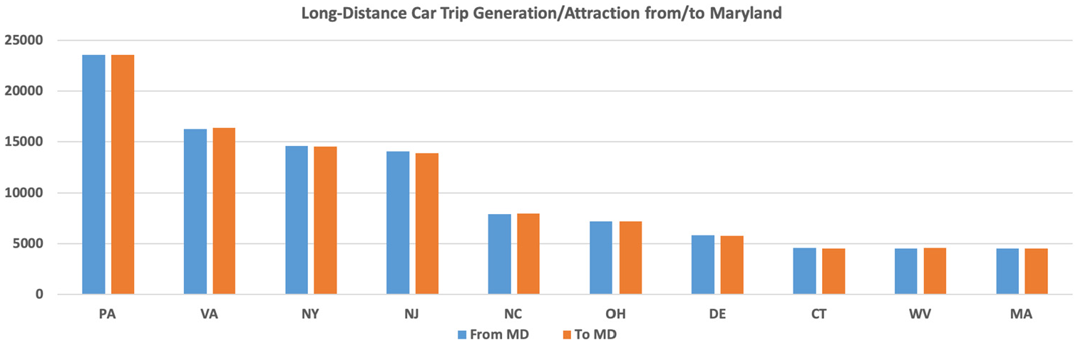
Daily external car trip distribution for Maryland.

Future Year Applications

Scenario Definition

The national long-distance model can be utilized to analyze various policies. To showcase the modeling capabilities, we defined two case study scenarios: a fuel price change scenario and a high-speed rail scenario. The horizon year for both analyses is 2040 and the base year is 2012. Readers can refer to Lu et al. ( 35 ) for more information about the case studies.

Future Year Base Scenario

A realistic assumption for future years is improvement in the fuel economy with new technologies. For the future base scenario, average fuel economy is assumed to increase from 21 mpg to 30 mpg; therefore, OD skim matrices for car trips are altered from the 2012 base year with a cost reduction because of fuel economy change. The train and air OD matrices are assumed to be the same as the 2012 base year.

Scenario 1: Fuel Price Increase

According to projections by U.S. Energy Information Administration (EIA), the price of crude oil in 2040 is expected to increase to around 1.75 times the price in 2012. Therefore, for simplicity, it is assumed that the retail fuel price will also increase accordingly to 1.75 times the 2012 retail fuel price. Since the fuel cost is a smaller proportion of the total operating cost for trains, compared with car and air ( 36 ), it is assumed that the train skim is unchanged. It is worth mentioning that the train level of service usually changes after fuel price variation, but here the effects of the fuel price changes on the railway level-of-service variables are not considered. For car travel, both vehicle economy and fuel price are increased, resulting in different cost changes for different OD pairs based on their distance. The relationship between fuel price change and airfare change is complicated and difficult to forecast, however, it is common knowledge that, given the same number of passengers, the longer the flight distance, the more fuel the airplane will consume. As a reasonable assumption, the airfare is increased by $5.00 if the OD flight distance is less than 500 mi, increased by $10.00 if the distance is between 500 mi and 1000 mi, and increased by $30.00 if the distance is greater than 1000 mi.

Scenario 2: High-Speed Rail

For the second scenario, part of the northeast corridor is selected to forecast the demand for high-speed rail (HSR) and evaluate its impact on the long-distance travel market. With a national-level demand model, it is possible to forecast the future demand for the HSR. However, the research should be conducted on stated preference data since the system has not yet begun. Here, as a proxy for the real HSR, it is assumed that the speed of the current rail system for the Washington, D.C.–New York section of the northeast corridor will be improved in future years and fares will be correspondingly higher. This will certainly affect the travel demand along this corridor. According to Amtrak’s projected planning for construction of HSR in the northeast corridor, the travel time between New York and Washington, D.C., including a stop in Philadelphia, will be reduced to 96 min by 2040. Because of this improvement, the train service costs will be higher accordingly. A 30% increase of travel cost for HSR is used in this scenario.

Data

Similar to the base year case, a synthesized population for the future year is needed. PopGen ( 22 ) is used here as well for generating the population. For the sample data, we used the 2006–2010 ACS five-year PUMS data, and for the marginal data, we used the Complete Economic and Demographic Data Source (CEDDS) by Woods & Poole Economics. After conducting the population synthesis for the entire U.S.A., we selected random states to validate the margins with the CEDDS dataset. The results of the validation were reasonable; therefore PopGen output was used as the input data for simulating the future year population.

Future Year Scenario Results

Given the trip OD tables by purpose, time of year, and travel mode, we can obtain the total number of trips by time of year, travel mode, and purpose. Aggregating all the trips from the trip tables in the base scenario, we can obtain a total of 5.12 billion trips for the year 2040, which means in that year a person would make an average of 12.5 long-distance trips.

Fuel Price Increase

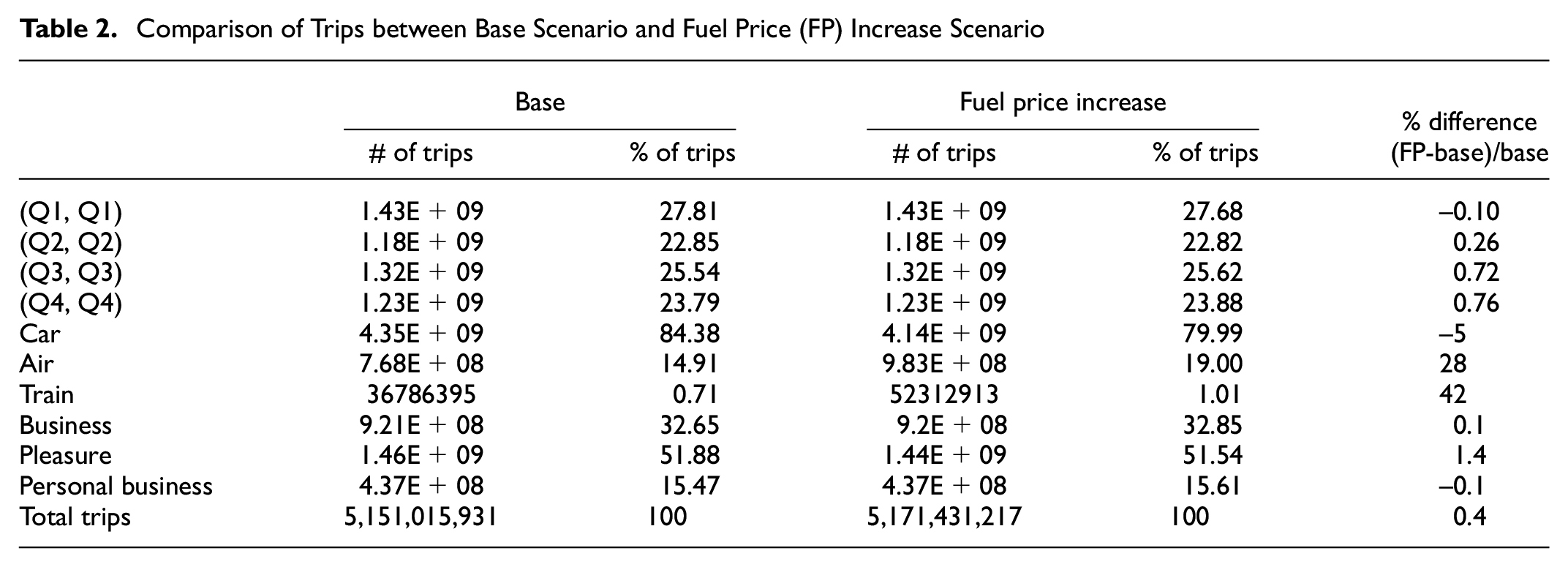
In this scenario, the driving cost increases $ 0.064/mile, which means that making a long-distance trip by car will incur at least $3.20 more (50 mi). The longer distance people travel, the more they pay for their driving cost. The airfare increases $ 0.03/mile at most. Compared with the relatively high base airfare, the increase of the airfare is insignificant. Table 2 presents the numeric comparison of trip count changes for time of year, travel mode, and trip purpose between base scenario and the fuel price increase scenario at the national level. The share of car trips among the total trips at the national level decreases by almost 5% because of the increased driving cost, while the percentage of air and train trips among the total trips increase by 28% and 42%, respectively. Most other changes are small. The significant changes occurred for the number of trips by travel mode, as the fuel price change directly influences the travel mode choice of people undertaking long-distance travel. Fuel cost is an important component of the driving cost. As the travel distance becomes longer, the fuel cost will become more significant. Fuel price increase will increase the driving cost of long-distance travels, which will result in fewer people choosing to travel by car. Compared with fuel cost change for driving and the relatively high airfare, the proposed amount of airfare increase because of the fuel price increase is insignificant. Therefore, travelers have switched to air and train instead of car for long-distance travel. Meanwhile, the cost of travel by train does not change at all, which explains the large change in its share.

Table 2.

Comparison of Trips between Base Scenario and Fuel Price (FP) Increase Scenario

	Base		Fuel price increase		% difference(FP-base)/base
	# of trips	% of trips	# of trips	% of trips
(Q1, Q1)	1.43E+09	27.81	1.43E+09	27.68	−0.10
(Q2, Q2)	1.18E+09	22.85	1.18E+09	22.82	0.26
(Q3, Q3)	1.32E+09	25.54	1.32E+09	25.62	0.72
(Q4, Q4)	1.23E+09	23.79	1.23E+09	23.88	0.76
Car	4.35E+09	84.38	4.14E+09	79.99	−5
Air	7.68E+08	14.91	9.83E+08	19.00	28
Train	36786395	0.71	52312913	1.01	42
Business	9.21E+08	32.65	9.2E+08	32.85	0.1
Pleasure	1.46E+09	51.88	1.44E+09	51.54	1.4
Personal business	4.37E+08	15.47	4.37E+08	15.61	−0.1
Total trips	5,151,015,931	100	5,171,431,217	100	0.4

The results also show that when the fuel price increases, not only does the total number of car trips decrease for all the three income groups, but also the average driving miles per person during one year shrinks for all groups.

High-Speed Rail

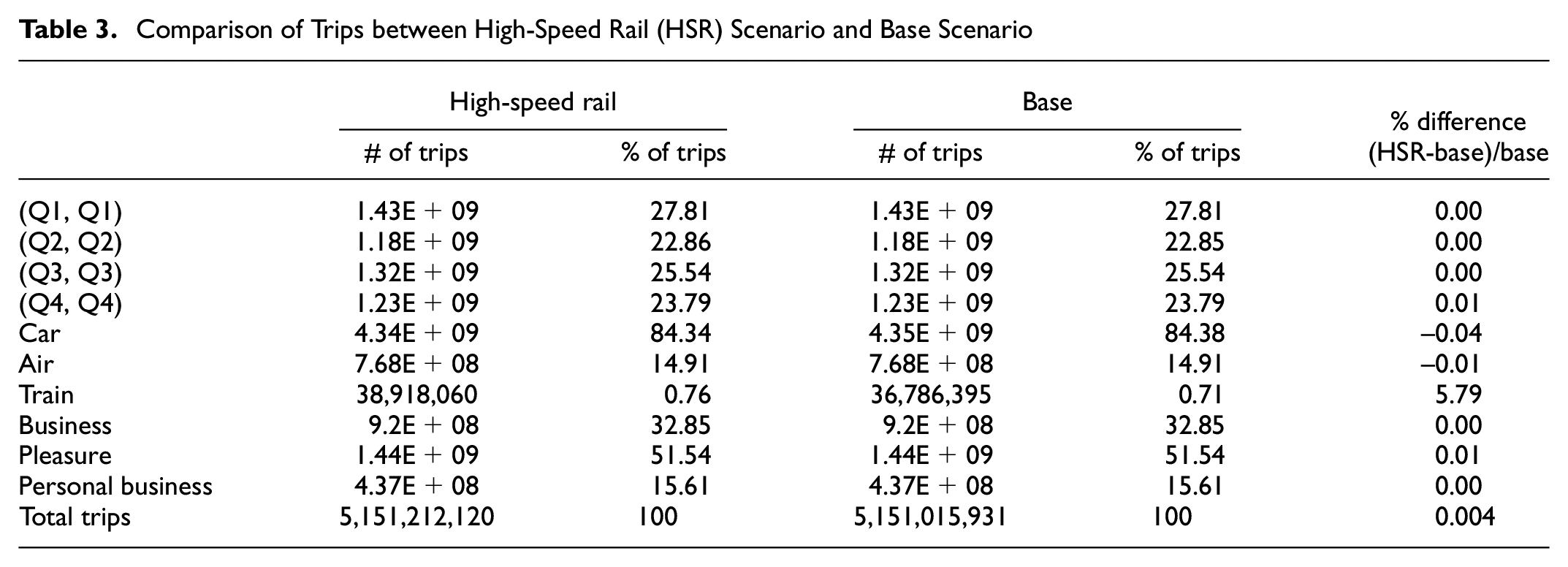
It is expected that with the reduction in travel time of HSR, more people would turn to train for their travel instead of car and air. However, as the train network only covers a limited area, the national mode share for train is not significantly affected. Table 3 summarizes and compares the number of trips for different categories between the HSR scenario and base scenario. The significant change is observed in the number of train trips. Compared with the base scenario, the travel time decrease of the northeast corridor train service increases the total number of train trips by 5.79%, although the HSR is only open for three lines of the northeast corridor. Among all three trip purposes (business, personal business, and pleasure), pleasure travel is affected by HSR the most and represents the largest increase in the number of trips. Business trips follow as the second affected purpose. The HSR has little impact on personal business travel.

Table 3.

Comparison of Trips between High-Speed Rail (HSR) Scenario and Base Scenario

	High-speed rail		Base		% difference(HSR-base)/base
	# of trips	% of trips	# of trips	% of trips
(Q1, Q1)	1.43E+09	27.81	1.43E+09	27.81	0.00
(Q2, Q2)	1.18E+09	22.86	1.18E+09	22.85	0.00
(Q3, Q3)	1.32E+09	25.54	1.32E+09	25.54	0.00
(Q4, Q4)	1.23E+09	23.79	1.23E+09	23.79	0.01
Car	4.34E+09	84.34	4.35E+09	84.38	−0.04
Air	7.68E+08	14.91	7.68E+08	14.91	−0.01
Train	38,918,060	0.76	36,786,395	0.71	5.79
Business	9.2E+08	32.85	9.2E+08	32.85	0.00
Pleasure	1.44E+09	51.54	1.44E+09	51.54	0.01
Personal business	4.37E+08	15.61	4.37E+08	15.61	0.00
Total trips	5,151,212,120	100	5,151,015,931	100	0.004

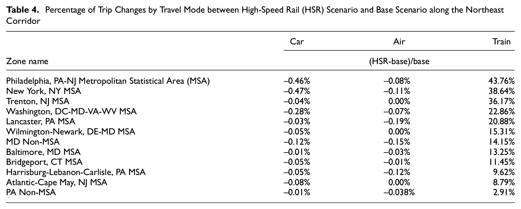
Analyzing the trip changes by travel mode along the northeast corridor shows that the increase in train trips under the HSR scenario is mainly concentrated along the northeast corridor. Table 4 shows the percentage of trip changes by travel mode for zones along the corridor. The largest percentage of increase in number of train trips mainly occurred at stations between Washington D.C. MSA and New York MSA (Philadelphia MSA, Trenton MSA), including D.C. MSA and New York MSA. Philadelphia has the largest percentage of increase in number of train trips (43.76%), because of its location being between the Washington D.C. and New York and its connectivity to multiple rail lines. The train trips from/to New York and Washington D.C. are increased by 38.64% and 22.86% respectively. To the contrary, the number of car trips and air trips of the zones show little change, decreasing by less than 0.5%. Generally, the number of trips by car decreases more than the number of trips by air, which shows that car travel is the main competitor of train travel along this corridor.

Table 4.

Percentage of Trip Changes by Travel Mode between High-Speed Rail (HSR) Scenario and Base Scenario along the Northeast Corridor

	Car	Air	Train
Zone name	(HSR-base)/base
Philadelphia, PA-NJ Metropolitan Statistical Area (MSA)	−0.46%	−0.08%	43.76%
New York, NY MSA	−0.47%	−0.11%	38.64%
Trenton, NJ MSA	−0.04%	0.00%	36.17%
Washington, DC-MD-VA-WV MSA	−0.28%	−0.07%	22.86%
Lancaster, PA MSA	−0.03%	−0.19%	20.88%
Wilmington-Newark, DE-MD MSA	−0.05%	0.00%	15.31%
MD Non-MSA	−0.12%	−0.15%	14.15%
Baltimore, MD MSA	−0.01%	−0.03%	13.25%
Bridgeport, CT MSA	−0.05%	−0.01%	11.45%
Harrisburg-Lebanon-Carlisle, PA MSA	−0.05%	−0.12%	9.62%
Atlantic-Cape May, NJ MSA	−0.08%	0.00%	8.79%
PA Non-MSA	−0.01%	−0.038%	2.91%

The last thing to analyze is the effect of HSR on different groups of people. Table 5 shows the differences in trip counts after the installation of HSR for different population groups. It indicates that the most significant change belongs to the people in income group 3, who change their mode from car to air more than any other group.

Table 5.

Comparison of Percentage of Trips and Trip Changes between High-Speed Rail (HSR) and Base

	Base	HSR	Changes in # of trips
Category	% of trips	% of trips	(HSR trips–base trips)
Inc 1, air	0.84	0.84	−5795
Inc 1, car	5.59	5.59	−87273
Inc 1, train	0.04	0.05	103475
Inc 2, air	4.48	4.48	−21296
Inc 2, car	25.74	25.74	−393541
Inc 2, train	0.22	0.23	465063
Inc 3, air	9.59	9.59	−72507
Inc 3, car	53.04	53.01	−1355064
Inc 3, train	0.45	0.48	1563127
Total	100	100	NA
Male, air	8.86	8.86	−61495
Male, car	44.71	44.69	−902927
Male, train	0.39	0.41	1058576
Female, air	6.05	6.05	−38103
Female, car	39.66	39.64	−932951
Female, train	0.32	0.34	1073089
Total	100	100	NA
Age 1, air	4.47	4.47	−39611
Age 1, car	25.08	25.07	−593362
Age 1, train	0.21	0.23	689245
Age 2, air	6.68	6.68	−37891
Age 2, car	36.55	36.54	−784857
Age 2, train	0.31	0.33	917319
Age 3, air	3.76	3.76	−22096
Age 3, car	22.75	22.74	−457659
Age 3, train	0.19	0.20	525101
Total	100	100	NA

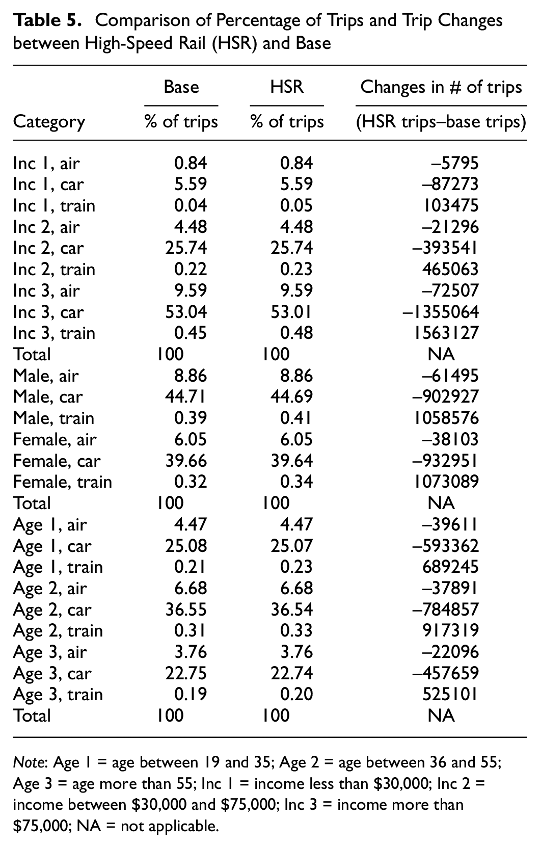
Note: Age 1 = age between 19 and 35; Age 2 = age between 36 and 55; Age 3 = age more than 55; Inc 1 = income less than $30,000; Inc 2 = income between $30,000 and $75,000; Inc 3 = income more than $75,000; NA = not applicable.

Conclusion and Future Research

Studying national long-distance travel requires accurate analysis tools for understanding long-distance travel behavior and forecasting travel patterns in the future, however, analysis of national long-distance passenger travel demand has been an understudied area in transportation planning. This research demonstrates an academic research endeavor on national passenger travel analysis. It aims to provide important insights and to help federal and state agencies with their decision making for corridor-level, regional-level, and national-level infrastructure investment, design, and management projects.

In this research, an integrated tour-based travel demand modeling system was developed for individuals’ quarterly/yearly long-distance or national travel in the U.S.A., at the Metropolitan Statistical Area (MSA)/non-MSA level, which is the finest geographic resolution in the long-distance travel survey data. The model system is developed considering the specific attributes of long-distance travel, such as low frequency, long activity duration, intermediate stops on the tour legs, and different sets of mode alternatives. The modeling system takes into account people’s long-distance travel at both tour level and stop level. Three levels of choice are modeled. The first level is the activity pattern level, which generates the number of different types of activities a person will choose during one year; the second level is the tour level, which contains choices of tour destination, time of year, tour duration, and tour mode; and the third level is the stop-level model system, which includes the number, the purpose, and the location of each intermediate stop made during the inbound and outbound legs of the tour.

Because the model estimation data was not recent, an efficient optimization technique was applied to calibrate the large-scale national travel demand model. The demand model needed to be calibrated with up-to-date data. Because of the complex nature of the model, simulated-based optimization was used. The optimization algorithm needed to require few simulation runs, as each simulation run was very costly; therefore, we used the SPSA algorithm. The model’s mode and time-of-year components were calibrated using DB1B data, and the model’s destination component was calibrated using NHTS 2017. The results of the calibration showed significant improvement of the objective function.

The calibrated model was employed to predict the long-distance travel demand in future years based on a synthetic future year population. Two scenarios, fuel price increase and HSR, in the future year were then analyzed and compared with a base scenario. The comparison showed defendable results. As expected, the results showed that long-distance driving trips are sensitive to change in fuel price. As the fuel price increases, people would decrease their number of car journeys or choose closer locations as the destination of their car trips. For the second scenario, even though the proposed HSR only operated along a selected regional corridor, the total number of national train trips showed an increase of approximately 6%.

This work can be extended with various applications that are of interest to national and regional agencies. Furthermore, the lack of national data for producing national modeling tools can be alleviated with the increasing availability of passively collected mobile device location data. National location data can now be available with a large sample size, a high sighting frequency, and a high location accuracy. Our research team has a plan to take advantage of mobile phone location data, passively collected by mobile devices, to further calibrate the national model.

Footnotes

Author Contributions

The authors confirm contribution to the paper as follows: study conception and design, data collection, and analysis and interpretation of results: Arash Asadabadi, Carlos Carrion, Sepehr Ghader, Yijing Lu, Di Yang and Lei Zhang; draft manuscript preparation: Sepehr Ghader, Yijing Lu, Zhang, and Arash Asadabadi. All authors reviewed the results and approved the final version of the manuscript.

Declaration of Conflicting Interests

The author(s) declared no potential conflicts of interest with respect to the research, authorship, and/or publication of this article.

Funding

The author(s) disclosed receipt of the following financial support for the research, authorship, and/or publication of this article: This research was partly supported by the U.S. Department of Transportation and the National Center for Strategic Transportation Policies, Investments, and Decisions at the University of Maryland.

Any opinions, findings, and conclusions or recommendations expressed in this paper are those of the authors and do not necessarily reflect the views of the sponsors.

References

Lundqvist

Mattsson

L. G.

National Transport Models: Introduction and Comparative Analysis. In National Transport Models. Advances in Spatial Science ( L.

Lundqvist

Mattsson

L. G.

, eds.), Springer, Berlin and Heidelberg, 2002, pp. 1–16.

Aultman-Hall

Harvey

LaMondia

J. J.

Ritter

Design and Response Quality in a One-Year Longitudinal Survey of Overnight and Long-Distance Travel. Transportation Research Procedia, Vol. 11, 2015, pp. 136–153.

Dilger

R. J.

ISTEA: A New Direction for Transportation Policy. Publius: The Journal of Federalism, Vol. 22, No. 3, pp. 67–78.

Gage

R. W.

McDowell

B. D.

ISTEA and the Role of MPOs in the New Transportation Environment: A Midterm Assessment. Publius: The Journal of Federalism, Vol. 25, No. 3, 1995, pp. 133–154.

Cambridge Systematics, Inc. NCHRP Project 08-36, Task 70: National Travel Demand Forecasting Model Phase I Final Scope. National Cooperative Highway Research Program, Transportation Research Board, Washington, D.C., 2008.

Giaimo

G. T.

Schiffer

Transportation Research E-Circular. 2005(E-C075): Statewide Travel Demand Modeling: A Peer Exchange. Longboat Key, FL, 2004.

Urban Land Use and Transportation Center, and HBA Specto Inc. CSTDM09-Model Development: Model Overview. Institute of Transportation Studies, University of California, Davis, 2011.

Erhardt

Freedman

Stryker

Fujioka

Anderson

Ohio Long-Distance Travel Model. Transportation Research Record: Journal of the Transportation Research Board, 2015. 2003: 130–138.

Mishra

Welch

T. F.

Moeckel

Mahapatra

Tadayon

Development of Maryland Statewide Transportation Model and Its Application in Scenario Planning. Presented at 92nd Annual Meeting of the Transportation Research Board, Washington, D.C., 2013.

10.

Ghader

Zhang

Yang

Darzi

Asadabadi

Carrion

Rossi

T. F.

Liu

Mishra

Avner

Rodavuc

Mahapatra

Baber

Integrating Micro-Simulation Models of Short-Distance and Long Distance Trips for Statewide Applications. Presented at 98th Annual Meeting of the Transportation Research Board, Washington, D.C., 2019.

11.

Hamilton

Traffic Forecasting Report–2007. Research Report KTC-08-06/PL 14-07-1F. Kentucky Transportation Center, University of Kentucky, Lexington, 2008.

12.

Horowitz

Creasey

Pendyala

Chen

NCHRP Report 765: Analytical Travel Forecasting Approaches for Project-Level Planning and Design. Transportation Research Board, Washington of the National Acadamies, D.C., 2014.

13.

Outwater

M. L.

Bradley

Ferdous

Bhat

Pendyala

Hess

Daly

LaMondia

Tour-Based National Model System to Forecast Long-Distance Passenger Travel in the United States. Presented at 94th Annual Meeting of the Transportation Research Board, Washington, D.C., 2015.

14.

Outwater

Bradley

Ferdous

Trevino

Lin

Foundational Knowledge to Support a Long-Distance Passenger Travel Demand Modeling Framework: Implementation Report. Federal Highway Administration, McLean, VA, 2015.

15.

Aultman-Hall

Harvey

Sullivan

LaMondia

J. J.

The Implications of Long-Distance Tour Attributes for National Travel Data Collection in the United States. Transportation, Vol. 45, No. 3, 2018, pp. 875–903.

16.

LaMondia

J. J.

Moore

Aultman-Hall

Modeling Intertrip Time Intervals between Individuals’ Overnight Long-Distance Trips. Transportation Research Record: Journal of the Transportation Research Board, 2015. 2495: 23–31.

17.

Sullivan

LaMondia

J. J.

Harvey

Garrison

Aultman-Hall

Analysis of the Long-Distance and Overnight Travel Tour Planning Process. Transportation Research Record: Journal of the Transportation Research Board, 2016. 2594: 1–10.

18.

LaMondia

J. J.

Aultman-Hall

Greene

Long-Distance Work and Leisure Travel Frequencies: Ordered Probit Analysis across Non-Distance-Based Definitions. Transportation Research Record: Journal of the Transportation Research Board, 2014. 2413: 1–12.

19.

Bureau of Transportation Statistics. American Travel Survey. Bureau of Transportation Statistics, U.S. Department of Transportation, Washington, D.C., 1995.

20.

Zhang

Innovative Data Collection and Modeling Methods for Long-Distance Passenger Travel Demand Analysis. UMD-2010-01. U.S. Department of Transportation, Washington, D.C., 2012.

21.

Zhang

US National and Inter-Regional Travel Demand Analysis: Person-Level Microsimulation Model and Application to High-Speed Rail Demand Forecasting. No. Project ID: NTC2014-SU-R-21. National Transportation Center at Maryland, U.S. Department of Transportation, University Transportation Centers Program, 2015.

22.

Konduri

Pendyala

R. M.

Sana

Waddell

A Methodology to Match Distributions of Both Household and Person Attributes in the Generation of Synthetic Populations. Presented at 88th Annual Meeting of the Transportation Research Board, Washington, D.C., 2009.

23.

U.S. Census Bureau. 2000 Census of Population and Housing: Technical Documentation.

24.

Spall

J. C.

An Overview of the Simultaneous Perturbation Method for Efficient Optimization. Johns Hopkins APL Technical Digest, Vol. 19, No. 4, 1998, pp. 482–492.

25.

Spall

J. C.

Introduction to Stochastic Search and Optimization: Estimation, Simulation, and Control. John Wiley & Sons, Hoboken, N.J., 2005.

26.

Spall

J. C.

Multivariate Stochastic Approximation Using a Simultaneous Perturbation Gradient Approximation. IEEE Transactions on Automatic Control, Vol. 37, No. 3, 1992, pp. 332–341.

27.

Dong

Zhang

Calibration of Microsimulation with Heuristic Optimization Methods. Transportation Research Record: Journal of the Transportation Research Board, 2007. 1999: 208–217.

28.

Antoniou

Azevedo

C. L.

Pereira

Ben-Akiva

W–SPSA in Practice: Approximation of Weight Matrices and Calibration of Traffic Simulation Models. Transportation Research Procedia, Vol. 7, 2015, pp. 233–253.

29.

Antoniou

Ben-Akiva

An Enhanced SPSA Algorithm for the Calibration of Dynamic Traffic Assignment Models. Transportation Research Part C: Emerging Technologies, Vol. 51, 2015, pp. 149–166.

30.

Balakrishna

Ben-Akiva

Koutsopoulos

Offline Calibration of Dynamic Traffic Assignment: Simultaneous Demand-and-Supply Estimation. Transportation Research Record: Journal of the Transportation Research Board, 2007. 2003: 50–58.

31.

Tympakianaki

Koutsopoulos

H. N.

Jenelius

c-SPSA: Cluster-Wise Simultaneous Perturbation Stochastic Approximation Algorithm and Its Application to Dynamic Origin–Destination Matrix Estimation. Transportation Research Part C: Emerging Technologies, Vol. 55, 2015, pp. 231–245.

32.

Kattan

Abdulhai

Noniterative Approach to Dynamic Traffic Origin-Destination Estimation with Parallel Evolutionary Algorithms. Transportation Research Record: Journal of the Transportation Research Board. 2006. 1964: 201–210.

33.

Balakrishna

Ganesan

Sherry

Airport Taxi-Out Prediction using Approximate Dynamic Programming: Intelligence-Based Paradigm. Transportation Research Record: Journal of the Transportation Research Board, 2008. 2052: 54–61.

34.

Ghader

Darzi

Carrion

Zhang

Calibration of a Large Scale Travel Demand Model: Microsimulation Model of National Long-Distance Travels. Presented at 98th Annual Meeting of the Transportation Research Board, Washington, D.C., 2019.

35.

Asadabadi

Ghader

Yang

Zhang

National Travel Demand Model for the United States: Applications to Statewide Modeling, Fuel Price, and HSR. Presented at 97th Annual Meeting of the Transportation Research Board, Washington, D.C., 2018.

36.

Tipping

Schmahl

Duiven

Impact of Reduced Oil Prices on the Transportation Sector. Strategy and Business, 2015.