Assessment of the Effects of Volume Completeness and Spatial and Temporal Correlation on Hourly Freeway Crash Prediction Models

Abstract

Traditional traffic safety analyses of crash frequency usually use highly aggregated cross-sectional data and ignore the time-varying nature of some critical factors. This research used 7 years of hourly data from 110 rural four-lane segments and 80 urban six-lane segments to develop hourly level crash prediction models and contrasted them with traditional annual average daily traffic (AADT)-based models. To account for the overdispersion of data and unobserved heterogeneity, generalized linear mixed-effect models were contrasted with negative binomial models. The models used average hourly volume as a measure of exposure, and the quantity of volume data available for the sites ranged from continuous counts to locations where only a couple of weeks of data were available every other year (short counts). While developing disaggregated models, the difference in data availability from these sources can be a potential source of error, so evaluating the change in performance of prediction models with changes in volume data availability was examined. The results showed that the best models include a combination of average hourly volume, selected geometric variables, and speed related parameters. Hourly models that included speed parameters consistently outperformed AADT models. Further investigation revealed that the positive effect of using a more inclusive and larger dataset was larger than the effect of accounting for data correlation. This showed that using short count stations as a data source does not diminish the quality of the developed models, thus indicating that these methods could be applied broadly across agencies, even when volume data is relatively sparse.

The safety performance functions (SPFs) recommended in the Highway Safety Manual (HSM) use annual average daily traffic (AADT) as a measure of exposure ( 1 ). A disadvantage of using AADT in safety analysis is that it does not capture the variation in traffic flow that occurs throughout the day and could mask safety effects of operational changes on a roadway. Flow characteristics such as variation in speed and level of congestion play a significant role in crash occurrence and are not currently accounted for in the HSM.

Previous research by the authors showed that using average hourly volume along with average speed and selected geometric variables from high quality continuous count station data improved predictions compared with models that used AADT and no other traffic state information (2, 3). The researchers also evaluated private sector probe speed data from the vendor INRIX as an alternate source for speed data and concluded that probe speed can be used in lieu of detector speed data without reducing the quality of crash prediction models. These results were based only on continuous count stations that collect high quality volume data but are often widely spaced on state road systems. Most states collect short duration counts (which could range from 2 days to multiple months) on a broader geographic footprint of their roadway network than continuous count data. While these short count stations are much more broadly available, they do not provide as complete a picture of the true average quantity of travel as the continuous count stations.

Given that the prior work showed that crash predictions could be improved by using more disaggregate data at continuous count stations, this paper sought to determine if those trends could extend to short count stations where data availability is more limited, potentially broadening the application of these methods. Additionally, this study incorporates consideration of temporal and spatial variations in the crash prediction models. With hourly data collected from multiple years and from different parts of the state, correlation problems may exist among the records in both the spatial and temporal domains.

Objective

The objectives of this paper are to define the relationship between average hourly crash frequency on freeways and explanatory variables that vary with time and geography. For this paper, data representing crashes that occurred on rural two-lane and urban three-lane freeway directional segments in Virginia were collected for a 7-year period on an hourly level. The volume data used in this study comes from detectors that often did not collect data continuously, so the research sought to determine if positive results previously obtained with continuous count station data were transferable to locations with lower volume data availability ( 3 ). Therefore, evaluating the change in the performance of prediction models with changes in volume data availability and the presence of correlation in data were examined as a way to broaden the applicability of these models.

Literature Review

There has been considerable research conducted in recent years into establishing relationships between crashes and various traffic flow characteristics for freeway segments. Most of the research has focused on determining the relationship between crashes and highway traffic volumes, while little attention has been focused on the relationships of vehicle density, level of service (LOS), volume/capacity (v/c) ratio, and speed distribution (4 –7). Most researchers only focused on selected segments of a particular facility and did not consider the roadway system as a whole while exploring the relationship between crash rates and flow parameters (8 –10). These previous studies relied on data from point detectors, which limits the coverage. In previous research, authors compared different speed data sources and corresponding changes in model quality ( 3 ). It was found that using probe data, which has better network coverage, might be useful to improve the availability and quantity and quality of speed data. Although there has been considerable research in the general direction of safety modeling, paper length limitation prohibits a deeper discussion of past work. A more detailed discussion of past studies can be found in ( 11 ).

While several studies have examined the safety effects of geometric variables (5, 7, 12 –18), the effects of flow state have not traditionally been included in AADT-based crash prediction models. Researchers have found that with an increase in flow, the crash rate initially remains constant until a certain critical threshold combination of speed and density is reached, and then rises rapidly (10, 19 –21). Researchers who developed models using macroscopic or hourly level models also often ignored the correlation that exists in disaggregated data and used generalized linear models (GLM) to develop predictions (4, 22, 23 ). To develop crash risk models at the disaggregated level requires some technical challenges to be overcome, such as correlations by sharing unobserved effects among multiple observations generated from the same road segments, time period, or both (24, 25).

Statistical methods such as random-effects negative binomial models (RENB) that incorporate a panel data structure have gained popularity as a result of their capacity to address both time-series and cross-sectional variations (26, 27). Noland used fixed- and RENB models to investigate the effects of roadway improvements on traffic safety using 14 years of data for all 50 U.S. states ( 28 ). Another study by Li et al. used a mixed-effect negative binomial (MENB) regression model and back-propagation neural network (BPNN) model to consider bus crashes ( 29 ). The MENB model results show that it was advantageous to use a mixed-effects modeling method to predict accident counts because it can take into account the effects of specific factors. Another analysis on urban road segments in Turin, Italy also favored the use of mixed-effect models ( 30 ). Data from 2006 to 2012 were used and traffic flows and weather station data were aggregated in 5-min intervals for 35 min across each crash event. Two different approaches, a BPNN model and a mixed-effect model, were used. The researchers concluded that the mixed model performed well and was also easier to interpret.

Data Collection and Preparation

Volume, speed, and geometry data were collected for two-lane directional rural freeway segments and three-lane directional urban freeway segments from 2011 to 2017 using Virginia Department of Transportation (DOT) data systems. The data were collected on an hourly level and the segments came from different Virginia DOT construction districts.

For this research, only basic freeway segments free from ramps or interchanges were considered. These segments were identified using the detector database maintained by the Virginia DOT Traffic Engineering Division and the Virginia DOT GIS integrator. Using the direction and location information from these databases, segments were identified where there was no entry/exit ramp within 0.5 mi of the start/end of the segment. A segment surrounding each count station was defined such that homogeneous conditions were present for the entire length. If the station was on a link with homogeneous geometric characteristics that was greater than 2 mi in length, a buffer of a maximum 2 mi around the actual location of the detector (1 mi upstream and downstream) was created. The number of lanes, lane and shoulder width, speed limit, median type, and median width were used to define the homogeneity of the segment. Since this research focuses on interaction between geometry and flow parameters and how they define safety instead of a design focused approach, horizontal and vertical curvature was not used to define the segment. Instead they were used as variables to identify their interaction with flow.

Volume Data

A total of 110 count stations were used for rural segments (31 continuous count, 79 short count); for urban segments, the total number of stations was 80 (24 continuous count, 56 short count). The continuous count stations also record speed and usually maintain a high level of data quality. The short count stations are more common, but they do not collect data on a continuous basis and may have a lower level of data quality. For all the continuous count stations, only the periods where volume data meet the quality threshold set by Virginia DOT were included in the dataset. The short count stations collect data periodically, so average volumes were determined using less than an entire year’s worth of data. The average hourly volume data was computed by averaging data for each available hour for each site, so there were always 24 h of data available for each year and each site for the final dataset, even though the number of days used to compute averages varied among sites. AADTs used were taken directly from official Virginia DOT published estimates.

Speed Data

Speed data was obtained from the private sector probe travel time data provider INRIX in hourly intervals. These data are available continuously across the network in real time. Previous research by Dutta and Fontaine evaluated the potential for using speed information from INRIX in combination with continuous count volume data, and validated that INRIX data performed very similarly to the continuous count station speed data ( 3 ). Virginia DOT currently uses INRIX data to support a variety of performance measurement and traveler information applications, and several external and internal evaluations have supported the accuracy of the travel time data for freeways ( 31 ). Similar to the volume data, the average hourly speed was also computed by averaging data for each available hour for each site.

Geometry Data

The Virginia DOT data systems were used to extract geometric and traffic control information such as number of lanes, speed limit, shoulder width, median type, rural/urban designation, and so forth. The vertical curvature (VC) data were collected in the form of percent grade, with positive grades indicating uphill segments and negative grades indicating downhill segments. Horizontal curvature (HC) was expressed using length of the curve, presence of curve as a percentage of segment length, and radius of curve.

Crash Data

Crash data for all the sections were obtained from the Virginia DOT data systems as well. For all the segments, crash information was also collected from 2011 to 2017 inclusive. For this analysis, the researchers examined total crashes as well as fatal and injury crashes. Figure 1 shows the distribution of crashes by site over the study period by year.

Figure 1.

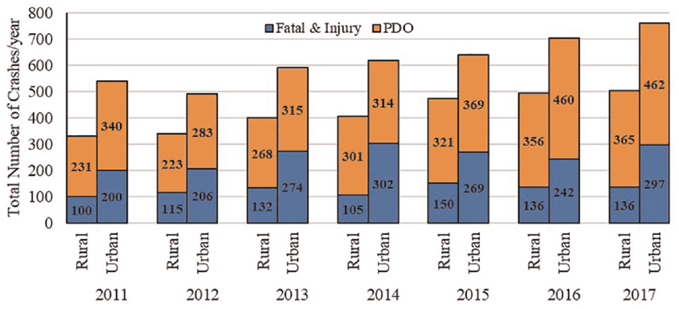
Distribution of total number of crashes for all study segments.

Virginia DOT Districts

Virginia DOT construction districts have been frequently tied with traffic safety variations across the state as a result of differences in driving population, terrain, and traffic conditions. This research used districts as a grouping variable to account for the differences in driving behavior and environment in different parts of Virginia. The Northern Virginia, Fredericksburg, Richmond, and Hampton Roads Districts are predominantly urban, while the remainder of the state is more rural. The Western portion of the state also features mountainous terrain. Figure 2 shows the locations of the districts and the number of study segments on each district. Table 1 summarizes the properties of the study segments.

Table 1.

Descriptive Statistics of Freeway Study Segments

Type of segment	Total mileage (mi)	Variable	Mean	SD	Min.	Max.
Rural four-lane segments (110 segments)	195.07	AADT	18702	6225	4059	34728
		Average hourly volume (vph)	787.30	530.09	12.00	3064.00
		Average hourly speed (mph)	67.83	3.10	48.31	75.72
		Segment length (mi)	1.79	0.29	1.00	2.00
		Lane width (ft)	12.00	0.00	12.00	12.00
		Median shoulder width (ft)	3.93	2.03	0.00	10.00
		Right shoulder width (ft)	5.24	5.08	0.00	12.00
		Median width (ft)	107.8	59.35	4.00	334.00
		Horizontal curvature radius (mile)	2.00	1.58	0.00	5.92
		Horizontal curvature length (mile)	0.76	0.59	0.00	2.00
		Grade (%)	−0.26	0.80	−3.17	1.58
		Speed limit (mph)	69.00	2.64	55.00	70.00
		Annual total cvrashes	5.19	5.13	0	48
		Annual fatal and injury crashes	1.53	1.91	0	19
Urban six-lane segments (80 segments)	125.42	AADT	40731	17667	10931	76207
		Average hourly volume (vph)	1690.71	1186.88	38.75	4960.50
		Average hourly speed (mph)	66.13	3.11	40.46	72.60
		Segment length (mi)	1.60	0.43	0.66	2.00
		Lane width (ft)	12.00	0.00	12.00	12.00
		Median shoulder width (ft)	7.08	3.07	2.00	12.00
		Right shoulder width (ft)	4.88	5.12	0.00	12.00
		Median width (ft)	103.78	86.97	0.00	363
		Horizontal curvature radius (mi)	1.83	1.00	0.00	4.62
		Horizontal curvature length (mi)	0.93	0.53	0.00	2.00
		Grade (%)	−0.29	0.98	−2.69	2.67
		Speed limit (mph)	64.42	4.59	55	70
		Annual total crashes	12.25	11.47	0	81
		Annual fatal and injury crashes	3.31	2.98	0	19

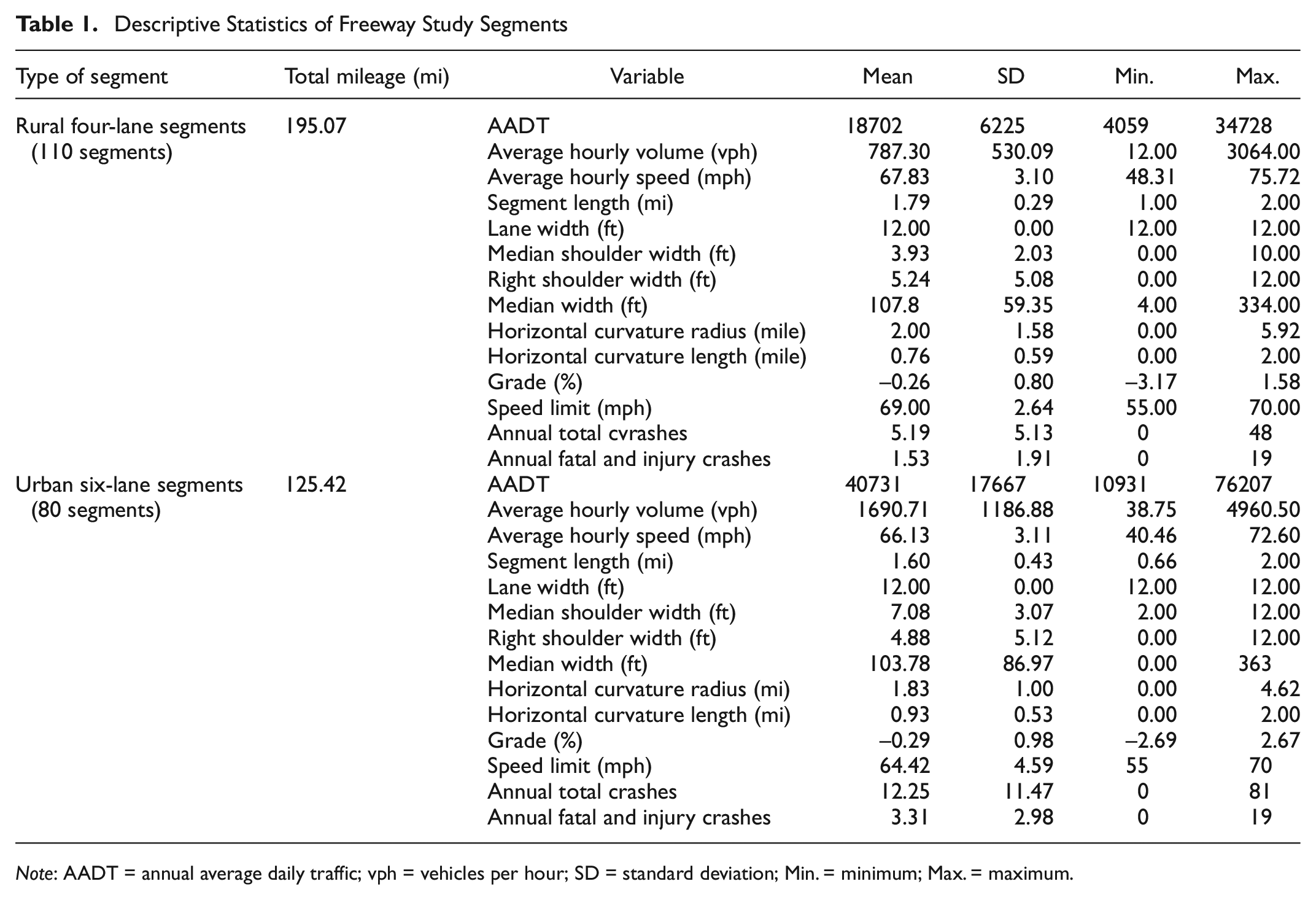
Note: AADT = annual average daily traffic; vph = vehicles per hour; SD = standard deviation; Min. = minimum; Max. = maximum.

Figure 2.

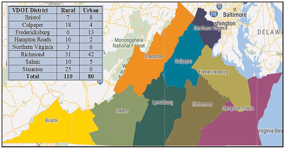
Virginia Department of Transport (VDOT) district map and number of study sites from each district.

Methodology

A series of crash prediction models were developed using a variety of variables related to volume, geometry, and traffic flow parameters. The modeling process started with a simple volume and geometry model and then more complex models were developed by adding traffic variables. Previous research by the authors indicated that when crash prediction models use a data format that is too disaggregated, data errors and imputation of missing values can be problematic and increase errors (2, 3). Based on this previous experience, volumes in this research were expressed as AADT (to be consistent with the current HSM SPFs) and as average hourly volume. To be consistent with the HSM, length was used as an offset variable in the models.

Spatial and Temporal Correlation

Traditionally, most crash frequency models use a cross-sectional data format. Cross-sectional data are observed at a single point of time for several study sites ( 32 ). Since this format overlooks the correlation between crashes and their contributing factors over time, it is not suitable for studies where multiple years of data are available for study sites. Panel data permits identification of variations across individual roadway segments and variations over time. The time-series nature of multiyear data presents serial correlation issues. In a similar vein, there can be correlation over space because roadway entities that are nearby may share unobserved effects.

Negative binomial (NB) regression has become the most common method for developing SPFs and is also the recommended modeling approach in the HSM ( 1 ). The regular NB model, while accounting for overdispersion, will not allow for location-specific effects or serial correlation over time for clustered crash counts. In recent years, mixed-effect models have gained popularity among researchers as a result of their ability to handle both overdispersion and correlation. They are usually called Generalized Linear Mixed Models (GLMM) because they use the common distributions associated with the generalized linear model (GLM) such as Poisson, NB, or zero-inflated models and also account for data structures in which observations cluster within larger groups ( 27 ).

In an NB regression model, the probability of roadway entity i having y_i crashes per time period is defined as:

P (y_{i}) = \frac{\exp (- λ_{i}) * {λ_{i}}^{y_{i}}}{y_{i}!}

(1)

λ_{i} = \exp (β X_{i} + ε_{i})

(2)

where

y_i is the number of crashes for segment i in year t,

β is a vector of the estimable parameters,

X_i is a vector of the explanatory variables, and

exp ( $ε_{i}$ ) is a gamma-distributed error term with mean 1 and variance α ( 33 ).

The addition of this term allows the variance to differ from the mean as:

VAR (y_{i}) = E (y_{i}) [1 + α E (y_{i})] = E (y_{i}) + α E {(y_{i})}^{2}

(3)

Previous work by Dutta and Fontaine investigated the performance of both NB and zero-inflated NB models ( 3 ). Zero-inflated models were never found to provide superior performance to NB models, so they are not discussed in this paper.

The most frequently used modeling technique for crash data is GLMs with NB regression. The multiyear dataset in this study is comprised of multiple rural and urban highway segments and introduces both spatial correlation (data from different districts of Virginia DOT within Virginia) and temporal considerations (average hourly data for 7 years) that a traditional GLM cannot accommodate.

The GLMM model is a regression model of a response variable that contains both fixed and random effects. Fixed-effects terms usually refer to the conventional regression part of the model. Random-effects terms account for variations between groups that might affect the response. The motivation for the random-effects model is that this model can introduce random location-specific or time specific effects into the relationship between the expected numbers of crashes and the covariates of an observation unit i in a given time period t ( 27 ).

The GLMM model structure is:

y_{i} | b \approx Distr [μ_{i}, \frac{σ^{2}}{w_{i}}]

(4)

g (μ) = β X + bZ + δ

(5)

where

$y_{i}$ = dependent variable,

b = random-effects vector,

Distr = a specified conditional distribution of y given b,

µ = the conditional mean of y given b,

$μ_{i}$ is its i-th element,

$σ^{2} =$ the variance or dispersion parameter,

w = the effective observation weight vector ( $w_{i}$ =the weight for observation i),

g(µ) = link function that defines the relationship between the mean response µ and the linear combination of the predictors,

X = fixed-effects design matrix (of independent variables),

β = fixed-effects vector,

Z = random-effects design matrix (of independent variables), and

δ = residuals ( 30 ).

The model for the mean response µ is

μ = g^{- 1} (\hat{η})

(6)

where $g^{- 1} =$ inverse of the link function g(µ), and $\hat{η} = l$ linear predictor of the fixed and random effects of the generalized linear mixed-effects model.

In the simplest term, the mixed-effect model used in this research can be defined as:

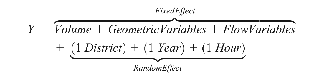
\begin{matrix} Y = \overset{Fixed Effect}{\overset{︷}{Volume + GeometricVariables + FlowVariables}} \\ + \underset{Random Effect}{\underset{︸}{(1 | District) + (1 | Year) + (1 | Hour)}} \end{matrix}

Y is the dependent variable (number of crashes), the fixed effect part defines the relationship between different variables and total crashes, and the random effect part clusters data by Virginia DOT districts (to account for spatial correlation) and by year and hour (to account for temporal correlation). The format “(1|x)” means that the model calculates the variance in intercepts that is different for each group for the random effect “x.” This effectively resolves the non-independence that stems from having multiple responses by the same subject. It is also possible to estimate the random effect for each variable separately. Considering separate parameters for both spatial and temporal effects and for all the correlated variables creates a very complicated model and additional difficulty in interpretation and application. As a result, this paper focuses on the variances between intercepts for each random effect. R statistical software was used for both the GLM and GLMM modeling for this research.

Model Selection and Validation

To measure the model fit, the $ρ_{c}^{2}$ statistic is used based on the log-likelihood of the selected model and the constant-only model:

ρ_{c}^{2} = 1 - \frac{LL (β)}{LL (C)}

(7)

where LL(β) is the log-likelihood at convergence, and LL(C) is the log-likelihood with constant-only model. A perfect model has a likelihood equal to one. The closer the value is to one, the more variance the estimated model is explaining ( 33 ).

A popular method for model selection is the Akaike information criterion (AIC) ( 34 ). AIC offers an estimate of the relative information when a given model is used to represent the process that generated the data. A lower value of AIC indicates a better model. The Bayesian Information Criterion (BIC) is a criterion for model selection among a finite set of models. It is based in part on the likelihood function and it is closely related to the AIC. The BIC also uses a penalty term for the number of parameters in the model. The penalty term is larger in BIC than in AIC ( 35 ).

An objective assessment of the predictive performance of a particular model can be made only through the evaluation of several goodness-of-fit (GOF) criteria. The GOF measures used to conduct external model validation included mean absolute prediction error (MAPE), mean absolute deviation (MAD), and mean squared prediction error (MSPE) ( 33 ). Additionally, cumulative residual (CURE) plots were examined to check the functional form of the model. CURE plots are figures that show how well a model fits the data. When residuals are plotted cumulatively, they demonstrate the suitability of a regression model. The data in the CURE plot are expected to oscillate about 0. Any large jumps between residuals indicate areas where there may be outliers in the data.

Since AADT-based models predict annual crashes while hourly volume models predicted hourly crashes, the summation of hourly predictions was used to generate annual predicted numbers of crashes for the GOF calculations. The average hourly volume data were computed by averaging data for each available hour for each site, so there were always 24 h of data available for each year and each site for validation. Model building used a random selection of 70% of the available data and the remaining 30% was used for testing and validation.

Results and Discussion

The output of GLMM lists some measures of model fit, parameter estimates for the fixed effect part, and the variance between groups for the random effect part. If the variance is indistinguishable from zero, then the correlation within a group is not strong. In the mixed model, one or more random effects are added to the fixed effects. These random effects essentially give structure to the error term “ε.” For this research, random effects for “district,”“year,” and “hour” were considered.

Volume, Length, and Geometry Models

A combination of volume and different geometric variables such as median width, HC, and VC was used to develop initial models. As a result of limited variability in lane width and shoulder width for this particular dataset, they were not found to be significant in the modeling process. Table 2 documents the results from the volume and geometry models.

Table 2.

Parameter Estimates for Volume and Geometry Models for Rural and Urban Segments

Urban/rural	Rural								Urban
Crash severity	Total				Injury				Total				Injury
Volume level	Avg. hour		AADT		Avg. hour		AADT		Avg. hour		AADT		Avg. hour		AADT
Fixed effect	Est.	p-value	Est.	p-value	Est.	p-value	Est.	p-value	Est.	p-value	Est.	p-value	Est.	p-value	Est.	p-value
Intercept	−7.04	<0.01	−9.98	<0.01	−7.13	<0.01	−11.8	<0.01	−6.68	<0.01	−5.55	<0.01	−8.62	<0.01	−7.75	<0.01
log (volume)	0.67	<0.01	1.11	<0.01	0.54	<0.01	0.67	<0.01	0.67	<0.01	0.65	<0.01	0.71	<0.01	0.71	<0.01
Horizontal curve radius (mi)	−0.05	0.01	na	na	na	na	na	na	−0.09	<0.01	−0.14	<0.01	−0.12	0.02	na	na
Median width (ft)	0.21	<0.01	na	na	0.14	<0.01	na	na	na	na	na	na	na	na	na	na
% of Horizontal curve length
<25%	0.53	<0.01	0.28	0.01	na	na	na	na	na	na	na	na	na	na	na	na
>25% to ≤50%	0.24	0.01	0.13	<0.01	na	na	na	na	na	na	na	na	na	na	na	na
>50% to ≤75%	0.46	<0.01	0.27	0.01	na	na	na	na	na	na	na	na	na	na	na	na
>75%	0.09	0.34	0.16	0.87	na	na	na	na	na	na	na	na	na	na	na	na
Length of horizontal curve (mi)
≤0.5	na	na	na	na	na	na	na	na	0.04	0.81	0.26	<0.01	0.94	0.02	0.72	<0.01
>0.5 to ≤1.0	na	na	na	na	na	na	na	na	0.45	0.01	0.60	<0.01	1.32	<0.01	0.93	<0.01
>1.0 to ≤1.5	na	na	na	na	na	na	na	na	0.61	<0.01	0.94	<0.01	1.46	<0.01	1.15	<0.01
>1.5	na	na	na	na	na	na	na	na	0.26	0.2	0.44	<0.01	1.13	<0.01	0.81	<0.01
Grade
Positive grade	na	na	na	na	na	na	na	na	−0.04	0.40	na	na	na	na	na	na
Negative grade	na	na	na	na	na	na	na	na	0.22	<0.01	na	na	na	na	na	na
Random effect (intercept [standard deviation])
District	0.182 (0.047)		0.198 (0.028)		0.132 (0.055)		0.065 (0.048)		0.129 (0.071)		0.173 (0.054)		0.132 (0.053)		0.137 (0.256)
Year	0.465 (0.105)		0.317 (0.049)		0.297 (0.017)		0.193 (0.025)		0.576 (0.087)		0.215 (0.083)		0.242 (0.085)		0.267 (0.032)
Hour	0.538 (0.241)		na		0.419 (0.047)		na		0.618 (0.145)		na		0.529 (0.057)		na
AIC	10782.9		2324.3		4777.3		1485		10217.9		1538		4600.3		1015.5
BIC	10870.1		2361.3		4828.2		1505.5		10311.7		1576.8		4687.4		1054.2
$ρ_{c}^{2}$	0.21		0.19		0.11		0.07		0.15		0.10		0.14		0.10

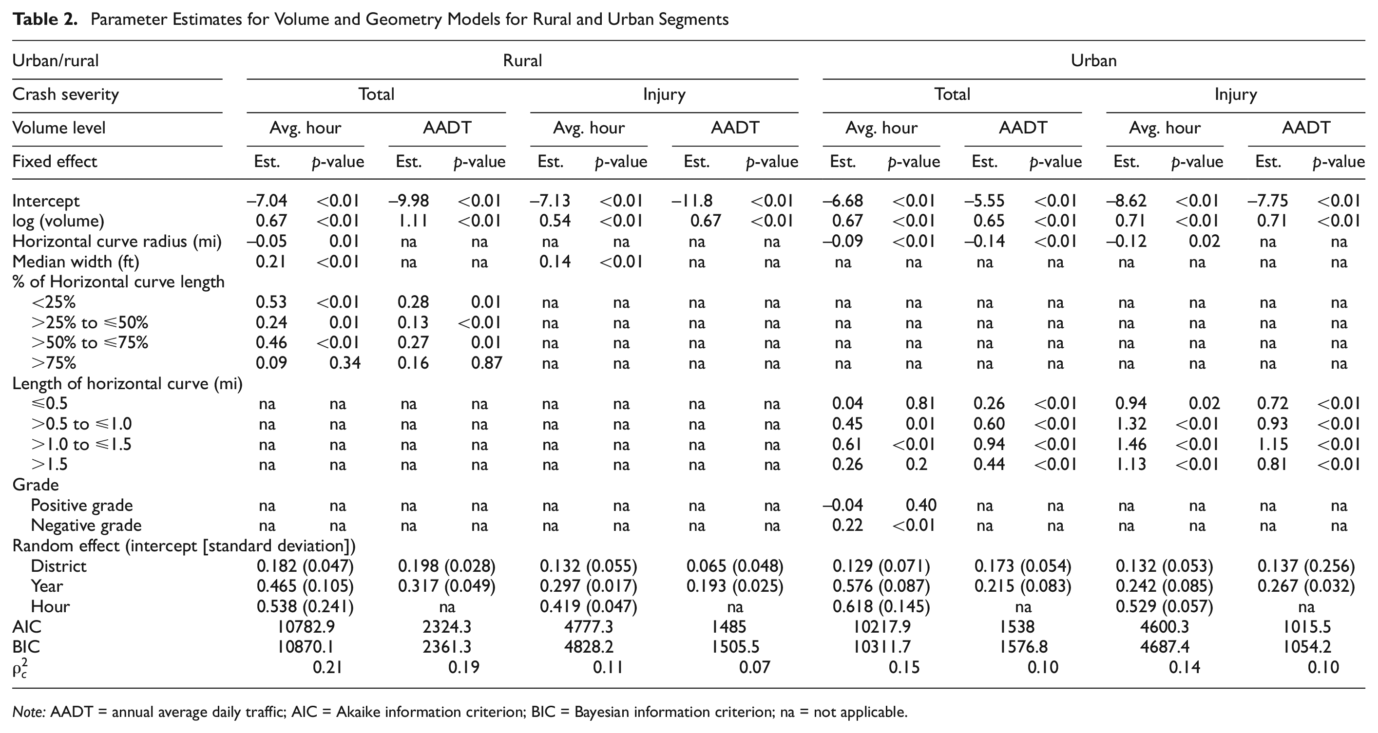
Note: AADT = annual average daily traffic; AIC = Akaike information criterion; BIC = Bayesian information criterion; na = not applicable.

For urban segments, median width, radius and length of HC, and grade were significant variables. For total and injury crashes, the radius of the HC was negatively associated with crash frequency. A larger radius indicates a flatter curve, so this relationship is intuitive. Similarly, increases in the length of the HC increase the probability of a crash. This finding is also consistent with previous research (5, 6). Only negative vertical grades had a statistically significant relationship. Since speed usually increases while driving downhill, this finding is logical. Median width indicated that wider medians in urban segments reduce the total number of crashes. Previous research indicated that median widths between 20 and 30 ft generally show a mixed effect on crashes and median widths of 60 to 80 ft have decreasing effect on crashes (17, 36). About 65% of the urban dataset had median widths within this range, so the negative relationship between median width and crashes is intuitive.

For rural segments, 71% of the data came from segments with median widths greater than 80 ft and no median barrier. The results indicated that wider medians generally had more crashes. This is contradictory to the urban segments, but consistent with previous research (18, 37). The relationship between median width and crashes largely depends on the type of facility, crash type, and also presence and type of a median barrier. Cross median crashes tend to decrease with increasing median width, whereas rollover crashes tend to increase. The radius of the HC had a similar relationship as urban segments where crashes decrease with an increase in the curve radius. The presence of an HC as a percent of total segment length had a more significant effect on total crashes than length of curve.

Volume, Geometry, and Flow Parameter Models

The next set of models was created by adding flow parameters to the models selected in the previous step. Average speed, standard deviation of speed, and the difference between speed limit and average speed (called the delta speed hereafter) were selected to represent traffic flow. If the delta speed is negative, average speed is higher than the speed limit, meaning a free flow condition exists (represented by Delta 1 in models). When this value is positive, speed limit is higher than average speed, meaning the segment is congested (represented by Delta 2 in models). AADT-based models were not developed for this alternative since average speed over a year showed little variability. Table 3 shows both the rural and urban models that include speed parameters.

Table 3.

Parameter Estimates for Volume, Geometry, and Flow Based Models for Rural and Urban Segments

Rural segments					Urban segments
	Total crashes		Injury crashes			Total crashes		Injury crashes
Fixed effect	Estimate	Pr(>\|z\|)	Estimate	Pr(>\|z\|)	Fixed effect	Estimate	Pr(>\|z\|)	Estimate	Pr(>\|z\|)
Intercept	−8.61	<2e-16	−6.73	<2e-16	Intercept	−5.8	<2e-16	−6.79	<2e-16
log (volume)	0.54	1.50E-12	0.41	4.00E-14	log (volume)	0.44	<2e-16	0.37	3.90E-11
Radius of horizontal curve (mi)	−0.06	0.00443	na	na	Radius of horizontal curve (mi)	−0.08	0.00563	−0.09	0.00408
% of horizontal curve length					Length of horizontal curve
Less than 25%	0.53	6.60E-07	na	na	≤0.5	0.76	1.40E-05	0.89	0.00013
>25% ~≤50%	0.11	0.000025	na	na	>0.5 ~≤1.0	1.06	6.40E-10	1.2	1.50E-07
>50% ~≤75%	0.41	1.20E-05	na	na	>1.0 ~≤1.5	1.16	3.60E-11	1.34	4.40E-08
>75%	0.13	0.19522	na	na	>1.5	0.75	2.10E-05	0.85	0.00034
Speed	0.03	0.00974	na	na
Standard deviation	0.17	<2e-16	0.16	2.00E-11	Standard deviation	0.11	<2e-16	0.12	<2e-16
Delta					Delta
Delta 1	0.31	9.05E-06	1.29	<2e-16	Delta 1	0.14	2.10E-04	0.98	<2e-16
Delta 2	0.04	0.57048	−0.29	0.0014	Delta 2	0.03	0.58262	−0.21	0.00438
Random effect	Intercept (standard deviation)		Intercept (standard deviation)		Random effect	Intercept (standard deviation)		Intercept (standard deviation)
District	0.182 (0.017)		0.174 (0.035)		District	0.137 (0.007)		0.152 (0.022)
Year	0.212 (0.045)		0.111 (0.013)		Year	0.326 (0.181)		0.254 (0.159)
Hour	0.508 (0.003)		0.263 (0.092)		Hour	0.546 (0.032)		0.324 (0.092)
AIC	10679		5716.8		AIC	10185.9		6025.2
BIC	10795.1		5782.1		BIC	10293.1		6119.2
$ρ_{c}^{2}$	0.29		0.18		$ρ_{c}^{2}$	0.23		–0.24

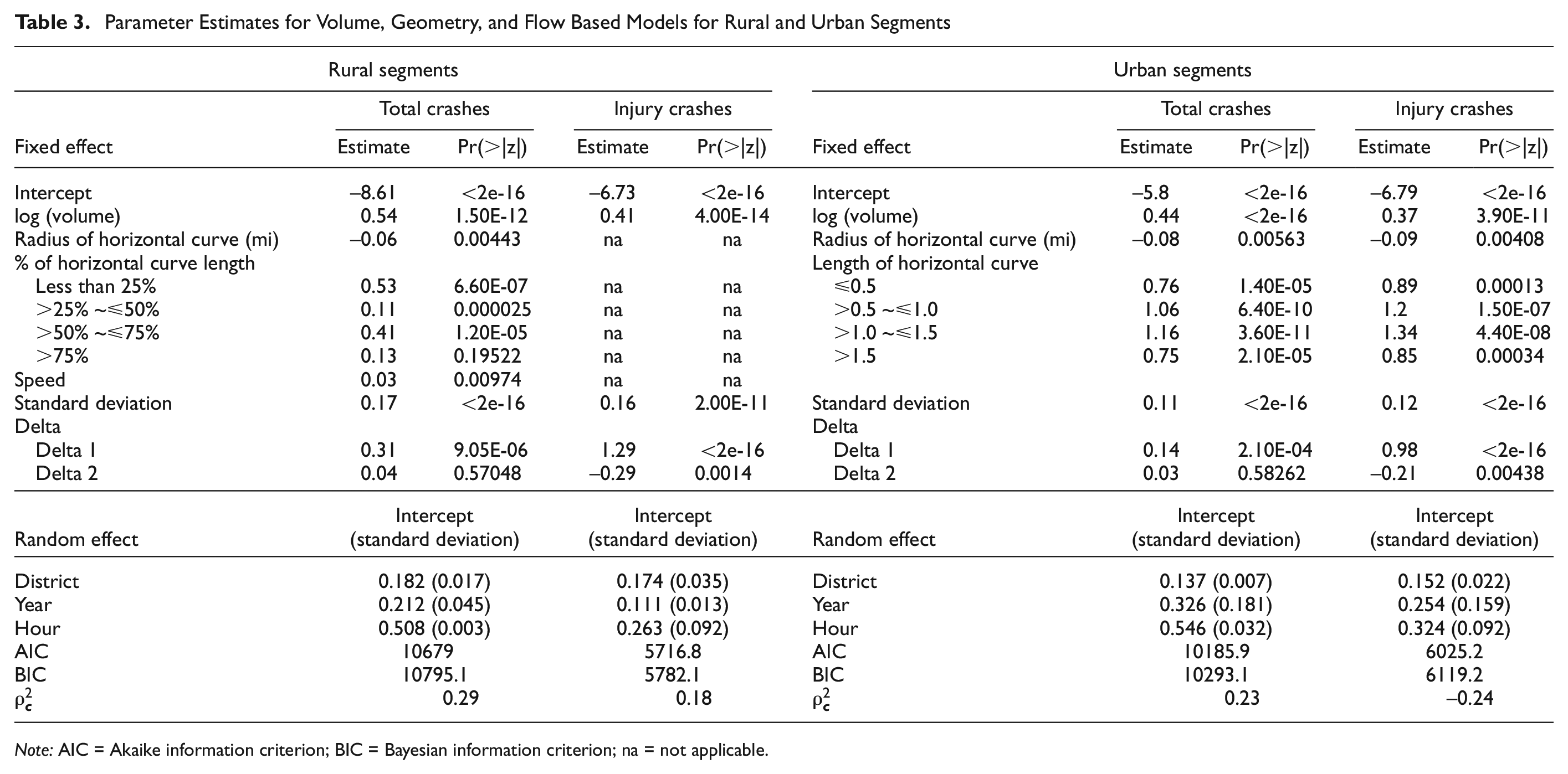
Note: AIC = Akaike information criterion; BIC = Bayesian information criterion; na = not applicable.

For rural segments, average hourly speed was positively related to total crashes, meaning that higher average speed is correlated with higher crash frequency. Standard deviation of speed was significant for all crash types and indicated that as more variation in hourly speeds is observed over a year, the frequency of crashes increases. The variable delta that represents the difference between speed limit and average speed was significant for all crash types as well. It was observed that injury crashes increase during free flow conditions (Delta 1) and decrease during congestion (Delta 2). This is a logical relationship given the relative velocities during collision. The speed parameters showed consistent results for urban segments as well. Standard deviation of average speed always had an increasing effect on crash frequency for all crash types. During free flow conditions (Delta 1), total crashes and injury crashes increase. This relationship is intuitive and consistent with rural segments.

Figure 3 shows the CURE plots for average hourly volume from the volume, flow, and geometry models. CURE plots are not only a reflection of the functional form of the explanatory variable, but also whether other relevant explanatory factors have been included in the model in an appropriate form. Figure 3 shows that for both rural and urban segments, the CURE plots for hourly volume are within the limit of 2 standard deviations. This reinforces the suitability of volume, flow, and geometry models and also shows that the inclusion of volume in the average hourly level form is appropriate.

Figure 3.

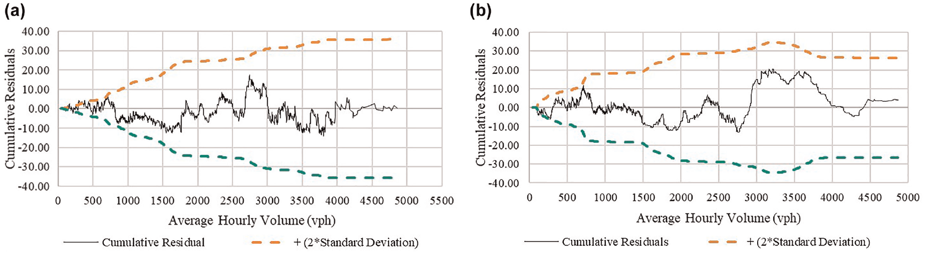
Hourly volume cumulative residual (CURE) plots for: (a) rural segments; and (b) urban segments.

Effect of Correlation

The spatial correlation in the data was represented by the “District” variable. For all models, the intercept and standard deviation for this group revealed that even though a correlation was present between segments that belong to the same district, in general, the spatial correlation was weaker than the temporal one. For all categories, the variance was much smaller for districts than it was for year or hour. This is as a result of an unequal distribution of sample size among districts, as seen in Figure 1. A larger dataset where all the districts are equally represented could shed more light on the spatial correlation. The temporal correlation was modeled using year and hour since the dataset consists of hourly data for 7 years. For both urban and rural models, the temporal correlation was stronger than the spatial one, but still the variance in data explained by yearly correlation was smaller than the hourly one. The total crashes varied between years and total sample size while considering hourly correlation was higher as well. Having more segments in both rural and urban categories could produce a model where stronger temporal correlations have been defined.

Model Comparison

Comparison between Mixed-Effect (GLMM) Models

Table 4 shows the comparison of performance among the models developed. For the rural hourly volume, geometry, and flow models, MAD, MAPE, and MSPE improved by 64%, 26%, and 62% respectively for total crashes and by 39%, 20%, and 40% respectively for injury crashes as compared with AADT models. For the urban models, similar trends were observed where MAD, MAPE, and MSPE improved by 51%, 18%, and 53% respectively for total crashes and by 45%, 18%, and 59% for injury crashes as compared with AADT models. Since the AADT models did not include speed as a variable, for comparison purposes, the volume, flow, and geometry model were compared with the AADT-based volume and geometry models.

Table 4.

Model Comparisons

	Total crashes
	Average hourly volume			AADT
Rural segments	MAD	MAPE	MSPE	MAD	MAPE	MSPE
Volume, length, and geometry models^*	1.16 (–63%)	55% (–14%)	2.92 (–57%)	3.1	69%	6.87
Volume, length, geometry, and flow state models^**	1.11 (–64%)	43% (–26%)	2.59 (–62%)	na	na	na
	FI crashes
	Average hourly volume			AADT
	MAD	MAPE	MSPE	MAD	MAPE	MSPE
Volume, length, and geometry models^*	0.73 (–33%)	33% (–15%)	1.58 (–32%)	1.09	48%	2.33
Volume, length, geometry, and flow state models^**	0.66 (–39%)	28% (–20%)	1.39 (–40%)	na	na	na
	Total crashes
	Average hourly volume			AADT
Urban segments	MAD	MAPE	MSPE	MAD	MAPE	MSPE
Volume, length, and geometry models^*	1.92 (–36%)	35% (–12%)	47.92 (–40%)	2.98	47%	79.43
Volume, length, geometry, and flow state models^**	1.45 (–51%)	29% (–18%)	36.95 (–53%)	na	na	na
	FI crashes
	Average hourly volume			AADT
	MAD	MAPE	MSPE	MAD	MAPE	MSPE
Volume, length, and geometry models^*	1.09 (–36%)	12% (–14%)	4.58 (–48%)	1.69	26%	8.82
Volume, length, geometry, and flow state models^**	0.93 (–45%)	8% (–18%)	3.63 (–59%)	na	na	na

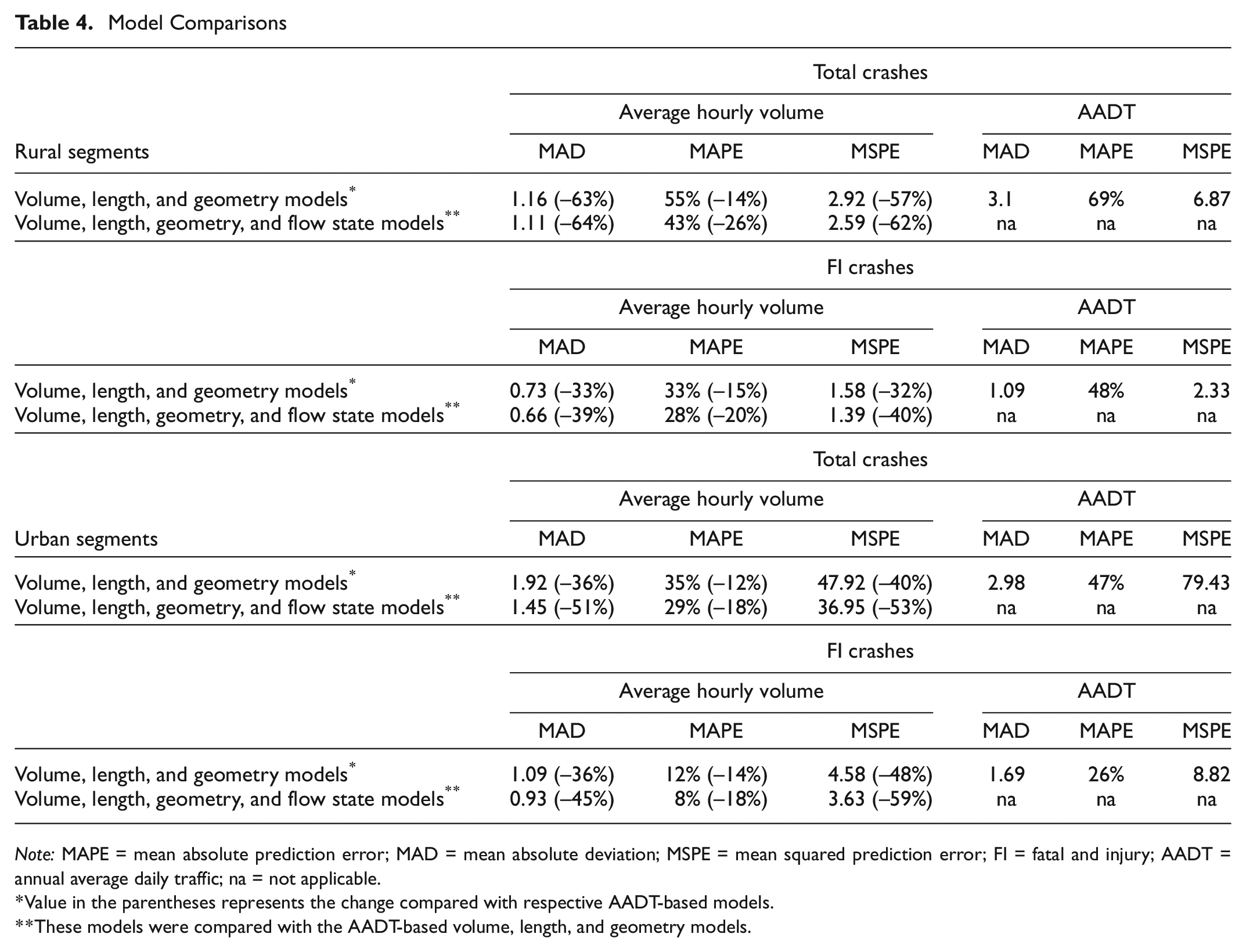
Note: MAPE = mean absolute prediction error; MAD = mean absolute deviation; MSPE = mean squared prediction error; FI = fatal and injury; AADT = annual average daily traffic; na = not applicable.

Value in the parentheses represents the change compared with respective AADT-based models.

These models were compared with the AADT-based volume, length, and geometry models.

The comparison results reinforce the importance of selecting an appropriate disaggregation level. Aggregated models that rely on AADT may fail to capture variations in traffic flow that could influence safety. Hourly aggregation showed better performance compared with the AADT models. Another very important finding was that speed variables played a significant role in model performance. Currently, traffic volume is widely used as a measure of exposure. The same traffic flow occurring on road sections with different capacities creates different operating conditions, and, therefore, different probabilities for crashes. Since current models only rely on volume, the quality of volume data dictates the quality of model. This research showed that speed data from INRIX coupled with volume data with mixed data quality can significantly improve model performance compared with AADT models.

Effects of Correlation and Volume Source

All the models discussed in the prior section were developed using GLMM, so the relative performance quantifies the effect of data aggregation and variable selection. The model comparison in the previous section showed that the best models for this dataset were the volume, geometry, and flow models. Similar results were found when researchers compared continuous count station models without any data correlation ( 3 ).

To isolate the effects of using the broader dataset comprised of continuous count stations and short count stations and the effect of correlation, three types of volume, geometry, and flow model were compared. Model 1 was developed using only continuous count station data and NB regression, taken from previous research ( 3 ). Model 3 was developed in this paper using a combination of short and continuous count data and mixed-effect GLM. Model 2 was developed by re-running model 3 without considering any correlation. This model used data from model 3 and NB regression from model 1. A comparison of all three models is shown in Table 5 based on total crashes.

Table 5.

Model Comparison to Check for Data Quality and Correlation

	Rural segments
	Data source	Total segments	Correlation	MAD	MAPE	MSPE
Model 1	Continuous count only	31 rural segments, 23 urban segments	No	3.24	48%	23.5
Model 1	Continuous count only	31 rural segments, 23 urban segments	No	na	na	na
Model 2	Continuous and short count	110 rural segments, 80 urban segments	No	1.56	44%	6.63
Model 2	Continuous and short count	110 rural segments, 80 urban segments	No	(–52%)	(–4%)	(–72%)
Model 3	Continuous and short count	110 rural segments, 80 urban segments	Yes	1.11	43%	2.59
Model 3	Continuous and short count	110 rural segments, 80 urban segments	Yes	(–66%)	(–5%)	(–89%)
	Urban segments
	Data source	Total segments	Correlation	MAD	MAPE	MSPE
Model 1	Continuous count only	31 rural segments, 23 urban segments	No	6.82	33%	124.35
Model 1	Continuous count only	31 rural segments, 23 urban segments	No	na	na	na
Model 2	Continuous and short count	110 rural segments, 80 urban segments	No	2.89	30%	60.54
Model 2	Continuous and short count	110 rural segments, 80 urban segments	No	(–58%)	(–3%)	(–51%)
Model 3	Continuous and short count	110 rural segments, 80 urban segments	Yes	1.45	29%	36.95
Model 3	Continuous and short count	110 rural segments, 80 urban segments	Yes	(–79%)	(–4%)	(–70%)

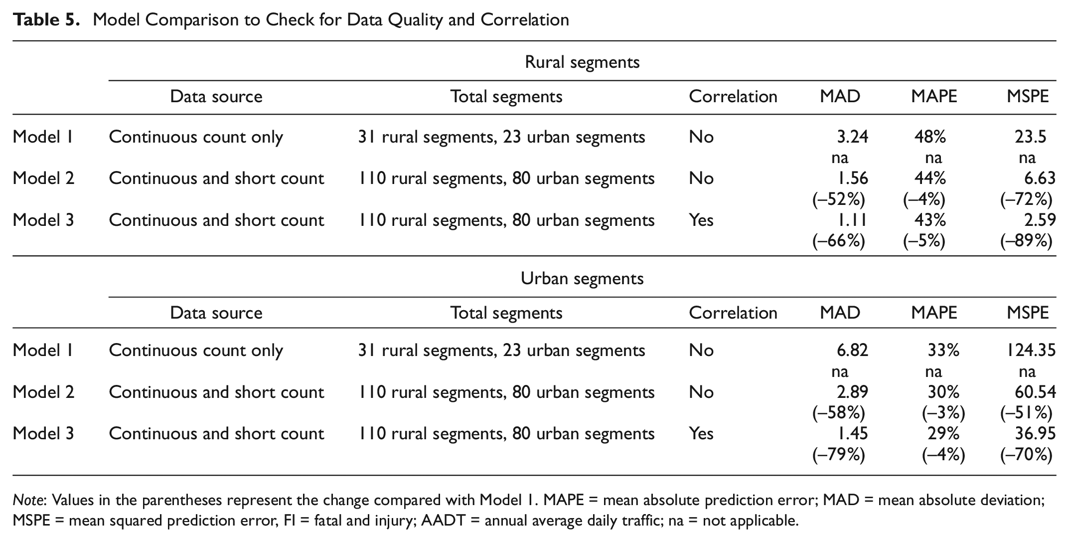
Note: Values in the parentheses represent the change compared with Model 1. MAPE = mean absolute prediction error; MAD = mean absolute deviation; MSPE = mean squared prediction error, FI = fatal and injury; AADT = annual average daily traffic; na = not applicable.

The results show that for both rural and urban segments, the inclusion of the short count stations in Model 2 had a large beneficial effect on model performance compared with Model 1. Acknowledging data correlation also had a positive effect as seen on Measures of Effectiveness (MOEs) for Model 3, although the incremental improvement was lower than that from the inclusion of the short count stations. For rural hourly models, MAD, MAPE, and MSPE improved by 52%, 4%, and 72% respectively for Model 2 in comparison to Model 1. The improvement in model performance can be attributed to the size of the dataset. The MAD, MAPE, and MSPE further improved by 66%, 5%, and 89% between Model 1 and Model 3. The improved performance for model 3 was as a result of the more appropriate methodology acknowledging correlation and also using a broader dataset. The urban segments showed similar results as well.

Since current models only rely on volume, the quality of volume data dictates the quality of the model. The larger effect of using an extensive dataset proved that using short count stations as a data source does not diminish the quality of developed models if continuous speed related variables are used in the model. This means that a combination of a lower quality volume data source with good quality speed data can lessen the dependency on volume data quality without compromising performance. Since short count stations are more common, this finding also ensures making the best use of available resources in future research and application.

Conclusion

The models that include speed-related variables in combination with volume and geometry provided superior predictions to ones that did not include speed variables. The average hourly models open up the possibility of more accurate safety assessment of facilities with dynamic traffic control or geometry. The current practice of using AADT-based SPFs cannot capture the dynamic safety effects of work zones, part time hard shoulder running, variable speed limits, or other operational treatments that have varying effects throughout the day. The models in this paper would improve the safety analysis of these countermeasures.

The essential requirement for establishing a relationship between crashes and flow state on a disaggregate level is reliable information on crashes, hourly traffic flow data, and geometric factors. This type of analysis has not been done previously because obtaining reliable data about crashes and traffic flow states is not a trivial task. Adequate detector coverage and quality of available data is a major issue in most states, making it difficult to acquire widespread information on quality of flow. From that perspective, this research sheds light on using various data sources to create a dataset of mixed quality volume data and good quality speed data.

The random effect part of the modeling showed that the spatial correlations between districts were weaker than the temporal correlations. The variances in data between years and hours were small as well. This finding was reinforced during model validation where having a broader and more inclusive dataset (regardless of continuous volume data availability) had a greater effect than data correlation.

This research can be extended to develop disaggregated models for other facility types. Comparing different statistical methodologies to address correlation and different nesting structures among variables can also be useful. Another potential area for future research could be to explore different ways of defining congestion and its effect on model performance.

Footnotes

Author Contributions

The authors confirm contribution to the paper as follows: study conception and design: Nancy Dutta, Michael Fontaine; data collection: Nancy Dutta; analysis and interpretation of results: Nancy Dutta; draft manuscript preparation: Nancy Dutta, Michael Fontaine. All authors reviewed the results and approved the final version of the manuscript.

Declaration of Conflicting Interests

The author(s) declared no potential conflicts of interest with respect to the research, authorship, and/or publication of this article.

Funding

The author(s) received no financial support for the research, authorship, and/or publication of this article.

References

Highway Safety Manual , 1st ed. American Association of State Highway Transportation Officials. Washington, D.C., 2010.

Dutta

Fontaine

Developing Rural Four Lane Freeway Crash Prediction Models using Hourly Flow Parameters. IATSS Research, 2019. (Under Review).

Dutta

Fontaine

Improving Freeway Segment Crash Prediction Models By Including Disaggregate Speed Data from Different Sources. Accident Analysis and Prevention, Vol. 132, 2019. https://doi.org/10.1016/j.aap.

Ivan

J. N.

Wang

Bernardo

N. R.

Explaining Two-Lane Highway Crash Rates using Land Use and Hourly Exposure. Accident Analysis and Prevention, Vol. 32, 2000, pp. 787–795.

Khan

Bill

Chitturi

Noyce

Safety Evaluation of Horizontal Curves on Rural Undivided Roads. Transportation Research Record: Journal of the Transportation Research Board, 2013. 2386: 147–157.

Zegeer

Stewart

Reinfurt

Council

Neuman

Hamilton

Miller

Hunter

Cost Effective Geometric Improvements for Safety Upgrading of Horizontal Curves. FHWA/RD-90-021. Federal Highway Administration, McLean, VA, 1990.

Shankar

Mannering

Barfield

Effect of Roadway Geometrics and Environmental Factors on Rural Freeway Accident Frequencies. Accident Analysis and Prevention, Vol. 27, No. 3, 1995, pp. 371–389.

Kononov

Lyon

Allery

Relation of Flow, Speed, and Density of Urban Freeways to Functional form of a Safety Performance Function. Transportation Research Record: Journal of the Transportation Research Board, 2011. 2236: 11–19.

Zhou

Sisiopiku

Relationship Between Volume-to-Capacity Ratios and Accident Rates. Transportation Research Record: Journal of the Transportation Research Board, 1997. 1581: 47–52.

10.

Imprialou

M. I. M.

Quddus

Pitfield

D. E.

Lord

Re-Visiting Crash-Speed Relationships: A New Perspective in Crash Modelling. Accident Analysis and Prevention, Vol. 86, 2016, pp. 173–185.

11.

Dutta

Fontaine

M. D.

Improving Freeway Crash Prediction Models using Disaggregate Flow State Information. FHWA/VTRC 20-R15. Virginia Transportation Research Council, 2020.

12.

Tegge

R. A.

J. H.

Ouyang

Development and Application of Safety Performance Functions for Illinois. ICT-R27-20. Illinois Center of Transportation, 2010.

13.

Miaou

The Relationship between Truck Accidents and Geometric Design of Road Sections: Poisson versus Negative Binomial Regression. Accident Analysis and Prevention, Vol. 26, No. 4, 1994, pp. 471–482.

14.

Jianming

Kockelman

Crash Frequency and Severity Modeling Using Clustered Data from Washington State. Proc., IEEE Intelligent Transportation Systems Conference, Toronto, Canada, 2006.

15.

Milton

J. C.

Mannering

F. L.

The Relationship between Highway Geometrics, Traffic Related Elements and Motor Vehicle Accidents.WA-RD 403.1. Washington State Department of Transportation, 1996.

16.

Geedipally

S. R.

Pratt

M. P.

Lord

Effects of Geometry and Pavement Friction on Horizontal Curve Crash Frequency. Journal of Transportation Safety & Security, 2017. https://doi.org/10.1080/19439962.2017.1365317.

17.

Knuiman

Council

Reinfurt

Association of Median Width and Highway Accident Rates. Transportation Research Record: Journal of the Transportation Research Board, 1993. 1401: 70–82.

18.

Graham

J. L.

Harwood

D. W.

O’Laughlin

M. K.

Donnell

E. T.

Brennan

NCHRP Report 794: Median Cross-Section Design for Rural Divided Highways. Transportation Research Board of the National Academies, 2014.

19.

Kononov

Hersey

Reeves

Allery

Relationship Between Freeway Flow Parameters and Safety and Its Implications for Hard Shoulder Running. Transportation Research Record: Journal of the Transportation Research Board, 2012. 2280: 10–17.

20.

Lord

Manar

Vizioli

Modeling Crash-Flow-Density and Crash-Flow-V/C Ratio Relationships for Rural and Urban Freeway Segments. Accident Analysis and Prevention, Vol. 37, No. 1, 2005, pp. 185–199.

21.

Solomon

Accidents on Main Rural Highways Related to Speed, Driver & Vehicle. U.S. Department of Commerce/Bureaue of Public Roads, 1964.

22.

Persaud

Dzbik

Accident Prediction Models for Freeways. Transportation Research Record: Journal of the Transportation Research Board, 1993. 1401: 55–60.

23.

Quddus

Wang

Yang

Impact of Data Aggregation Approaches on the Relationships Between Operating Speed and Traffic Safety. Accident Analysis and Prevention, Vol. 120, 2018, pp. 304–310.

24.

Lord

Mannering

The Statistical Analysis of Crash-Frequency Data: A Review and Assessment of Methodological Alternatives. Transportation Research Part A: Policy and Practice, Vol. 44, No. 5, 2010, pp. 291–305.

25.

Ulfarsson

G. F.

Shankar

V. N.

An Accident Count Model Based on Multi-Year Cross-Sectional Roadway Data with Serial Correlation. Transportation Research Record: Journal of the Transportation Research Board, 2003. 1840: 193–197.

26.

Caliendo

Guida

Parisi

A Crash-Prediction Model for Multilane Roads. Accident Analysis and Prevention, Vol. 39, 2007, pp. 657–670.

27.

Hausman

Hall

B. H.

Griliches

Econometric Models for Count Data with an Application to the Patents-R & D Relationship. Econometrica, Vol. 52, No. 4, 1984, pp. 909–938.

28.

Noland

R. B.

Traffic Fatalities and Injuries: The Effect of Changes in Infrastructure and Other Trends. Accident Analysis and Prevention, Vol. 35, 2003, pp. 599–611.

29.

Wenfang

Yuqi

Xiyuan

Rujing

Traffic Accident Analysis with or without Bus Priority. IOP Conference Series: Earth and Environmental Science, Vol. 189, 2018, p. 062024. https://doi.org/10.1088/1755-1315/189/6/062024

30.

Mussone

Bassani

Masci

Back-Propagation Neural Networks and Generalized Linear Mixed Models to Investigate Vehicular Flow and Weather Data Relationships with Crash Severity in Urban Road Segments. Transport Infrastructure and Systems ( Dell’Acqua

Wegman

, eds.), CRC Press//Balkema, The Netherlands, 2017.

31.

Haghani

Hamedi

Sadabadi

K. F.

I-95 Corridor Coalition I-95 Corridor Coalition Vehicle Probe Project: Validation of INRIX Data July-September 2008. University of Maryland, College Park, 2009.

32.

Frees

E. W.

Longitudinal and Panel Data: Analysis and Applications for the Social Sciences. Cambridge University Press, 2003.

33.

Washington

S. P.

Karlaftis

M. G.

Mannering

F. L.

Statistical and Econometric Methods for Transportation Data Analysis, 2nd ed. Chapman and Hall/CRC, 2010.

34.

Akaike

A New Look at the Statistical Model Identification. IEEE Transactions on Automatic Control, Vol. 19, No. 6, 1974, pp. 716–723.

35.

Schwarz

Estimating the Dimension of a Model. The Annals of Statistics, Vol. 6, No. 2, 1978, pp. 461–464.

36.

Chang

G. L.

Xiang

The Relationship Between Congestion Levels and Accidents. MD-03-SP 208B46. Maryland State Highway Administration, College Park, 2003.

37.

Shankar

Chayanan

Sittkariya

Ulfarsson

Shyu

M. B.

Juvva

N. K.

Median Crossover Accident Analyses and the Effectiveness of Median Barriers. WA-RD 591.1. Washington State Transportation Center, 2004.