Measuring Streetscape Features with High-Density Aerial Light Detection and Ranging

Abstract

This study investigates the feasibility of extracting streetscape features from high-density United States Geological Survey (USGS) quality level 1 (QL1) light detection and ranging (LiDAR) and quantifying the features into three-dimensional (3D) volumetric pixel (voxel) zones. As the USGS embarks on a national LiDAR database with the goal of collecting LiDAR across the continuous U.S.A., the USGS primarily requires QL2 or QL1 as a collection standard. The authors’ previous study thoroughly investigated the limits of extracting streetscape features with QL2 data, which was primarily limited to buildings and street trees. Recent studies published by other researchers that utilize advanced digital mapping techniques for streetscape measuring acknowledge that most features outside of buildings and street trees are too small to detect. QL1 data, however, is four times denser than QL2 data. This study divides streetscapes into Thiessen proximal polygons, sets voxel parameters, classifies QL1 LiDAR point cloud data, and computes quantitative statistics where classified point cloud data intersects voxels within the streetscape polygons. It demonstrates how most other common streetscape features are detectable in a standard urban QL1 dataset. In addition to street trees and buildings, one can also legitimately extract and statistically quantify walls, fences, landscape vegetation, light posts, traffic lights, power poles, power lines, street signs, and miscellaneous street furniture. Furthermore, as these features are processed into their appropriate voxel height zones, this study introduces a new methodology for obtaining comprehensive tabular descriptive statistics describing how streetscape features are truly represented in 3D.

Light detection and ranging (LiDAR) is a sophisticated aerial surveying and remote sensing technology that is becoming widely available for public use. In the early 2000s, remote sensing technologies began to receive recognition in the greater transportation research community when the Transportation Research Board held three annual seminars as part of its inaugural National Consortium on Remote Sensing ( 1 ). Since then, remote sensing technologies are slowly becoming more mainstream in transportation research, as their accuracy and ability to identify and extract discrete features have improved. With its high precision and high-density point cloud data, aerial LiDAR has evolved to become the first remote sensing technology to achieve survey quality mapping ( 2 ). As a result, LiDAR has the potential to measure quantitatively and map various features within streetscapes and the built environment in general.

For transportation researchers, it is important to distinguish between discrete collection LiDAR and navigational LiDAR. Navigational LiDAR is becoming mainstream in the transportation sector with the rise of autonomous vehicles and advances with real-time object detection ( 3 ). Discrete LiDAR, on the other hand, is focused on collecting and storing LiDAR data for analysis. The United States Geological Survey (USGS) is currently leading a multi-million-dollar annual investment into acquiring discrete LiDAR throughout the U.S. Called the 3D Elevation Program (3DEP), this data is primarily collected at quality level (QL) 2 and QL1 standards. QL2 LiDAR data has a nominal point spacing of around 0.5 m, or a point density of around two points per square meter. QL1 is four times denser with a point density of around eight points per square meter, as shown in Figure 1. With flood risk management stated as the most important beneficiary of the 3DEP program, the USGS identified 27 other business uses to justify the program economically ( 4 ). 3DEP data is currently in the early stages of being applied to fundamental transportation research.

Figure 1.

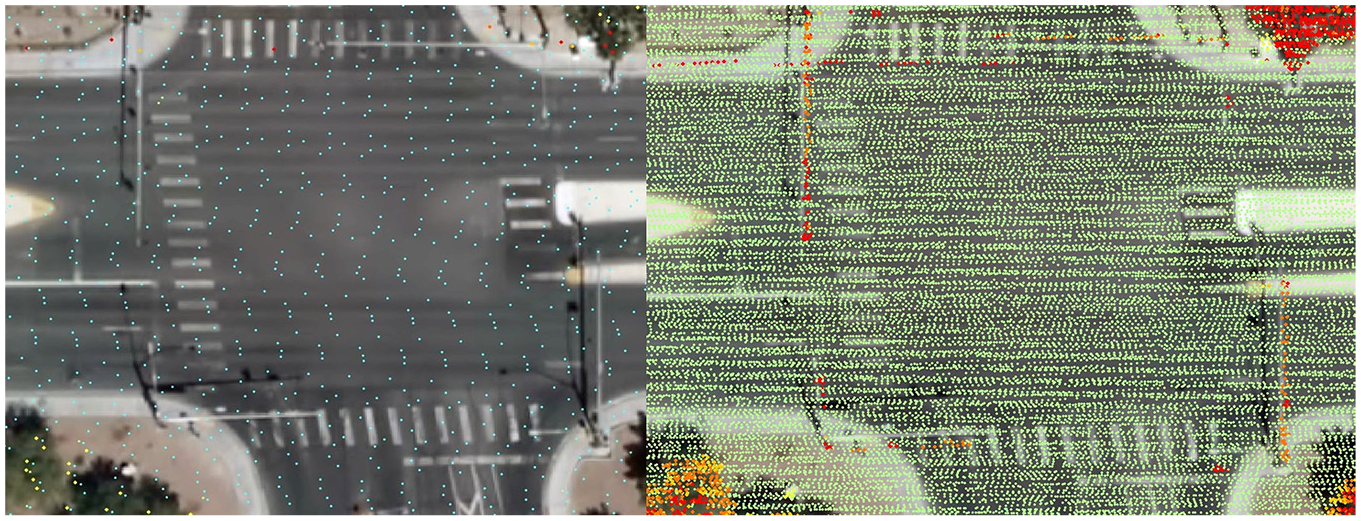
Example of LiDAR QL2 and QL1 data for the same intersection: QL2 (left), QL1 (right).

Golombek and Marshall ( 5 ) explored the limits of QL2 data by designating streetscapes in three-dimensional (3D) pixels—better known as “voxel” grids—and found that QL2 data for measuring streetscapes is primarily limited to buildings and street trees. Since understanding the impacts of street trees and other clear zone objects is an important transportation topic, that study also discussed how 3D measurement of street trees widely differs from traditional 2D-derived canopy data. Specifically, the vertical components of the street trees were defined by the vertical voxel zone or voxel interval they fell into. Though QL2 is currently the more common USGS specification, LiDAR technology is evolving rapidly, more specifically, from a point density of one point per five square meters in the mid 1990s to QL1 standards being the norm in the near future ( 6 ). With public QL1 data becoming more common and being four times denser than QL2, QL1 is expected to be able to measure discrete streetscape features objectively well beyond QL2’s buildings and trees.

In relation to transportation research, finding objective methods to measure streetscapes and streetscape features is important for measuring perceptual qualities of streetscapes as well as for transportation-related outcomes such as those related to road safety. Perceptual qualities, such as “street enclosure,” among many others, have long been studied and analyzed by urban planners and designers trying to understand the qualities and characteristics of streetscapes that make them more appealing and desirable. Published work on perceptual qualities began in the late nineteenth century with Camillo Sitte ( 7 ) and continued through the twentieth, as Gordon Cullen ( 8 ), Donald Appleyard ( 9 ), Anotol Rapoport ( 10 ), and Henry Arnold ( 11 ) all produced literature addressing the importance of perceptual qualities in urban design. More recently, since around 2010, research has focused more on improving measuring techniques. The next section discusses how buildings and street trees have been measured in recent streetscape studies. Smaller and essential streetscape features–such as streetlights, signs, landscape features, and streetscape furniture–have not yet been incorporated in such studies.

In relation to road safety outcomes, conflicting research exists around the role of streetscape features. For instance with street trees, the research findings have long been contradictory over their influence on road safety outcomes ( 12 – 14 ). Some studies suggest that street trees are associated with better safety outcomes ( 15 ), while other studies find them to be hazardous ( 13 , 16 ). Aside from street trees, transportation research has also focused on how physical characteristics of other streetscape features enhance safety. Placement and characteristics of streetlights have an effect on pedestrians’ perceived safety ( 17 ). The same is true in relation to measurements, placement, and dimensions of streetlights ( 18 , 19 ) as well as street sign placement for drivers ( 20 , 21 ). Along with these features, utility poles and other fixed objects in streetscapes have been shown to affect transportation outcomes ( 14 ).

With QL1 data becoming more publicly available, the goal of this study is to determine what role LiDAR data collected at QL1 standards can play in transportation research. Specifically, this study attempts to extract and measure quantitatively the common streetscape features mentioned above, in addition to street trees and buildings common to QL2 data analysis. This study will present a comprehensive methodology for measuring 3D characteristics of streetscape features—based on voxel (3D pixel) zones—using USGS QL1 data for the purpose of compiling objective descriptive statistics of how these features are represented in 3D streetscapes. To compile the descriptive statistics from the voxels, where features fall will be processed into compiled voxel height intervals, like the data shown in Figure 2. The voxel-feature data will ultimately be converted into vector data to compile tabular descriptive statistics. If the assessment can be adequately performed with QL1 data, then it can become common practice and more widely applied in municipalities (where QL1 data already exists) and eventually in municipalities across the U.S. for assisting the assessment of 3D characteristics of features within streetscapes.

Figure 2.

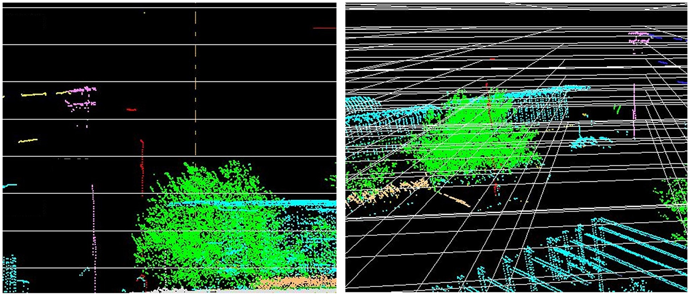
Example of voxel grid over streetscape features (left image represents a vertical view; right image represents a diagonal view).

Literature Review

Over the past two decades, improving remote sensing technologies and emerging geographic information systems (GIS) applications have affected transportation research in ways such as how streetscapes are measured and understood in relation to outcomes such as livability, physical activity, and road safety. Over that time, streetscape measuring methods have evolved to become more objective.

Before implementing streetscape measuring with mapping technologies, methods were more audit based. Ewing et al. were among the first urban design researchers to implement audit-based measurement techniques within streetscapes ( 22 – 24 ). These authors developed and implemented a comprehensive manual to guide field observation for quantitative measures to pair with concepts such as streetscape desirability and walkability. Brownson also compared a significant number of audit-based techniques ( 25 ) to measure the built environment as it relates to physical activity. Brownson acknowledged that these measures are time consuming. His study listed dozens of observation-based instruments that can take up to 20 min per street segment to calculate for each method. According to Brownson, the auditors were often students who often did not have a technical skillset for auditing. Yin mentioned that individuals conducting estimated measures through audits often perform subjective observations, which can be inconsistent across observers ( 26 ).

Auditing seems to have subsided, at least to some extent, as GIS and its spatial data analytics became more mainstream. Purciel et al. attempted to implement GIS measures to offset complexities involved with manual audit-based assessments of streetscape and assessed their results against Ewing et al.’s outcomes. They used New York City to measure streetscape features and variables for five primary perceptual qualities of streetscapes: imageability, enclosure, human scale, transparency, and complexity. The data that Purciel et al. used was simple 2D GIS polygon data features resulting from various public sources and tabular data. Results acknowledged correlations between GIS and observed measures that ranged from 0.28 to 0.89 ( 27 ). This wide and varying correlation range is hard to comprehend because the GIS data and the observed measures the GIS data was weighted against contain a lot of subjectivity in the data and methods.

A study by Yin and Shiode went beyond simple GIS data and appended 3D attributes to 2D GIS features to evaluate streetscape measures related to walkability research conducted by Ewing and Handy ( 23 ) and Purciel et al. ( 27 ). In Yin and Shiode’s study, GIS and remotely-sensed aerial photographs were utilized to extract buildings and trees, among other features. Height attributes from the assessor database gave buildings their heights, and trees were grouped into small, medium, and large categories. Yin’s study built on these previous works by using remotely sensed imagery and 3D GIS to measure street-level urban design qualities objectively and test their correlation with observed data. The statistical results concluded that 3D GIS helped generate objective measures on view-related variables. Yin’s data was more objective than simple 2D GIS data; yet, it was still subjective since the 3D components were simply derived from measurement extrapolations appended to 2D GIS data of features such as trees and buildings. These 3D GIS methods did, however, yield some improvements to correlations with walkability scores established by Ewing and Purciel ( 26 , 28 ).

Harvey et al. took their objective 3D streetscape mapping techniques even further than Yin and Shiode. Harvey et al. published two research articles ( 29 , 30 ) utilizing advanced GIS methods and high precision data (including LiDAR) to measure streetscape skeletons. In both articles, the primary focus was on the buildings surrounding the streetscapes discussed as part of the street’s enclosure matrix, and the authors discussed the perceived safety of these environments. Though street trees are touched on, the authors noted that walls, fences, streetlights, and other design elements were unaccounted for because of the lack of adequate spatial data. Also, the authors noted that these features may be insignificant because they “embellish the broader streetscape already defined by buildings that dwarf them in size,” alluding to their relative insignificance because of surrounding buildings (30). It is important to note that these studies take place in high-density areas, primarily New York City, but also Boston and Baltimore, where streetscapes are more enclosed by buildings on each side than in most other cities. The majority of urban streetscapes in the U.S. do not have significant buildings to fill the enclosure matrix. Therefore, the common streetscape features that are unaccounted for may be critical for mapping typical urban streetscapes in the U.S. since they are features of streetscape focus in the absence of buildings encroaching on roadways.

Harvey and Aultman-Hall also conducted a comprehensive study in New York City in 2015 incorporating nearly 240,000 crashes for over 75,000 road segments ( 31 ). This study incorporated many variables, including LiDAR-derived 2D tree polygons, GIS building data, and cross-section width between buildings to weigh street enclosure perceptions to crash outcomes. However, this study appears to analyze 2D tree polygon coverage area only within a streetscape, neglecting LiDAR’s capabilities to assess 3D tree features. For example, if two streetscapes had 15% total tree coverage, one could have significantly more tree density/biomass because the 3D characteristics are not considered. It is such characteristics that may be critical for understanding the impact of urban streetscape features on transportation-related outcomes.

The authors’ recent streetscape LiDAR study ( 5 ) discussed streetscape features that can be extracted from USGS QL2 data. That study determined that QL2 data is limited to extracting buildings and trees in the streetscape. Since other studies linking LiDAR building classifications with building footprints show strong correlations ( 32 , 33 ), and since street trees are a significantly analyzed topic in transportation research, the study examined and found significant statistical differences between deriving 3D characteristics of trees against 2D LiDAR-derived polygons. QL2 data is limited in relation to usefulness for transportation-based feature extraction, however, as many more critical features other than building and trees exist in a typical streetscape environment.

Research extracting streetscape features (aside from buildings and trees) from LiDAR is limited. Recently, a cut-graph segmentation method was used with mobile LiDAR to extract urban street poles automatically, resulting in a 90% success rate ( 34 ). Unfortunately, QL1 data is not nearly dense enough to apply this method, and the methods section below explains why automated processes in general are not applied to this research. Mobile LiDAR is far denser than QL2 or QL1 LiDAR, but mobile LiDAR typically requires private collection, and processing is slow and labor intensive because of its high point density. This research study attempts to analyze publicly available USGS QL1 LiDAR data to extract and measure a variety of smaller and more discreet streetscape features that could not legitimately be detected in a common QL2 dataset.

Data and Methods

Overview

Aside from street trees and buildings derived from QL2 LiDAR data ( 5 ), other features common to typical urban streetscapes include light poles/lampposts, power lines, landscape features, traffic signals, street signs, property walls/fences, and street furniture. Research on roadside landscape improvements has been linked to safer driving environments ( 35 – 37 ). Quantities and positions of street lighting can also affect safety within streetscapes ( 17 , 38 ). Response time to street signs affects transportation outcomes ( 21 ), and measurement and location of street signs are likely correlated with response time. Roadside walls and street furniture affect various perceptual qualities when assessing streetscapes for walkability and desirability ( 22 , 24 ).

Harvey et al. ( 29 , 30 ) are among the few researchers to have utilized advanced geospatial data and methods to measure streetscape features. They acknowledge, however, that publicly available remote sensing data is not advanced enough to detect these common streetscape features. Therefore, the methods presented in this study will analyze and identify approaches to mapping and measuring these distinct features that were previously cited as undetectable. In doing so, it will assess how each individual street corridor/streetscape section is statistically composed of the streetscape features the authors are trying to extract from QL1 data. Sectionalized voxel zones at specified intervals are used to understand how common streetscape features noted above can be quantified and measured in 3D. This study will show a descriptive statistics output model of this data that can be applied to transportation research studies. In geospatial terms, a voxel is a 3D pixel and will be discussed in depth later in this section. To conduct this study, an urban QL1 dataset is required.

Data

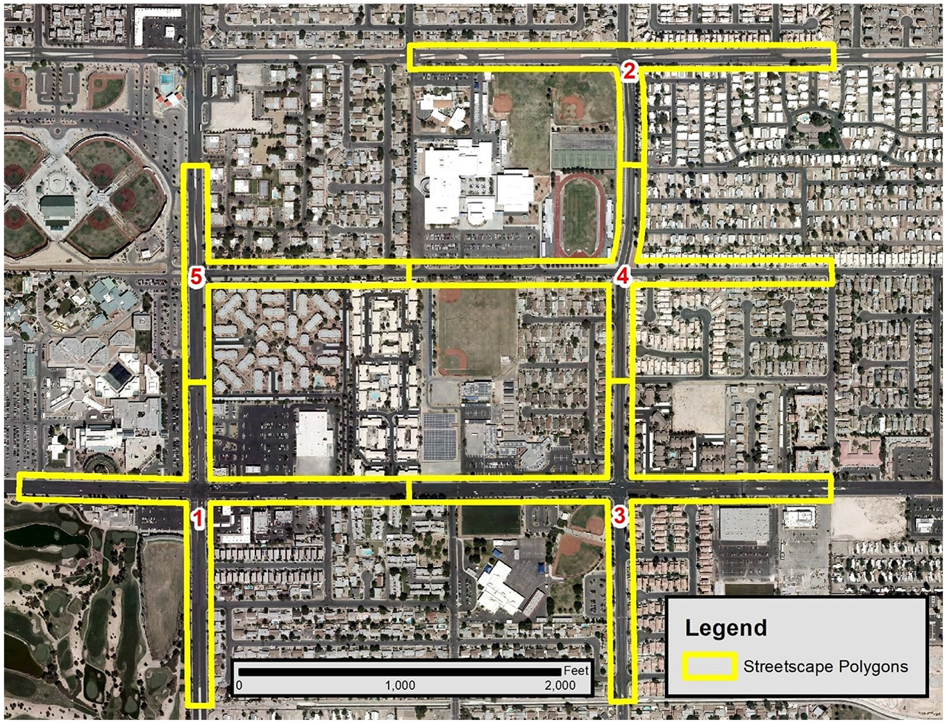
QL1 data of Las Vegas is currently publicly available via the USGS National Map website. This environment was chosen since streetscape features in urban Las Vegas, with its desert environment, appear distinct and separate from one another and will therefore provide a good baseline in relation to our ability to detect them within QL1 point cloud data. The large size of these datasets covering the area of interest (AOI), however, make them prone to data noise. Fortunately, USGS requires its LiDAR collection vendors to place all noise data on a separate point cloud classification layer ( 39 ). USGS then runs internal proprietary checks to assure noise mitigation compliance. Therefore, additional noise mitigation is not necessary. The AOI is a sample section in urban Las Vegas amounting to 12 street segments, encompassing around four linear miles of streetscape, and specifically, five streetscape sample areas polygons. Six-inch aerial imagery, simultaneously collected with the LiDAR data that covers the AOI, was also used for referencing when needed.

Methods

Creating Streetscape Sample Areas

Since the aim is to append quantitative statistics of streetscape features within a streetscape, it is important to devise an adequate method to create individual streetscapes. Creating individual streetscape corridors means that a segment will have a cutoff, either in its center or through the intersection. A preliminary look at our sample area shows that long overhanging traffic signals and light posts may be cut off if the streetscape is divided at the intersection. Also, intersections tend to be focal areas with high activity and thus more traffic-related features. Therefore, a method to cut off the segments between the intersections rather than the middle of them is preferred for this study.

The AOI is divided into Thiessen proximal polygons (or Voronoi polygons, as mathematicians call them). The ESRI ArcGIS^® Thiessen polygon processing tool is used and the street intersection centroids input for the polygon center-points. Thiessen polygon datasets are mutually exclusive and non-overlapping. Thiessen polygons are used in this model because they divide the polygons (streetscapes, in this case) in a clean and somewhat uniform manner and can be created with a GIS application around a designated focal point set. The intersection centers were used as centroids for this focal point set. The Thiessen/Voronoi method gives weights to high event/focal areas and is a popular model and spatial method for focusing on focal event points ( 40 ).

Additionally, the streetscape sample areas are designed to include the full street right-of-ways that extend 10 ft to 20 ft beyond the street curb. Extending the streetscape to include these peripheral views within the streetscape is important since the majority of objects that constitute a streetscape’s perceptual qualities are located off the street itself ( 24 ). Furthermore, the parcel data for the AOI is joined and used to erase all non-streetscape right-of-way areas, resulting in the sample areas in Figure 3.

Figure 3.

Area of interest and streetscape polygons; red numbered streetscape polygon IDs link to Tables 1 and 2.

Table 1.

Descriptive Statistics of Streetscape Features from the QL1 Sample Dataset Derived from Voxel Intervals

Streetscape polygon	Percent tree coverage	Tree density^a	Landscape area (sq. feet)	Building area (sq. feet)	Percent building coverage	Overhanging street light count^b	Overhanging street light area (sq. feet)^b	Light Pole only count^c	Light pole only area (sq. feet)^c	Sign count	Wall length (feet)	Traff light area (sq. feet)	Electic pole count	Electric line^d length (feet)	Street furniture count	Street furniture area (sq. feet)
Zone 1 (0–5 ft)
1	0.05	1.13	24453	5813	0.90	0	0	76	955	22	2056	0	5	0	17	2759
2	0.17	1.32	7776	10616	2.18	0	0	48	603	21	3943	0	12	0	10	743
3	0.14	1.11	13950	37279	5.56	0	0	68	2321	43	3815	0	0	0	14	1056
4	0.13	1.03	5202	78946	13.73	0	0	31	390	27	2466	0	0	0	14	1479
5	0.16	1.09	9693	47809	12.27	0	0	31	389	11	1955	0	0	0	5	347
Zone 2 (5–10 ft)
1	2.95	1.43	5733	5813	0.90	0	0	76	955	22	2025	0	5	0	10	1413
2	4.13	1.15	756	10616	2.18	0	0	48	603	21	3557	0	12	0	5	430
3	3.44	1.06	1233	37279	5.56	0	0	68	2321	43	3750	0	0	0	8	784
4	3.54	1.18	1368	78946	13.73	0	0	31	390	27	2431	0	0	0	5	942
5	4.00	1.31	6381	47809	12.27	0	0	31	389	11	1955	0	0	0	4	316
Zone 3 (10–15 ft)
1	4.26	1.53	0	4873	0.76	0	0	76	955	0	0	0	5	0	4	529
2	6.08	1.08	0	8597	1.77	0	0	48	603	0	0	0	12	0	2	245
3	5.36	1.19	0	36380	5.42	0	0	68	2321	0	90	0	0	0	1	118
4	4.70	1.25	0	78796	13.70	0	0	31	390	0	0	0	0	0	1	115
5	6.61	1.62	0	35687	9.16	0	0	31	389	0	0	0	0	0	1	11
Zone 4 (15–20 ft)
1	3.60	1.45	0	4218	0.66	0	0	76	955	0	0	163	5	0	0	0
2	4.40	1.08	0	2306	0.47	0	0	48	603	0	0	0	12	0	2	245
3	5.08	1.17	0	31143	4.64	0	0	68	2321	0	90	0	0	0	1	118
4	4.15	1.25	0	43481	7.56	0	0	31	390	0	0	0	0	0	1	115
5	4.80	1.61	0	22024	5.65	0	0	31	389	0	0	0	0	0	0	0
Zone 5 (20–25 ft)
1	2.94	1.38	0	3501	0.54	0	0	76	955	0	0	468	5	0	0	0
2	2.78	1.11	0	246	0.05	0	0	48	603	0	0	735	12	0	0	0
3	3.80	1.20	0	22312	3.33	0	0	68	2321	0	90	901	0	0	1	118
4	3.06	1.18	0	8905	1.55	0	0	31	390	0	0	0	0	0	0	0
5	2.78	1.74	0	9829	2.52	0	0	31	390	0	0	657	0	0	0	0
Zone 6 (25–30 ft)
1	1.87	1.52	0	1750	0.27	1	31	76	955	0	0	0	5	1287	0	0
2	1.82	1.04	0	123	0.03	3	93	48	603	0	0	0	12	2641	0	0
3	3.10	1.37	0	11156	1.66	2	62	68	2321	0	90	0	0	0	0	0
4	2.42	1.11	0	4453	0.77	0	0	31	390	0	0	0	0	0	0	0
5	1.68	1.39	0	4915	1.26	0	0	31	390	0	0	0	0	0	0	0
Zone 7 (30–35 ft)
1	1.25	1.49	0	0	0.00	61	1891	74	930	0	0	0	4	0	0	0
2	1.02	1.10	0	0	0.00	43	1333	45	566	0	0	0	12	0	0	0
3	2.48	1.30	0	0	0.00	54	1674	64	1110	0	90	0	0	0	0	0
4	2.02	1.01	0	0	0.00	31	961	31	390	0	0	0	0	0	0	0
5	1.24	1.41	0	0	0.00	25	775	31	380	0	0	0	0	0	0	0
Zone 8 (35–40 ft)
1	0.72	1.48	0	0	0.00	6	186	4	50	0	0	0	4	640	0	0
2	0.45	1.24	0	0	0.00	7	221	2	25	0	0	0	12	0	0	0
3	1.87	1.32	0	0	0.00	5	155	8	407	0	0	0	0	0	0	0
4	1.12	1.23	0	0	0.00	0	0	0	0	0	0	0	0	0	0	0
5	1.12	1.25	0	0	0.00	5	155	4	50	0	0	0	0	0	0	0
Zone 9 (40–45 ft)
1	0.42	1.47	0	0	0.00	0	0	0	0	0	0	0	1	0	0	0
2	0.23	1.45	0	0	0.00	0	0	0	0	0	0	0	12	0	0	0
3	1.03	1.35	0	0	0.00	0	0	8	407	0	0	0	0	0	0	0
4	0.34	1.01	0	0	0.00	0	0	0	0	0	0	0	0	0	0	0
5	0.78	1.43	0	0	0.00	0	0	0	0	0	0	0	0	0	0	0
Zone 10 (45–50 ft)
1	0.10	1.15	0	0	0.00	0	0	0	0	0	0	0	0	0	0	0
2	0.15	1.13	0	0	0.00	0	0	0	0	0	0	0	8	2641	0	0
3	0.37	1.75	0	0	0.00	0	0	6	345	0	0	0	0	0	0	0
4	0.01	1.14	0	0	0.00	0	0	0	0	0	0	0	0	0	0	0
5	0.18	1.88	0	0	0.00	0	0	0	0	0	0	0	0	0	0	0
Zone 11 (50–55 ft)
1	0.00	1.00	0	0	0.00	0	0	0	0	0	0	0	0	0	0	0
2	0.04	1.39	0	0	0.00	0	0	0	0	0	0	0	0	0	0	0
3	0.03	2.00	0	0	0.00	0	0	5	314	0	0	0	0	0	0	0
4	0.00	0.00	0	0	0.00	0	0	0	0	0	0	0	0	0	0	0
5	0.03	0.71	0	0	0.00	0	0	0	0	0	0	0	0	0	0	0
Zone 12 (55–60 ft)
1	0.00	0.00	0	0	0.00	0	0	0	0	0	0	0	0	0	0	0
2	0.02	1.58	0	0	0.00	0	0	0	0	0	0	0	0	0	0	0
3	0.00	0.00	0	0	0.00	0	0	5	314	0	0	0	0	0	0	0
4	0.00	0.00	0	0	0.00	0	0	0	0	0	0	0	0	0	0	0
5	0.04	1.16	0	0	0.00	0	0	0	0	0	0	0	0	0	0	0

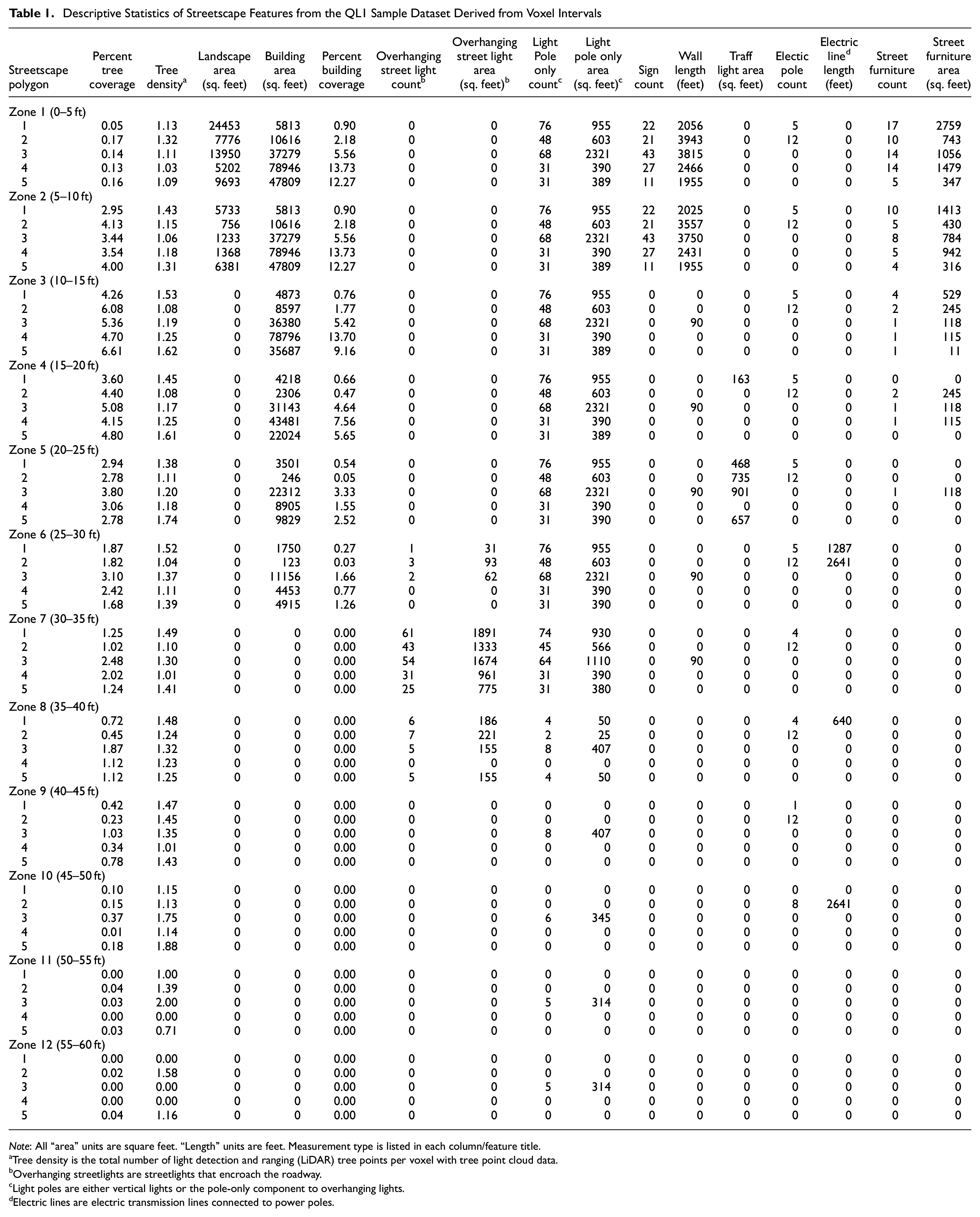
Note: All “area” units are square feet. “Length” units are feet. Measurement type is listed in each column/feature title.

Tree density is the total number of light detection and ranging (LiDAR) tree points per voxel with tree point cloud data.

Overhanging streetlights are streetlights that encroach the roadway.

Light poles are either vertical lights or the pole-only component to overhanging lights.

Electric lines are electric transmission lines connected to power poles.

Table 2.

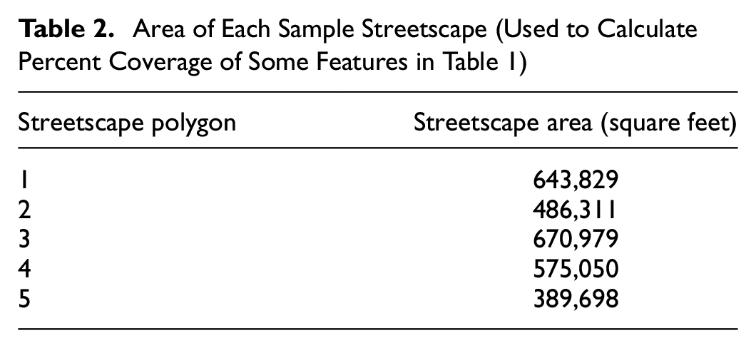
Area of Each Sample Streetscape (Used to Calculate Percent Coverage of Some Features in Table 1)

Streetscape polygon	Streetscape area (square feet)
1	643,829
2	486,311
3	670,979
4	575,050
5	389,698

Devising 3D Streetscape Extents

As mentioned, this study incorporates 3D pixels, or voxels, to quantify streetscape features. A significant component of this proposed method is voxelization of the street segments to quantify street features and understand how the features are represented in 3D space, specifically different height zones within a streetscape. As mentioned, QL1 LiDAR emits around eight survey points per square meter, so it is expected that above-ground streetscape features will absorb these points to a much higher degree than the far less dense QL2 data. This study will provide area and length statistics of discernable streetscape features within the voxel height zone in which it appears. The features will be grouped by each streetscape section/feature.

A voxel is a pixel with a height or third dimension component when analyzed with LiDAR. Figure 2 shows an example of LiDAR enclosed in voxels. Optimizing the vertical and horizontal height of the voxel depends on the features detected and the spacing of LiDAR data. USGS standards stress the importance of consistency of point patterns for horizontal spacing throughout a dataset and sets a standard for spatial distribution of at least one point per grid cell ( 39 ). However, with QL1 data having a nominal point spacing greater than one point per every half-square-foot, adhering to these minimum standards is not necessary because tiny grid cells would cause datasets to be large in size and difficult to process.

When setting the vertical voxel dimensions, it is important to consider occluded LiDAR data. Dense tree canopies can occlude LiDAR data. Voxels that were completely hidden from the laser instrument are considered occluded. Occluded voxels are voxels that are theoretically traversed by the pulses, meaning the pulses would have reached the voxel, but all energy was already intercepted because of earlier interactions of the laser pulses with canopy material ( 41 ). An in-depth study by Kukenbrink et al. is one of the few studies that address occluded voxels and attempt to minimize their presence. In a recent study investigating streetscape measuring with QL2 data ( 5 ), the authors investigated Kukenbrink et al.’s results and conclude that a voxel height of 5 ft is ideal for both limiting occluded data and providing adequate vertical intervals or zones for analysis.

As QL1 data has a nominal point spacing of around 0.4 ft, and per the USGS standard for horizontal grid spacing, the horizontal cell size can be set much smaller than the 5 ft vertical spacing. However, setting the horizontal parameters too small would skew the voxel significantly. Since optimal street tree collection limits the setting of the voxel to 5 ft, this study will use the horizontal dimensions of 3 ft by 3 ft used previously in the authors’ successful QL2 study. Therefore, the streetscape will be set up into 5 ft elevation zones with each classified pixel having 3 ft by 3 ft dimensions.

Classifying Streetscape Data

LiDAR data classification is either performed manually or by automated filtering processes. Creating bare-earth models is the most common automated process, though automated processing to filter LiDAR data specifically for trees and buildings is also common. Road and grassed areas are other features that have automated extraction capabilities from aerial LiDAR ( 42 ), though this study is not concerned with features on the ground. A 2012 study by Shyue et al. attempted to incorporate hybrid approaches to assist with urban feature extraction, yet that study was limited only to buildings, trees, grass, and roads ( 43 ). Methods are emerging to extract street poles from LiDAR automatically ( 34 ), though the methods specified for doing so from street-based mobile LiDAR as opposed to the open source and publicly-available USGS data. Since automated methods for extracting streetscape features with QL1 data are not publicly available, the authors defer to manual classification of features common to LiDAR feature extraction in general. As mentioned above, buildings and trees are classified via automated processes.

When LiDAR hits non-solid vegetation, the energy of the light pulse continues to the ground and records each instance, or return, of vegetation hits until it reaches the ground. The exception to this is when tall and thick vegetation occlude the LiDAR. In general, LiDAR will stop at the first solid feature it hits. Therefore, three types of above-ground objects LiDAR can hit are:

A hanging object in space: examples include the arms of light poles and power lines.

A continuous object: specifically, an object that continues all the way to the ground. Examples include a property wall, building, power pole, and base of a light pole (Figure 4).

Vegetation: a multi-point return object such as a tree.

Figure 4.

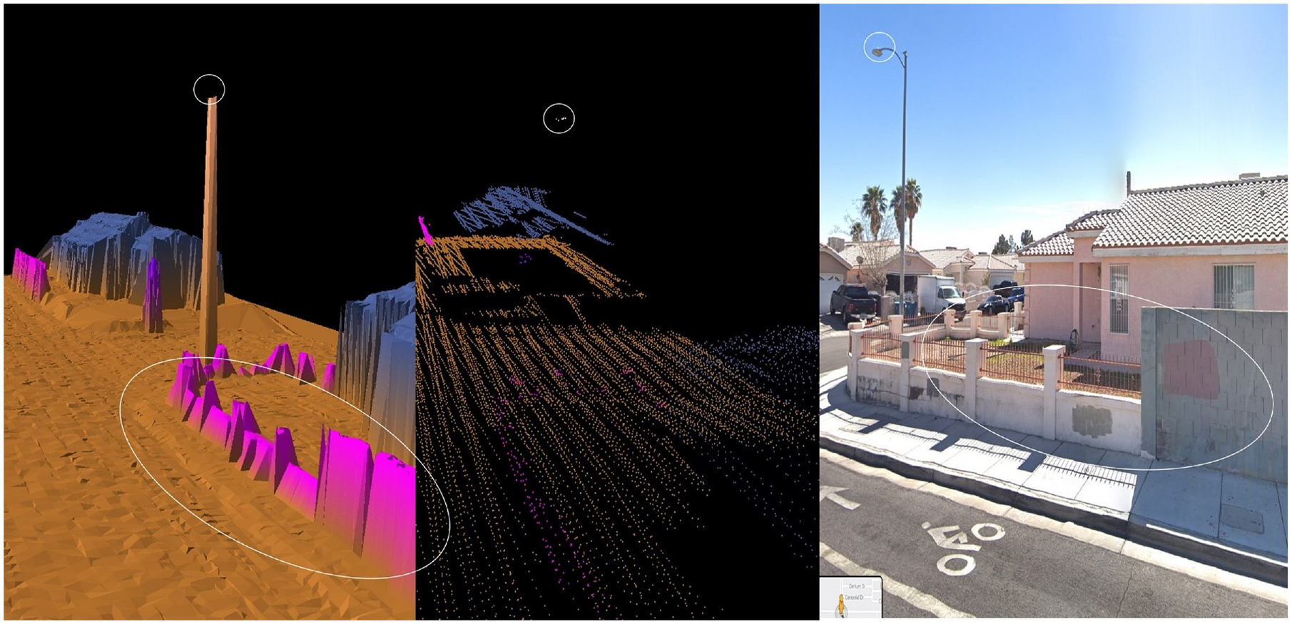
Example of draped features. Light pole base, house, and fence are draped to ground (left); fence features appear like actual fence from Google StreetView (right).

Type 1 above will be represented by where the point hits the voxel that contains the feature. Type 2 will also be represented by where the point hits the feature/voxel; however, the features will be captured and noted with a 3D shapefile so that the entire feature is draped to the ground through its lower voxel zones. Type 3 will utilize automated, multi-point return vegetation extraction processes common to LiDAR processing software. Vegetation multi-point returns are clusters of LiDAR points that intercept multiple targets within a short height interval. In this case, trees that are common to Las Vegas will be noted. Palm trees, for instance, tend to have small elevated canopies with long trunks, as opposed to most deciduous trees. If necessary, the 3D draping of features will be utilized like the continuous objects (type 2), so the long standalone trunks are represented as well.

An automated LiDAR feature extraction method is preferred when extracting various feature classes covering a large area. After an extensive literature review, it appears that automated methods have not materialized to classify most streetscape features beyond street trees and buildings derived from aerially-collected QL1 data. This study used common automated LiDAR processing tools available within MARS^® software to classify buildings and trees. The above literature review cites research that automatically classifies streetlights ( 34 ), though the dataset used was mobile LiDAR, which is dozens of times denser than publicly available QL1 data. Reviewing recent research attempting to extract urban features automatically ( 44 , 45 ), researchers utilize manual classification of point cloud data for truthing their automated methods, likely because of LiDAR’s highly accurate positional characteristics. These studies utilize LiDAR data densities like QL1 but do not extract any additional necessary streetscape features discussed except powerlines. The isolated nature of powerlines makes them easily detected when already classifying features manually. Since previous research focused on a manual method for automated process truthing, along with LiDAR’s highly accurate output, this study utilizes similar manual classification to accurately compile the streetscape feature classes. In the case of the manually classified USGS QL1 point cloud, the data will have relative accuracy or root mean square error of within 1/3 ft vertical and within 1 ft horizontal based on USGS specs and collection metadata ( 39 , 46 ).

Merrick and Company’s MARS^® LiDAR processing software was utilized to classify the LiDAR data manually. MARS^® has a feature to pair Google Earth with any current LiDAR view. Per Figure 5, this pairing allows for the LiDAR data to be present on one computer screen and Google StreetView’s identical location to be present on an adjoining computer screen. With highly accurate USGS LiDAR data, the MARS^®/Google dual visual setup/pairing allows for accurate and seamless classification of the various feature classes noted below.

Figure 5.

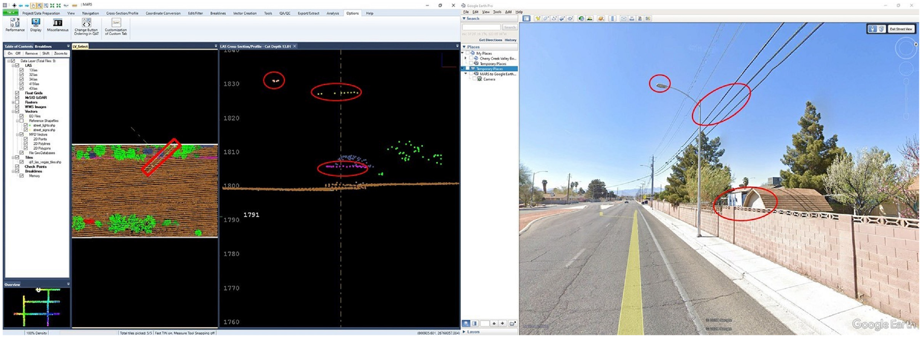
Example of Google view paired with MARS^®. Rectangular box at far-left view shows profile box. Left-center view shows light detection and ranging (LiDAR) data visible in profile view. This is where manual classification occurs. Right view is paired Google view to assist with seamless manual classification.

MARS^® was also used to establish and process data into the voxel zones. The features described below can be processed into the noted voxel zones. Aerial LiDAR scan angles can cause parts of small features to be missed. For example, thin overhead electric lines and arms of overhanging light posts may be captured at nadir but missed when the scan angle is too high. Therefore, ESRI ArcGIS^® are used to draw polygons around feature point cloud clusters with high resolution imagery to help complete line and polygon features when necessary. A tool in MARS^® will populate constructed polygons with applicable z-values. A LiDAR generated ground elevation grid is then used to subtract feature height from ground, to determine the exact height above ground of classified and processed features, and to be sure they are classified into the correct voxel zone. Since the City of Las Vegas collects and maintains Global Positioning System (GPS) data for all its streetlights and street signs, the municipal GPS point data was also used as an additional check to confirm the streetlights and street sign base locations. The counts in this study matched the City’s counts.

Figure 6 below shows the difference between a QL1 and QL2 dataset for the same intersection in relation to these streetscape features. Unlike QL2 data, it is assumed that many features stand out with QL1 data and can be properly classified. The authors’ QL2 study ( 5 ) already discussed extracting the following features:

Tall trees (any vegetation with a trunk, not classified as landscape vegetation): Common automated processes classify street trees. The points in the first zone were manually classified when classifying landscape vegetation. The automated process was set to exclude the lowest zone because of interference of urban reflecting objects ( 47 , 48 ).

Buildings: Buildings and houses enter the streetscape peripherally. Common LiDAR processing procedures were used to create building polygons and a height attribute helped place these features into voxel zones. Since the height is always the top voxel zone, the building is then draped through the lower voxel zones until it reaches the ground.

With high-density QL1 data, the authors attempted to explore the limits of this LiDAR data standard and to extract all additional above-ground features that make up a streetscape. These features include the following:

Walls/fences: LiDAR points on top of walls and fences are clearly discernable. Lines are drawn across these points and are draped to ground level.

Landscape vegetation (low brush): Though LiDAR acceptably detects vegetation through an automated process, low-lying vegetation is best classified manually as obstructions causing interference can distort data. In the present example, landscape features are easily discerned when LiDAR is overlaid with either imagery collected simultaneously with the LiDAR or pairing LiDAR street-scenes with Google StreetView, as mentioned above.

Tall trees (low zone[s] only) as noted in the QL2 description above, the lowest zones are manually classified,

Light posts: These generally have two parts. Light post LiDAR points are clearly seen, and elevation is extracted. If the light is overhanging a street, a polygon is constructed around the clustered points and that polygon is inserted into the appropriate voxel zone. The second part is the vertical post (or non-overhanging streetlight), which is split off from an overhanging light and draped through the voxel zones to the ground.

Traffic lights: In this sample set, traffic light points are easily discerned. A polygon is drawn around the clustered points and placed into its respective voxel zone.

Power poles/lines: The poles are clearly distinguished. The lines are hit and miss. The poles are captured and draped. Since we know lines generally connect to poles in streetscapes, the available line points are connected, and Google StreetView is used to verify.

Street signs: Street signs are often connected to light posts and power poles. When they are independent, they generally have a few LiDAR points. In our sample set, all signs are within the first two voxel zones, as noted in the results below.

Additional street furniture (anything on the sidewalk or median not noted above, such as benches, bus stops, garbage cans, etc.): QL1 data successfully captures many street furniture features such as pedestals, bus stops, large garbage cans, multiple residential mailboxes, large benches, and non-traffic signs, to name a few. Unfortunately, some are too small to distinguish such as common fire hydrants and small benches. Most street furniture features are within the first voxel zone.

Figure 6.

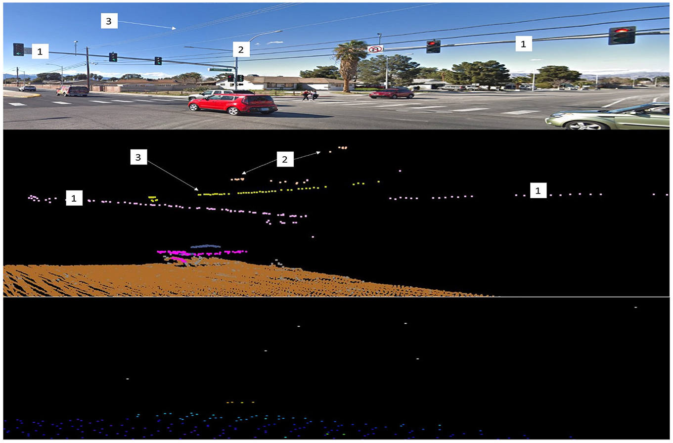
Sample views of an intersection: (top) Google StreetView; (middle) QL1 image: 1 = traffic lights, 2 = dual streetlight, and 3 = power lines; (bottom) same view with lower quality QL2 data.

The voxel processing tool generates an individual height-zone raster grid for each streetscape feature that was classified. The raster grids are converted into vector features ultimately to calculate percentage coverage, counts, or feature length, as noted in Table 1. When processing is complete, descriptive statistics in tabular format of the noted features above are represented in each streetscape segment, also noted in Table 1.

Results and Discussion

The results of this study enable access to an array of objective descriptive data not previously available, as USGS QL1 publicly available data is relatively new. When downloading, processing, and classifying streetscape QL1 data via these methods, researchers can obtain quantifiable 3D characteristics of streetscapes to apply to various transportation research needs. Table 1 shows sample descriptive statistics available and how they are broken into their relevant height zones. Table 2 shows the areas for each corresponding polygon in Figure 3 above.

Note that Table 1 is an extensive example. For instance, the percentage of tree coverage as a whole for each streetscape polygon is noted in the first column of Table 1. The results show tree coverage initially increases and then decreases toward the higher zones. For example, the highest tree coverage recorded for any sample area in any zone is 6.61% coverage in zone 3, which is the 10–15 ft zone. Buildings show similar results. Table 1 has both linear coverage and total percent coverage for buildings. Since typical buildings or dwellings are widest at ground level, statistics show how building coverage is highest at the low height intervals and reduces in coverage as the intervals increase. For example, sample area #4 in Table 1 shows 13.7% coverage in the initial two zones, yet by zone 6 (between 20 ft and 25 ft above ground) coverage for this sample area is below 2%.

It is important to display an extensive example of the descriptive statistics available, since many streetscape features are detectable with QL1 data, and researchers may have an interest in quantifying different features for different reasons. These statistics can be quantified by counts, lengths, and areas. Area relates to voxel horizontal area coverage per zone. For linear features like walls/fences and power lines, feature length is detected by digitizing the classified features with a best-fit 3D polyline. For example, take 150 ft of continuous point cloud classified as wall 10 ft above ground. Given the 5 ft vertical setting for each voxel, and the continuous object draping method mentioned previously, that wall would contribute 150 linear feet in zone 1 and 150 linear feet in zone 2. For the sample areas, wall lengths were detected that varied from 1,955 square feet to 3,943 square feet. After zone 2, the voxel zones show “0” for wall length because the dataset does not have any walls of fences above 10 ft, except sample area 3 that had 90 ft of tall fence surrounding a sports field.

As mentioned in the introduction, there are conflicting research findings about the impact street trees and landscape improvements have on road safety, and one possible source of conflict has been our inability to measure these features properly. The authors’ previous study exploring the limits of USGS QL2 data expresses and legitimizes voxel use for measuring trees ( 5 ). Though some manual classification is involved with the QL1 process, actual objective and measurable landscape features can coincide with street tree data to assist with such research.

Evaluating buildings and how they encroach streetscapes has been done in the past. However, studies can now incorporate objective data that takes into account building characteristics based on highly-accurate measured outcomes as opposed to crude building outlines commonly available with open source GIS data. Furthermore, street walls/fences are objectively measured in both length and height. Though this study is limited in that not every piece of street furniture can be legitimately extracted, many are. Ewing and Clemente ( 24 ) discuss in their research the importance of these types of features for measuring perceptual qualities of streetscapes such as enclosure, human scale, and transparency, which can now be objectively measured and compared with previous crude methods.

When looking at Table 1, it is interesting to note the diversity of height-space. Some features such as street trees are covered throughout. Others such as street furniture, street signs, and landscape features are in the lower zones. Traffic lights and overhanging streetlights do not hit a low voxel zone. Similar to previous streetscape research relying on 2D-derived polygons, these types of features have yet to be applied to transportation research incorporating their 3D measurements. The diversity of space shows how quantitative 3D groupings of data is much different than crude 2D data, and thus, can lead to different results when applied to transportation research outcomes.

The literature review noted the recent streetscape measuring studies done by Harvey et al. that have produced some extensive and comprehensive work on the topic. Harvey et al. specifically mentioned in two of their studies that smaller features such as walls, fences, streetlights, and other design elements are typically unaccounted for because of lack of adequate spatial data ( 29 , 30 ). The above results completely change that assumption, and as QL1 data becomes more mainstream, so will the ability to incorporate these features into fundamental transportation research.

The role that street trees and streetscape design variables play in transportation research continues to be evaluated and what may be the most important element to transportation research outcomes is the availability of legitimate streetscape descriptive statistics. Marshall et al. ( 15 ) applied GIS-based descriptive streetscape statistics in a negative binomial generalized linear regression model to evaluate street trees and safety-related transportation research outcomes. Harvey and Aultman-Hall ( 31 ) applied streetscape descriptive statistics, limited to 2D street trees and crude building outlines, to a binary logistic regression model. The QL1-derived descriptive statistics in Table 1 are far more objective and comprehensive and can have a much greater impact when utilizing spatial data to study transportation research outcomes.

Since this study involves an in-depth manual feature classification process, note the level of effort involved to classify all the features stated above. After incorporating automated buildings and trees, the process initially took between one and one-and-a-half hours per linear mile to classify each entire mile of streetscape corridor. Of course, effort depends on the complexity and quantity of features in the streetscape, though in the present sample, the effort might be reduced to near or under 1 h per linear mile if the effort repeats itself enough. Eventually, these processes could be automated such as with machine-learning techniques.

Conclusion

The authors conclude that QL1 data allows us to extract and quantify many features that were previously unobtainable when limited to QL2 data. Streetlights, landscape vegetation, signs, traffic lights, property walls, and many general street furniture features are apparent in urban QL1 data and can be classified, extracted, and measured at their true locations within the streetscape. We can detect streetlight and utility pole counts. For example, light pole counts for the five sample areas range from 31 to 76 (in the lowest height zone), and their corresponding area coverage ranges from 389 square feet to 2,321 square feet. Street trees and encroaching building coverage is calculated by total area coverage, and Table 1 shows much diversity through the various height zones, much more so than appears from simple evaluated traditional 2D polygon coverage. We are also able to obtain a viable sample of street furniture items, and (per Table 1) their coverage diversity is prevalent through the first five height zones. Given that most visible features are detectable within a QL1 dataset, and given that it is possible to quantify the feature classes described in the methods section of this paper, the authors are satisfied with these results as this study presents objective 3D locational and quantifiable data on most streetscape features and more than any other study the authors are aware of. Furthermore, previous research on this topic is limited to either crude feature counts or simple 2D representations of how these features appear in space. While 2D GIS has been widely used in planning, it is limited in relation to visualizing and analyzing physical objects, which is why are important to consider 3D methods.

As mentioned above, this study is unique and an advancement in understanding detectable streetscape and urban built environment features with publicly-available LiDAR data. This study is the first study that the authors are aware of that explores the limits of which features are detectable and extractable in a QL1 dataset. There are some limitations, however, and perhaps the biggest limitation is that automatic methods to extract the features noted in this study have not yet materialized. Manual classification methods are certainly feasible, especially for a trained LiDAR technician, though automated methods to classify these features will likely be more efficient in the future. Additionally, even though QL1 data requires eight points per square meter, this may still not be dense enough for some smaller street furniture features such as public garbage cans, fire hydrants, and small benches.

Since LiDAR hit the commercial market around 20 years ago, the technology has continually improved in collecting data at higher and higher densities, which will likely lead to greater and continued coverage of QL1 (or better) data throughout the U.S. The unique methodology and new concepts about measuring streetscape features presented in this study will hopefully provide transportation researchers with more definitive answers on the role that streetscape features play in transportation-related outcomes.

Footnotes

Acknowledgements

The authors would like to thank Merrick & Company for its support with the 3D interval/voxel calculating application.

Author Contributions

The authors confirm contribution to the study as follows: study conception and design: Yaneev Golombek, Wesley E. Marshall; data collection: Yaneev Golombek; analysis and interpretation of results: Yaneev Golombek; draft manuscript preparation: Yaneev Golombek, Wesley E. Marshall. Both authors reviewed the results and approved the final version of the manuscript.

Declaration of Conflicting Interests

The author(s) declared no potential conflicts of interest with respect to the research, authorship, and/or publication of this article.

Funding

The author(s) disclosed receipt of the following financial support for the research, authorship, and/or publication of this article: The work presented in this paper was conducted with support from the University of Colorado Denver and the Mountain-Plains Consortium, a University Transportation Center funded by the U.S. Department of Transportation. The contents of this paper reflect the views of the authors, who are responsible for the facts and accuracy of the information presented. The Mountain-Plains Consortium was not involved in study design, analysis, or writing of the paper.

The contents of this paper reflect the views of the authors, who are responsible for the facts and accuracy of the information presented.

References

McCord

M. R.

Hickman

Bronzini

M. S.

Goel

P. K.

Gomez

R. B.

Merry

C. J.

Mirchandani

P. B.

Morrison

J. L.

Hallenbeck

M. E.

Remote Sensing for Transportation: Products and Results: Foundations for the Future. Conference Proceedings 29. Transportation Research Board, Washington, D.C., 2001.

Csanyi

Toth

C. K.

Improvement of Lidar Data Accuracy using Lidar-Specific Ground Targets. Photogrammetry Engineering and Remote Sensing, Vol. 73, No. 4, 2007, pp. 385–396.

Funke

Brown

Erlien

S. M.

Gerdes

J. C.

Collision Avoidance and Stabilization for Autonomous Vehicles in Emergency Scenarios. IEEE Trans Control Systems Technology, Vol. 25, No. 4, 2017, pp. 1204–1216.

Dewberry. National Enhanced Elevation Assessment_LiDAR_REPORT. 2012. http://www.dewberry.com/docs/default-source/documents/neea_final-report_revised-3-29-12.pdf?sfvrsn=0.

Golombek

Marshall

W. E.

Use of Aerial LiDAR in Measuring Streetscape and Street Trees. Transportation Research Record: Journal of the Transportation Research Board, 2019. 2673: 125–135.

Abdullah

Q. A.

A Star is Born: The State of New Lidar Technologies. Photogrammetric Engineering & Remote Sensing, Vol. 82, No. 5, 2016, pp. 307–312.

Sitte

The Birth of Modern City Planning: City Planning According to Artistic Principles. 1889 George R. Collins and Christiane Crasemann Collins (Translators). Rizzoli Publishing, New York, 1986.

Cullen

The Concise Townscape. Van Nostrand Reinhold, New York, 1971.

Appleyard

Livable Streets: Protected Neighborhoods?

The Annals of the American Academy of Political and Social Science, Vol. 451, No. 1, 1980, pp. 106–117.

10.

Rapoport

History and Precedent in Environmental Design. Springer US, The Netherlands, 1990, p. 540.

11.

Arnold

H. F.

Trees in Urban Design. Van Nostrand Reinhold, New York, 1993.

12.

Wolf

K. L.

Bratton

Urban Trees and Traffic Safety: Considering U.S. Roadside Policy and Crash Data. Arboriculture and Urban Forestry, Vol. 32, No. 4, 2006, pp. 170–179.

13.

Zeigler

A. J.

Guide to Management of Roadside Trees. FHWA-IP-86-17. Federal Highway Administration, McLean, VA, 1986, p. 75.

14.

Dumbaugh

Safe Streets, Livable Streets: A Positive Approach to Urban Roadside Design. Doctoral dissertation. Georgia Institute of Technology, Atlanta, GA, 2005.

15.

Marshall

W. E.

Coppola

Golombek

Urban Clear Zones, Street Trees, and Road Safety. Research in Transportation Business and Management, Vol. 29, 2018, pp. 136–143.

16.

Turner

D. S.

Mansfield

E. R.

Urban Trees and Roadside Safety. Journal of Transportation Engineering, Vol. 116, No. 1, 1990, pp. 90–104.

17.

Haans

de Kort

Y. A. W.

Light Distribution in Dynamic Street Lighting: Two Experimental Studies on its Effects on Perceived Safety, Prospect, Concealment, and Escape. Journal of Environmental Psychology, Vol. 32, No. 4, 2012, pp. 342–352.

18.

Fisher

A. J.

The Luminous Intensity Requirements of Vehicle Front Lights for Use in Towns. Ergonomics, Vol. 17, No. 1, 1974, pp. 87–103.

19.

Ekrias

Eloholma

Halonen

Song

X. J.

Zhang

Wen

Road Lighting and Headlights: Luminance Measurements and Automobile Lighting Simulations. Building and Environment, Vol. 43, No. 4, 2008, pp. 530–536.

20.

Goodenough

D. R.

The Role of Individual Differences in Field Dependence as a Factor in Learning and Memory. Psychological Bulletin, Vol. 83, No. 4, 1976, pp. 675–694.

21.

Shoptaugh

C. F.

Whitaker

L. A.

Verbal Response Times to Directional Traffic Signs Embedded in Photographic Street Scenes. Human Factors, Vol. 26, No. 2, 1984, pp. 235–244.

22.

Ewing

Clemente

Handy

Brownson

R. C.

Winson

Measuring Urban Design Qualities Related to Walking. Active Living Research Program, 2005. https://activelivingresearch.org/sites/activelivingresearch.org/files/FinalReport_071605.pdf.

23.

Ewing

Handy

Measuring the Unmeasurable: Urban Design Qualities Related to Walkability. Journal of Urban Design, Vol. 14, No. 1, 2009, pp. 65–84.

24.

Ewing

Clemente

Measuring Urban Design. Island Press, Washington, D.C., 2013.

25.

Brownson

R. C.

Hoehner

C. M.

Day

Forsyth

Sallis

J. F.

Measuring the Built Environment for Physical Activity: State of the Science. American Journal of Preventive Medicine, Vol. 36, No. 4, 2009, pp. S99–S123.e12.

26.

Yin

Street Level Urban Design Qualities for Walkability: Combining 2D and 3D GIS Measures. Computers, Environment and Urban Systems, Vol. 64, 2017, pp. 288–296.

27.

Purciel

Neckerman

K. M.

Lovasi

G. S.

Quinn

J. W.

Weiss

Bader

M. D. M.

Ewing

Rundle

Creating and Validating GIS Measures of Urban Design for Health Research. Journal of Environmental Psychology, Vol. 29, No. 4, 2009, pp. 457–466.

28.

Yin

Shiode

3D Spatial-Temporal GIS Modeling of Urban Environments to Support Design and Planning Processes. Journal of Urbanism: International Research on Placemaking and Urban Sustainability, Vol. 7, No. 2, 2014, pp. 152–169.

29.

Harvey

Aultman-Hall

Hurley

S. E.

Troy

Effects of Skeletal Streetscape Design on Perceived Safety. Landscape and Urban Planning, Vol. 142, 2015, pp. 18–28.

30.

Harvey

Aultman-Hall

Troy

Hurley

S. E.

Streetscape Skeleton Measurement and Classification. Environment and Planning B: Urban Analytics and City Science, Vol. 44, No. 4, 2017, pp. 668–692.

31.

Harvey

Aultman-Hall

Urban Streetscape Design and Crash Severity. Transportation Research Record: Journal of the Transportation Research Board, 2015. 2500: 1–8.

32.

Wang

Zeng

Lehrbass

Building Extraction from LiDAR and Aerial Images and Its Accuracy Evaluation. Proc., International Geoscience and Remote Sensing Symposium, IEEE, Munich, Germany, 2012, pp. 64–67.

33.

Saraf

N. M.

Hamid

J. R.

Halim

M. A.

Rasam

A. R. A.

Lin

Accuracy Assessment of 3-Dimensional LiDAR Building Extraction. Proc., 14th International Colloquium on Signal Processing & its Applications CSPA, Batu Feringghi, Malaysia, IEEE, New York, 2018, pp. 261–266.

34.

Zheng

Wang

Recognizing Street Lighting Poles from Mobile LiDAR Data. IEEE Transactions on Geoscience and Remote Sensing, Vol. 55, No. 1, 2017, pp. 407–420.

35.

Mok

J. H.

Landphair

H. C.

Naderi

J. R.

Landscape Improvement Impacts on Roadside Safety in Texas. Landscape and Urban Planning, Vol. 78, No. 3, 2006, pp. 263–274.

36.

Naderi

J. R.

Landscape Design in the Clear Zone: The Effect of Landscape Variables on Pedestrian Health and Driver Safety. Transportation Research Record: Journal of the Transportation Research Board, 2003. 1851: 119–130.

37.

Dumbaugh

Design of Safe Urban Roadsides: An Empirical Analysis. Transportation Research Record: Journal of the Transportation Research Board, 2006. 1961: 74–82.

38.

Yoshiura

Fujii

Ohta

Smart Street Light System Looking Like Usual Street Lights Based on Sensor Networks. Proc., 13th International Symposium on Communications and Information Technologies, IEEE, Surat Thani, Thailand, 2013, pp. 633–637.

39.

Heidemann

H. K.

Lidar Base Specification. Chapter 4, Sect B, U.S. Geological Survey Standards, B 11, Collect Delin Spat Data. https//pubs.usgs.gov/tm/11b4/pdf/tm11-B4.pdf. Accessed February, 2018.

40.

Gold

C. M.

Problems with Handling Spatial Data: The Voronoi Approach. CISM Journal, Vol. 45, No. 1, 1991, pp. 65–80.

41.

Kükenbrink

Schneider

F. D.

Leiterer

Schaepman

M. E.

Morsdorf

Quantification of Hidden Canopy Volume of Airborne Laser Scanning Data using a Voxel Traversal Algorithm. Remote Sensing of Environment, Vol. 194, 2017, pp. 424–436.

42.

Lodha

S. K.

Fitzpatrick

D. M.

Helmbold

D. P.

Aerial Lidar Data Classification using Expectation-Maximization. Vision Geometry XV, Vol. 6499, 2007, p. 64990L.

43.

Shyue

S. W.

Huang

M. J.

Lee

L. H.

Kao

C. C.

Fusion of Lidar Height Data for Urban Feature Classification using a Hybrid Method. International Journal of Innovative Computing, Information & Control, Vol. 8, No. 8, 2012, pp. 5455–5472.

44.

Guo

Zhang

One-Class Classification of Airborne LiDAR Data in Urban Areas using a Presence and Background Learning Algorithm. Remote Sensing, Vol. 9, No. 10, 2017, p. 1001.

45.

Zhang

Lin

Ning

SVM-Based Classification of Segmented Airborne LiDAR Point Clouds in Urban Areas. Remote Sensing, Vol. 5, No. 8, 2013, pp. 3749–3775.

46.

American Society for Photogrammetry and Remote Sensing. ASPRS Positional Accuracy Standards for Digital Geospatial Data. Photogrammetric Engineering & Remote Sensing, Vol. 81, No. 3, 2015, pp. A1–A26. https://www.asprs.org/a/society/committees/standards/Positional_Accuracy_Standards.pdf.

47.

Hollaus

Wagner

Molnar

Mandlburger

Nothegger

Otepka

Delineation of Vegetation and Building Polygons from Full-Waveform Airborne Lidar Data using Opals Software. Proc., ISPRS Tech Com IV AutoCarto, Orlando, FL, 2010, p. 7.

48.

Koma

Koenig

Höfle

Urban Tree Classification using Full-Waveform Airborne Laser Scanning. ISPRS Annals of Photogrammetry, Remote Sensing and Spatial Information Sciences, Vol. 3, No. 3, 2016, pp. 185–192.