Use of Shared Automated Vehicles for First-Mile Last-Mile Service: Micro-Simulation of Rail-Transit Connections in Austin,Texas

Abstract

Shared fleets of fully automated vehicles (SAVs) coupled with real-time ride-sharing to and from transit stations are of interest to cities and nations in delivering more sustainable transportation systems. By providing first-mile last-mile (FMLM) connections to key transit stations, SAVs can replace walk-to-transit, drive-to-transit, and drive-only trips. Using the SUMO (Simulation of Urban MObility) toolkit, this paper examines mode splits, wait times, and other system features by micro-simulating two fleets of SAVs providing an FMLM ride-sharing service to 10% of central Austin’s trip-makers near five light-rail transit stations. These trips either start or end within two geofenced areas (called automated mobility districts [AMDs]), and travel time and wait time feedbacks affect mode choices. With rail service headways of 15 min, and 15 SAVs serving FMLM connections to and from each AMD, simulations predict that 3.7% of the person-trip-making will shift from driving alone to transit use in a 3 mi × 6 mi central Austin area. During a 3-h morning peak, 30 SAVs serve about 10 person-trips each (to or from the stations), with 3.4 min average wait time for SAVs, and an average vehicle occupancy of 0.74 persons (per SAV mile-traveled), as a result of empty SAV driving between riders. Sensitivity analysis of transit headways (from 5 to 20 min) and fleet sizes (from 5 to 20 vehicles in each AMD) shows an increase in FMLM mode share with more frequent transit service and larger fleet size, but total travel time served as the biggest determinant in trip-makers’ mode share.

In most U.S. cities, transit is usually a second or third mode choice to commute ( 1 ), owing to many reasons, including long transit access and egress times, long wait times, fixed schedules and fixed routes, and few late-night options; however, transit generally enjoys a price advantage, thanks to heavy subsidies ( 2 ). For many decades, cities have grappled with falling transit ridership share and rising congestion, with clear and complementary relationships between the two. Although added subsidies may increase transit ridership, reducing door-to-door travel times is more important to attracting ridership ( 3 ). As it is impossible and inefficient to offer transit service everywhere, providing efficient first-mile last-mile (FMLM) connections can be an important option for expanding transit’s catchment areas, lowering access and egress times, and raising ridership.

Currently, modes such as walking, bicycling, and scootering, as well as park-and-ride, kiss-and-ride (where a family member drops a household member off at the transit station), and TNC-and-ride (using a Transportation Network Company, such as Uber or Lyft) are being used for FMLM connections to transit; however, walking, bicycling, and scootering can be slow and raise safety issues. Park-and-ride can also be time-consuming, as users must find and sometimes pay for a parking space, before walking a block or so to the station. Although kiss-and-ride may be preferred by many transit riders, it places drop-off and pick-up burdens on family members or friends and neighbors. TNC-and-ride may not compete well against using a TNC for the entire trip length (especially when rides are shared or pooled, lowering the cost of a TNC trip). Suffice it to say that existing FMLM transit connection options can leave much to be desired.

Emerging vehicle technologies can improve FMLM connections. Shared automated vehicles (SAVs) have the necessary facets to overcome the drawbacks of the FMLM connections mentioned above. An FMLM connection by an SAV obviates the need to search for parking and unburdens household members (or any driver for that matter) from drop-off and pick-up of transit riders. Without a driver, SAV fares are expected to be under $1 per revenue-mile ( 4 , 5 ), enabling SAV connections to transit at competitive rates, possibly integrated into the transit fare. Finally, current demonstrations of SAVs show that they run at speeds of 15–30 mph, making them a faster and safer alternative than walk-to or bike-to transit ( 6 ).

This argument is bolstered by increasing interest in SAVs. Their initial hype seems to have subsided, with automated vehicles (AVs) being identified in the “trough of disillusionment” in the Gartner Hype Cycle ( 7 ). Cities and vehicle manufacturers are realizing that AVs are not going to replace privately owned automobiles overnight and that the short-term deployment of AVs is likely to be in the form of SAVs in geofenced urban districts with a high density of person-trips. Building on this idea, researchers at the National Renewable Energy Laboratory (NREL) have coined the term automated mobility districts (AMDs) to define geofenced deployments of SAVs to realize relatively near-term benefits of this emerging technology ( 8 , 9 ). Many small-scale SAV demonstrations in the United States and elsewhere corroborate the interest in SAVs and the concept of AMDs ( 10 – 12 ).

Because AMDs require relatively high trip-end densities, to ensure the success of SAVs via high occupancy rates, transit station catchment areas offer a terrific use case for AMDs, with popular transit stations providing high density of transit boarding and alighting activities throughout the day. This research effort quantifies the impacts of deploying SAVs as FMLM connections to transit in geofenced regions. Microscopic simulation software SUMO (Simulation of Urban Mobility) ( 13 ) is used to investigate the deployment of several SAV fleets serving multiple AMDs along a transit line between Austin downtown and Crestview Station. A baseline scenario is simulated considering walk as the only FMLM connection mode to transit, compared with alternate scenarios that have SAVs serving as FMLM connections. Sensitivity analysis is performed on transit frequency and SAV fleet size. The results from this study can help cities and transit authorities leverage SAV technology to achieve its maximum benefit and increase transit ridership.

The paper’s major contributions are twofold. First, an SAV–FMLM connection model is proposed and designed for serving transit riders in dense station areas. Second, a microscopic simulation tool was developed and optimized for such SAV–FMLM services, using an iterative procedure. The toolkit can be used by transit agencies, planners, and researchers for designing optimal SAV services as a feeder to public transit.

The remainder of the paper is organized as follows. The next section presents a brief literature review on AV and SAV simulation studies, as well as mode choice. The following section discusses the simulation settings for the case study. The simulation procedure, along with a detailed description of the two-level nested mode choice model used in this study is presented in the methodology section. The results section discusses the impacts of fleet size and transit service frequency on SAV-to-transit mode shares. The final section includes some concluding thoughts and directions for future research.

Literature Review

The effectiveness of FMLM connections to transit has been the subject of many research endeavors. Shaheen and Chan discussed the history of shared mobility within the context of urban transportation with a specific focus on FMLM connections to public transit ( 14 ). Yap et al. conducted a stated preference survey in Delft, Netherlands to study travelers’ attitudes in relation to AVs as a last-mile connection mode, finding that travelers associate more disutility to in-vehicle time in an AV, compared with manually–driven vehicles, but there is an average preference for using AVs as last-mile transport for first-class train riders, compared with bus, tram, metro, and bicycle ( 15 ).

Transit feeder systems have been investigated extensively, and many systems across the world are benefiting from it. The Metro Rail Network in Delhi, India runs efficiently to complement and supplement other modes of transport ( 16 ), with over 170 feeder buses on 32 routes operated by two companies. Ji et al. investigated the effects of traveler demographics, trip characteristics, and station environments on bicycle usage for rail transit access ( 17 ). Pinto et al. ( 18 ) developed a modeling framework to optimize the joint design of transit networks and SAV fleets using a bi-level mathematical programming formulation, with a transit network frequency setting problem formulation for the upper-level problem, and the lower-level problem of a dynamic combined mode choice in traveler assignment problem. Wen et al. ( 19 ) used static-travel time agent-based simulation to investigate public transit with AVs in a 15 km by 10 km European city. Various fleet sizes, vehicle capacities, fare schemes, and hailing strategies were simulated, with a logit model for bus and rail, as well as nested bus-access modes. Results showed that 560 vehicles can accommodate the travel demand in the city if sharing is not available, but the fleet size can be reduced to fewer than 200 vehicles if each SAV can be shared by four people.

Agent-based and activity-based simulations are the most used to investigate the impacts of AV technology. Liu et al. conducted a large-scale micro-simulation of transportation patterns in a metropolitan area, relying on a system of SAVs, and concluded that for travelers whose households do not own a human-driven vehicle, SAVs appear preferable for trips shorter than 10 mi ( 20 ). Simulation of SAV fleet operations suggests that higher fare rates allow for greater vehicle replacement, which is caused by travel demands shifting away from longer trip distances when fares rise. Dandl and Bogenberger compared the existing free-floating car-sharing service with a hypothetical electric autonomous taxi (aTaxi) system which shares the same demand in the area of Munich ( 21 ). They found that one AV (3 min to relocate) could substitute 2.2–3.7 conventional car-sharing vehicles for maximal waiting times of 7.5 min and 10 min, although the level of service is insufficient for the maximal waiting time of 5 min. Vosooghi et al. evaluated the performance of various SAV fleets and vehicle capacities serving travelers across France’s Rouen Normandie metropolitan area ( 22 ). SAV mode splits varied from 3.1% to 7.6% for different fleet sizes of 2,000–6,000 vehicles, and fleet performance (wait times and SAV utilization rate) rose with fleet size and the ride-sharing strategies. Hörl et al. ( 23 ) investigated the mode choice impacts of SAV costs and levels of service using an agent-based simulation tool called MATSim. They demonstrated how SAV fleet size is key to levels of service and can ensure that SAVs are an economical alternative to private car ownership. Gurumurthy et al. ( 24 ) used the MATSim software to simulate travel patterns in Austin, Texas in the presence of personal AVs and SAVs, with dynamic ride-sharing and congestion-pricing policies in place. They conducted analysis in relation to fleet size, congestion pricing, and fare level, and found that an SAV fleet of 5,000 vehicles could serve 65% or more trips in Austin during the day, with an average vehicle occupancy of 1.26 persons. This same fleet size performed better when congestion pricing was enforced in the peak periods (4 h a day), lowering regional vehicle-miles traveled (VMT) by 8%.

Although SAV simulations are becoming more common, transit is seldom directly included, because of complex intermodal and congestion interactions associated with transit movements. Some recent TNC studies involve transit, but they do not consider the flexibility of the emerging AV mode. Alemi and Rodier investigated the potential market, cost savings, greenhouse gas changes, and VMT reductions of shifting from driving alone to TNC use for Bay Area Rapid Transit access in the San Francisco Bay Area ( 25 ). Mo et al. investigated FMLM choices to and from rapid transit stations in Singapore using a very large household interview travel survey sample ( 26 ). Residents in Singapore rely heavily on public transportation, with cars serving just 0.98% of person-trips.

Hou et al. defined AMD as a campus-sized deployment of a shared automated shuttle fleet to serve FMLM connections, as well as short trips ( 8 ). The issues and benefits of AMDs are framed within the perspective of intra-district, inter-district, and boundary issues. Based on the AMD concept, Zhu et al. simulated an AV fleet running on a fixed route to serve the demand in a hypothetical AMD network, using the SUMO platform ( 9 ). The AMD toolkit developed by Zhu et al. is shown to be capable of simulating detailed vehicle movements for various operational configurations of AV shuttles, running fixed-route on-demand service across an AMD ( 9 ). This paper applies the AMD toolkit ( 8 , 9 ) to the Austin transit network with multiple AMDs, focusing on the operations of SAVs as an FMLM solution to transit connectivity. This work extends the capabilities of the AMD toolkit by incorporating complex operations of the transit system, as well as the multidimensional interactions between pedestrians, SAVs, and transit.

Data Set

The Austin metro area’s road network was obtained from OpenStreetMap (OSM) ( 27 ), and imported into the SUMO simulation environment. Morning peak travel demand data for Austin were obtained from the Capital Area Metropolitan Planning Organization (CAMPO) ( 28 ) model’s 2030 scenario run.

Capital Metro’s Metro Rail Red Line is a 32-mi-long commuter rail service connecting downtown Austin and the City of Leander, Texas since 2010 (Figure 1). The Red Line’s average daily ridership in January 2018 was 2,552 riders and is anticipated to reach 10,000 daily riders by 2025 with a 15-min headway between downtown and Kramer station ( 29 ). Figure 1’s blue box shows the area of interest in this study.

Figure 1.

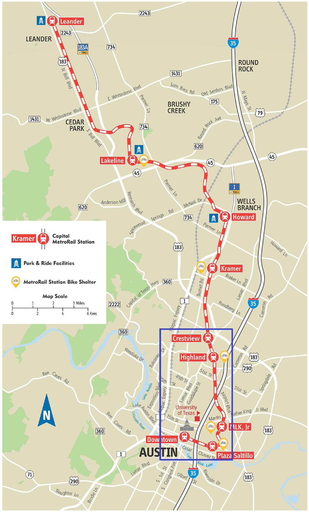
Current red transit line in Austin ( 29 ).

Austin Network

The year 2030 is considered for scenario runs in this analysis, with travel demand across a 3-mi × 6-mi square region in central Austin, and a more frequent transit service between Crestview Station and downtown Austin. Figure 2a indicates the network obtained from OSM and Figure 2c illustrates the network in the SUMO, which contains 11,025 nodes and 25,919 links. The geographical extent of the study area is limited to five stations of the Red Line. Segments of Interstate-35 and Mopac freeways are included in the map to reflect a realistic route choice for road users. The network downloaded from OSM is cleaned and vetted so that there are no dead-end roads or invalid junctions. Signal settings for each intersection are left as default (provided by OSM), and rail trains have a higher right-of-way over vehicles running on the roadway. Reflecting real-world conditions, roadway vehicles will stop and let rail trains pass whenever the vehicles and trains approach a shared intersection. Though rail connections are bidirectional in the real world, SUMO is not capable of simulating bidirectional railway lines and operation. Therefore, two commuter rail lines are coded (one for each direction), with separate platforms created for the rail line in each direction. SAVs drop SAV-and-ride users at the curb nearest to the railway station, and the pedestrian will walk the rest of the way to get the platform of the commuter rail line to access the rail train. Similar modeling is used to represent pick-ups of SAV-and-ride users.

Figure 2.

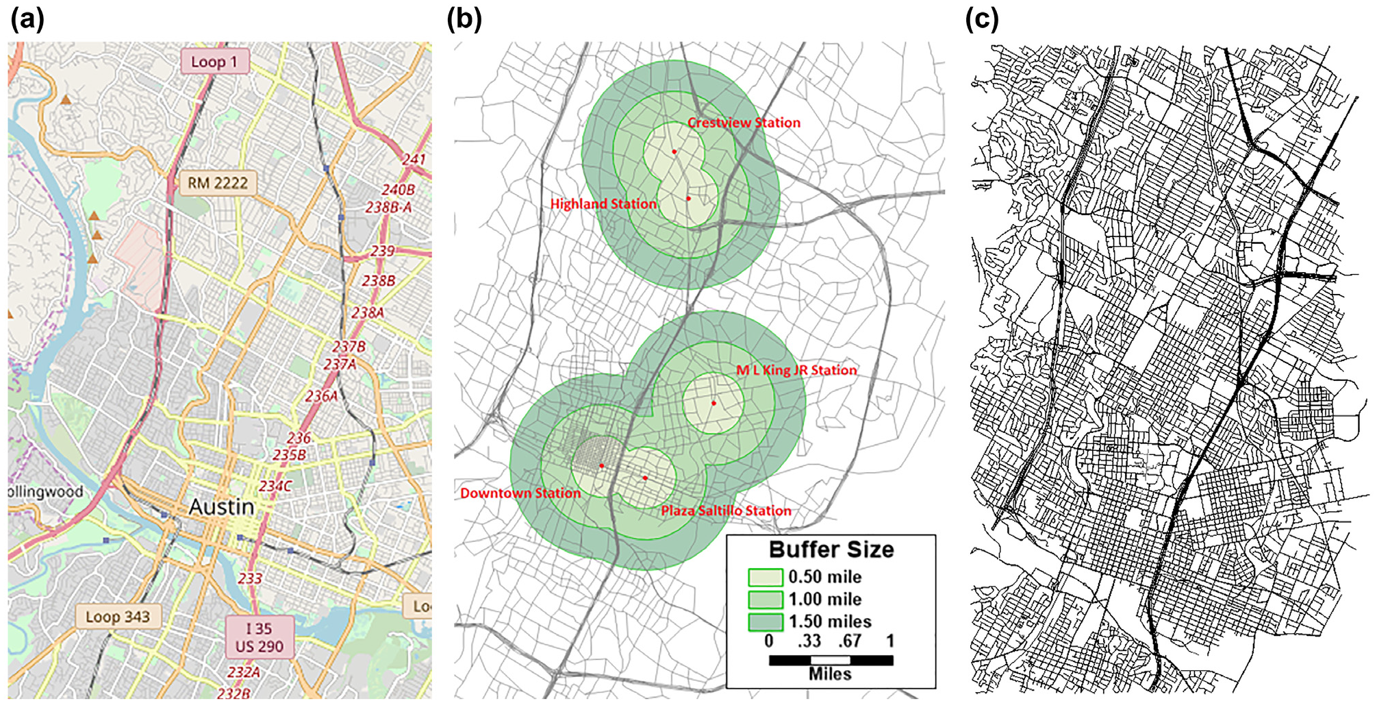
Network and automated mobility districts boundary in Austin: (a) Network from OpenStreetMap, (b) Road network from CAMPO with buffer area, and (c) SUMO simulation network.

AMDs are usually identified as neighborhoods or districts with a high density of trips, such as a university campus, central business districts, or a military base ( 8 ). In this study, a buffer from a station is considered as the operational extent of the SAVs. Buffer size is limited to 1.5 mi to avoid the excessive overlap between AMDs. In that case, the areas of five rail stations with buffers become two AMDs, as shown in Figure 2b. Each AMD has an SAV fleet that provides on-demand FMLM connections to transit trips in the corresponding AMD network. The first AMD contains two stations: Crestview Station and Highland Station, whereas the second AMD contains three stations: MLK Station, Plaza Saltillo Station, and Downtown Station. Furthermore, 0.25 to 0.5 mi is often seen as the walking distance to transit stations ( 30 ), so the maximum buffer for accessing and egressing from stations by walking is set as 0.5 mi (0.5-mi radius, as shown in Figure 2b).

Travel Demand

Travel demand used in this study reflects the demand forecasted for year 2030 by the CAMPO regional travel demand model. The CAMPO model has 2,252 traffic analysis zones (TAZs) covering Austin’s six-county region. Travel demand between origin–destination (OD) pairs from 246 TAZs was extracted from the CAMPO model for this study. As the network was obtained from OSM, a many-to-one association was established between the OSM links and the CAMPO TAZ boundaries. Based on CAMPO’s OD trip table, every trip was reformatted into an edge-based OD table where the origin edge and destination edge were randomly selected from links associated with the corresponding TAZs. The morning peak period (6–9 a.m.) was used as the simulation horizon. Departure times from each TAZ were randomized using a normal distribution across the simulation time horizon. There were 40,771 trips generated across the 246 TAZ regions during the morning peak period: from 6 a.m. to 9 a.m. In this exercise, mode choice was conducted on the whole morning peak demand set, and a 10% sample (4,077 trips) was simulated to reflect a certain level of congestion and avoid excessive micro-simulation run times.

Methodology

Simulation Framework

The simulation exercise in this effort was carried out using SUMO, which is an open-source, microscopic, and multimodal traffic simulation software package ( 13 ). Using SUMO, it is possible to carry out micro-simulations of multimodal vehicles considering the effects of traffic signals, vehicle routes, and driving behavior models. Multimodal microscopic functions make SUMO a tool that can explicitly model the interactions among pedestrians, SAVs and transit (e.g., access and egress of transit use), getting on and off the SAVs, and ride-sharing mechanisms for on-demand services.

TraCI (Traffic Control Interface) is an application programming interface tool in SUMO that allows for the retrieval of values of simulated objects and for the manipulation of their behavior “on-line” ( 13 ). On-demand services in SUMO can be implemented through TraCI by retrieving the information of on-demand requests and then dispatching vehicles to serve the demand (pick-up and drop-off). On-demand service has been tested on a small AMD (1,364 edges and 570 nodes) in Greenville, South Carolina, with about 300 trips served by a fleet of four on-demand vehicles and two fixed-route vehicles ( 9 ). This study builds on previous efforts by Zhu et al. ( 9 ) by incorporating interactions between pedestrians, SAVs and transit, and by implementing SAVs as an FMLM connection to a larger transit line.

Figure 3 shows the details of the whole simulation with feedbacks on waiting time and transit’s access and egress travel time. The SUMO simulation routine started with data preparation, and by reading travel demand, road network data, and configurations of FMLM service. Demand data include trips (derived from the OD trip table as described above) along with departure time. Network data comprise all the roadway links, transit lines, curbs, and platforms. Transit was coded as a high-capacity commuter rail running from Crestview Station to downtown, and back to its origin. The commuter rail runs with a headway of 15 min and a stop duration of 30 s at each station. SAVs have a capacity of three riders, an acceleration of 4.82 ft/s², deceleration of 6.56 ft/s², and an emergency deceleration of 24.61 ft/s² ( 31 , 32 ).

Figure 3.

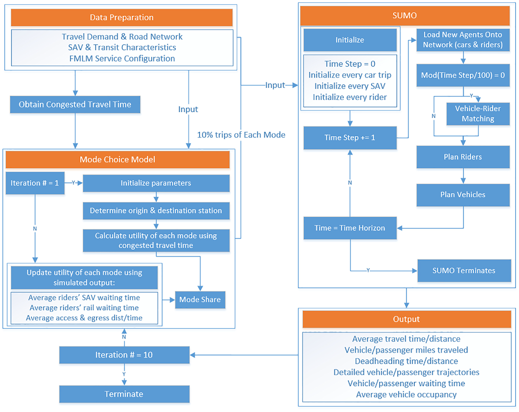
Simulation framework.

For this simulation study, travelers are given a choice spectrum comprising four modes: walking, private automobile (also referred to as car travel), walk-and-ride transit, and SAV-and-ride transit. Mode splits were determined based on mobility characteristics of each mode (such as wait time and in-vehicle travel time). Before the first iteration, a complete iterative run assuming all travelers using car mode was conducted to estimate congested travel times. For the first iteration, routes for walk, car, and walk-and-ride modes were determined based on shortest paths measured using those congested travel times in SUMO, and the origin and destination station for transit mode (Walk-and-ride and SAV-and-ride) were calculated for rest of the simulation. As there is a feedback in the mode choice from one iteration to the next, simulated riders’ waiting time for SAVs and trains, and average access and egress time were then used to update the utility of each mode and thus the mode share for the next iteration. Although mode choice was estimated for all travelers, only 10% of those trips were randomly selected for SUMO simulation.

Vehicles and persons were simulated on a second-by-second basis. SUMO starts by setting the current time step as ‘0’ (zero) and reading the trip information from mode choice, so it is aware of when to insert cars, walkers, and riders into the simulation. SAVs are initialized on roads at time 0 and wait for requests. Pedestrian and car mode users follow the assigned route plan, whereas SAV-and-ride users make a request and wait for the shuttle to pick them up (at their origin location or the transit station). Every 100s, SAVs evaluate requests from passengers and generate a plan that picks up the passengers and drops them off based on their trip request times. An SAV-and-ride user’s trip consists of the following segments: making an on-demand request at the origin, getting on and off an SAV, walking to the transit station, waiting at the origin transit station and taking transit to the destination station, walking out of the station and making another on-demand request, getting on and off an SAV, and walking to the final destination. For the analysis presented in this paper, mode of access and egress is assumed to be the same, meaning that walking from origin location to transit station, and taking an SAV at destination station is not allowed. The authors acknowledge that this is an important limitation, and plan to address this in future research efforts. Access- and egress-walking distance is limited to 0.5 mi around the station, and SAV fleets serve only in the AMDs designated to them (i.e., SAVs designated to serve the Downtown-Plaza-ML King Jr AMD will not honor trip requests from the Crestview-Highland station AMD).

At the end of the simulation routine, SUMO outputs second-by-second vehicle traces, as well as ride-sharing plans, which helps in computing performance metrics for various modes used in the next iteration. Because of the computation complexity of the problem, the whole simulation terminates when the tenth iteration concludes, to reach a small waiting time difference (less than 5%) between the last two iterations for all tested scenarios (including sensitivity analysis).

Mode Choice

Mode choice decisions are modeled at the trip level, using a nested logit model ( 33 ). SUMO-generated network travel times and wait time information was used to calculate mode shares. The two-level nested logit model considered walk-and-ride and SAV-and-ride nested under transit mode, which was compared with walk and drive at the same level (shown in Figure 4). Parameters and their coefficients in the mode choice model are adapted from relevant literature ( 20 , 34 ) with some necessary adjustments and assumptions. Value of in-vehicle travel time (IVTT) for car mode is set as $17.67 per hour, following Liu et al. ( 20 ). Value of out-of-vehicle travel time (OVTT), comprising wait and walk times, is assumed to be twice as much as the value of IVTT. The same value of OVTT is used for all modes, knowing that different modes will have different configurations of wait and walk times. For example, walk mode will not have any wait time associated with it as an individual simply walks from origin to destination. Car mode is assumed to provide door-to-door connectivity, so it does not have wait or walk time components. For SAV-to-ride, the value of OVTT parameter consists of wait time (for SAV at the origin), walking and waiting time for transit, as well as walking and waiting for an SAV at the transit station. The operating cost of private car (or light-duty vehicle) mode is assumed to be 60 cents per mile, whereas transit has a $2 flat fee ( 20 ). The distance coefficient was obtained from Wen et al. ( 19 ) and the alternative-specific constant for car mode utility was calibrated to be –10.3, to align with CAMPO’s mode shared estimates ( 35 ).

Figure 4.

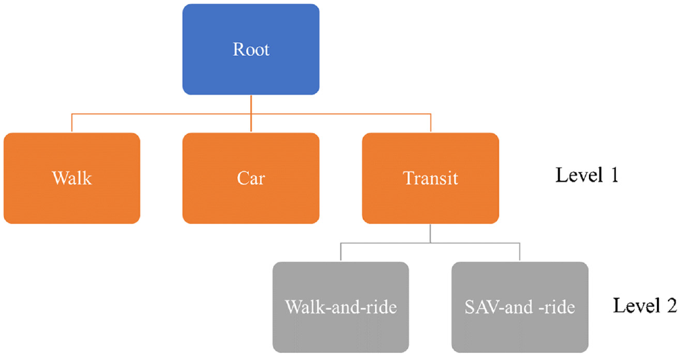
Two-level mode choice structure.

Walking mode utility does not change after the first iteration, to assume an unchanged behavior and save computation time. Assuming a walking speed of 3.1 mph ( 36 ), the utility of walking mode is:

V_{walk} = - 1.2 \times d_{walk} - 35.34 \times t_{walk}

where $d_{walk}$ is the walking distance in miles and $t_{walk}$ is the walking time in hours. Car mode uses driving distance and congested travel from the pre-run and the utility is:

V_{car} = - 10.3 - 0.6 \times d_{driving} - 17.67 \times t_{driving}

The transit utility function calculation is a bit more involved compared with that of other modes. First, the transit stations closest to a trip’s origin and destination locations must be identified by examining the shortest Euclidean distance. If the same station is the closest one to both the origin and the destination (i.e., in the case of short trips), transit mode is precluded from the choice set. As an SAV operates within a designated AMD, the SAV-and-ride mode is not considered a feasible mode if the Euclidean distance from a trip’s origin location to a transit station is greater than 1.5 mi (radius of an AMD). For walk-and-ride mode, if the Euclidean distance to the access- or egress-station is greater than 0.5 mi, the walk-and-ride mode is removed from the available mode set, as distance threshold for walk mode is set at 0.5 mi ( 30 ). The transit travel distance is computed as the railway distance between the platform centroid points of the boarding and alighting stations. The average speed of urban rail systems in the U.S. is observed ranging between 19 and 38 mph ( 37 ). So, the maximum speed of transit mode is set to be 32 mph and not affected by congestion on the roadway. The maximum vehicle speed of SAVs is set at 30 mph, because the running speed of current demonstrated automated shuttles lies between 15 mph and 30 mph ( 6 ).

Value of IVTT for both modes nested under transit is assumed to be half of car mode ( 20 ). Walk time for accessing and egressing transit (i.e., $t_{{access}_{walk}}, t_{egres s_{walk}}$ ) is calculated based on the network’s shortest distance path for each person. For the first iteration, waiting time for rail ( $t_{waiting}$ ) is assumed to be half of the transit headway, both for walk-and-ride and SAV-and-ride modes. For the iterations afterward, the waiting times for rail are extracted from previous iterations and updated using the method of successive average (MSA). Using the superscript n for the index of feedback iteration n, the average waiting time for rail can be expressed as:

t_{waiting}^{n + 1} = \frac{n - 1}{n} t_{waiting}^{n - 1} + \frac{1}{n} t_{waiting}^{n}

After obtaining the locations of the origin and destination stations, the utility of walk-and-ride mode can be computed using:

V_{w & r} = - 2 - 8.84 \times t_{rail} - 35.34 \times (t_{acces s_{walk}} + t_{egres s_{walk}}) - 35.34 \times t_{waiting}

Waiting time for SAVs for both first-mile and last-mile (i.e., $t_{FM - waitin g_{SAV}}, t_{LM - waitin g_{SAV}}$ ) is assumed to be 2.5 min in the first iteration, but will be updated using MSA in the following iteration based on the simulated average waiting time.

First-mile SAV travel distance ( $d_{F M_{SAV}}$ ) used in SAV-and-ride utility for each traveler is assumed to be the congested network travel distance from origin to station; however, it is computationally expensive to track and update the travel distance of each passenger for every iteration. This metric is calculated using congested network travel distance from origin to station for the first iteration ( $d_{F M_{SAV}}^{1}$ ), but is approximated via expanding (or shrinking) the first-iteration distance by a factor K for the iteration afterward ( $d_{F M_{SAV}}^{n}$ , $n \geq 2$ ). The factor K is the ratio of the modified simulated average first-mile distance ( $D_{F M_{avg}}^{n}$ ) across all SAV-and-rider users to the average first-mile distance in the first iteration ( $d_{F M_{avg}}$ ) across all SAV-and-ride users:

d_{F M_{SAV}}^{n + 1} = d_{F M_{SAV}}^{1} * (\frac{D_{F M_{avg}}^{n}}{d_{F M_{avg}}})

where the modified simulated average first-mile distance index is calculated based on the simulated average first-mile travel distance ( $d_{F M_{avg}}^{n}$ ) of the two most recent iterations, using MSA:

D_{F M_{avg}}^{n} = \frac{n - 1}{n} d_{F M_{avg}}^{n - 1} + \frac{1}{n} d_{F M_{avg}}^{n} (n \geq 2)

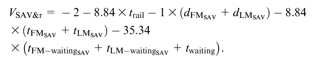
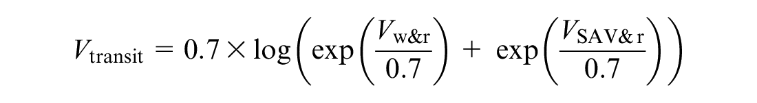
Similar calculations are conducted to deal with last-mile SAV travel distance ( $d_{L M_{SAV}}$ ), as well as first-mile and last-mile SAV travel time $(t_{F M_{SAV}} and t_{L M_{SAV}})$ . Assuming the operating cost of an SAV is $1/mile ( 20 ), the utility of SAV-and-ride comes out to be:

\begin{matrix} V_{SAV & r} = - 2 - 8.84 \times t_{rail} - 1 \times (d_{F M_{SAV}} + d_{L M_{SAV}}) - 8.84 \\ \times (t_{F M_{SAV}} + t_{L M_{SAV}}) - 35.34 \\ \times (t_{FM - waitin g_{SAV}} + t_{LM - waitin g_{SAV}} + t_{waiting}) . \end{matrix}

The nesting coefficient for transit is set as 0.7 based on the mode choice component of the CAMPO travel demand model ( 38 ); therefore, the utility of transit is:

V_{transit} = 0.7 \times \log (\exp (\frac{V_{w & r}}{0.7}) + \exp (\frac{V_{SAV & r}}{0.7}))

Based on the utility equations shown above, mode shares are computed for all modes. Mode share changes when entering a new iteration based on the information from the previous iteration.

Real-Time Simulation Control of SAVs and Passengers

The real-time simulation control primarily focuses on passenger and SAV movements for the transit riders choosing the SAV-and-ride option. At each time step (i.e., every 1 s), SAV-and ride transit users are tagged with different flags so that the simulation controller can obtain and react to a riders’ current status and location. SAV ride requests from passengers are evaluated every 100 s. Armed with information on passengers’ pick-up and drop-off locations, routing plans are generated for each vehicle in the SAV fleet to pick up and drop off passengers based on the order of their trip request. A naïve logic was implemented in the preliminary analysis and will be enhanced with dynamic ride-sharing functionalities in future research (such as en-route adjustments to pick up additional passengers).

From the rider perspective, Figure 5 gives an example of two SAV-and-ride users. Ben (marked in blue) chose to travel from home to work by taking transit from station 1 to station 3, and Jerry (marked in green) chose to travel from home to a shopping location, by taking transit from station 2 to station 3. First, Ben and Jerry both walked to the street where they can be picked up by an SAV. As station 1 and station 2 are in AMD 1, a yellow SAV serving AMD 1 was assigned to pick up and drop off Ben and Jerry at their respective transit stops. The yellow SAV made an empty-vehicle trip to pick up Ben, and then proceeded along to pick up Jerry. The SAV then traveled to station 1 to drop off Ben (as he was picked up first and this was his selected origin station), and then dropped off Jerry at his selected origin station (#2). After dropping all the passengers off, the yellow SAV was re-located to a nearby location on the network where it can park itself and wait for the next trip request. Ben and Jerry walked to the station and waited for the train. Once the train arrived, Ben and Jerry boarded the train at their respective stations and got off the train at station 3. Both Ben and Jerry walked out of the station to be picked up by an SAV. As station 3 is in AMD 2, an orange SAV serving AMD 2 was then assigned to pick Ben and Jerry up. Following the same ride-sharing logic, Ben and Jerry walked to their destination locations after being dropped off by the SAV. The orange SAV was re-located in a similar fashion as described for the yellow SAV.

Figure 5.

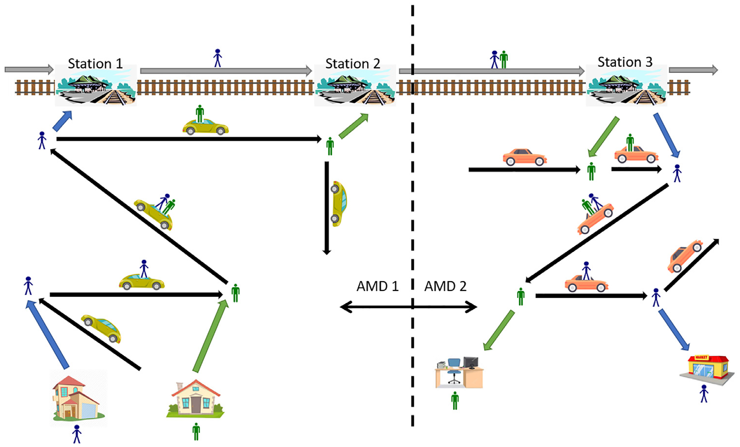
Example flow of two SAV-and-ride users and their SAV movement.

The various stages in SAV-and-ride operation are described in detail below. The terms transit rider, user, and SAV-and-ride user are used interchangeably in the description.

Stage 0: Initialization. Information in relation to origin edge, first-mile SAV pick-up edge, first-mile SAV drop-off edge, and origin transit station is identified for each SAV-and-ride user. At this stage, an SAV-and-ride user commences walking to the network edge where they will be picked up.

Stage 1: SAV-and-ride user arrives at first-mile departure location (random point of the pick-up roadway link) and waits for a ride. Any SAV-and-ride user arriving at a departure location will be assigned with an SAV at the next vehicle re-plan step (i.e., the next 100 s time bin).

Stage 2: SAV-and-ride user boards the vehicle and the SAV proceeds to pick up the next user assigned to it. If all the seats on the SAV are occupied or when there are no more passenger pick-up requests (in a given time step), then the SAV heads to drop off the passengers.

Stage 3: When the SAV has picked up all assigned SAV-and-ride transit users, the users’ stage will be changed to stage 3. The SAV will drop off all the passengers at their designated station locations.

Stage 4: SAV-and-ride user has been dropped off at the transit station and commences walking to the origin transit station platform. There is a walking leg involved here, as transit riders cannot be dropped by the SAVs directly on the transit platform.

Stage 5: SAV-and-ride user arrives at the origin station and waits for the train. Once a user reaches this stage, the rest of his/her journey will be identified and cached, including destination transit station, last-mile SAV pick-up edge, last-mile SAV drop-off edge, and final destination edge.

Stage 6: Once the train arrives at the station, the rider will board the train.

Stage 7: The SAV-and-ride user has been dropped off at the destination station and walks to the location where he/she will be picked up by an SAV.

Stage 8–11: These stages represent the SAV routing logic for the last mile, as described in stages 1–3.

Stage 12: SAV-and-ride user arrives at the final destination edge.

The SAVs are controlled using TraCI module in SUMO, constantly reacting to the status of the SAV-and-ride transit users. Various stages in SAV operations are described below:

Stage 0: Initialization. SAVs are placed at random locations in their designated AMDs.

Stage 1: Idling. Before receiving a request (evaluated every 100 s), SAVs are parked, and wait for a trip request.

Stage 2: Routing and running. Once a routing plan is generated for an SAV to pick up and drop off riders, it will proceed to the first pick-up point. Each SAV will first pick up all the passengers assigned to it on a trip, and then drop off the passengers in the sequence they were picked up. If the vehicles are all occupied by passengers, the remaining riders will not be served during this re-plan step. They will have the priority to be assigned an SAV at the next re-plan step (after 100 s). During the waiting process, riders are not able to shift travel mode, which has been defined before SUMO starts.

Stage 3: Redistribute. After an SAV has finished dropping off all passengers, it is re-located to a nearby location on the network where it can park itself and wait for the next trip request (reflecting a real-world situation where ride-hail drivers often relocate themselves to a location in anticipation of future trip demand).

Austin Application Results

Baseline Scenario Versus FMLM Scenario

For the Austin case study, the baseline scenario only considers walk, drive, and walk-and-ride modes as the modal alternatives. Transit is assumed to be running between Crestview Station and downtown Austin with a headway of 15 min in the baseline (as well as FMLM) scenario. The FMLM scenario is tested with each AMD served by a fleet of 15 SAVs, which has been tested to deliver a reasonable average wait time (under 5 min) for SAVs. Table 1 shows the mode share results for the baseline scenario as well as the FMLM scenario. Both scenarios run with 4,077 trips, which is 10% of the total morning peak travel demand for the defined region.

Table 1.

Comparison results of the base case and FMLM served by SAVs

	Mode share				Average vehicle occupancy	1,000 VMT(10% of AM peak travel demand)
Scenarios	Car	SAV & Ride	Walk & Ride	Walk	Average vehicle occupancy	Car	SAV	Empty	Total
Base	91.1%	0%	0.35%	8.52%	1.00	14.0	0	0	14.0
Base	37,153 trips	0	143	3,475	1.00	14.0	0	0	14.0
FMLM	87.4%	3.71%	0.35%	8.53%	0.74	13.1	1.0	0.5	14.7
	35,639 trips	1,514	141	3,477	0.74	13.1	1.0	0.5	14.7
	On-board time (min per person)		Wait time (min per person)		Walking time (min per person)		Travel distance (miles per person)		Total time (min per person)
	SAV^*	Transit	SAV	Transit	SAV	Transit	SAV	Transit
	7.0	14.4	6.8	7.6	3.8	3.8	2.04	1.93	43.3

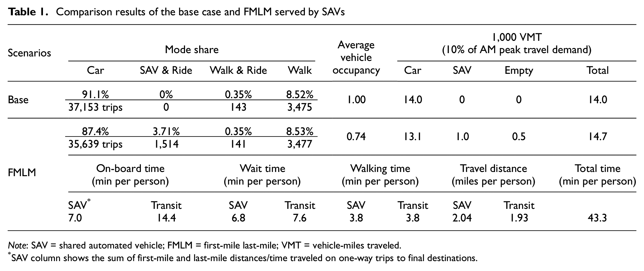
Note: SAV = shared automated vehicle; FMLM = first-mile last-mile; VMT = vehicle-miles traveled.

SAV column shows the sum of first-mile and last-mile distances/time traveled on one-way trips to final destinations.

A transit survey conducted in Austin in 2011 shows a total of 1,755 daily transit trips for the rail line across all stops ( 38 ). As this paper simulated 10% of total demand, the analysis would capture 176 trips spread across all the nine stations. Further assuming that these boarding trips are distributed uniformly across all stations, 78 daily transit trips would be captured in the five stations investigated in this paper (among nine stations that have been built currently), across the whole day. Therefore, 14 trips during the a.m. peak for walk-and-ride mode align reasonably well with the 2011 field observation. Further, the CAMPO model shows a walking mode share of 4% across Austin’s 6-county region, whereas the baseline scenario estimated a walking mode share of 8.5%, which is reasonable for central Austin, where walking is more likely to happen. The baseline scenario also provides a car mode share of 91.1%, which aligns well with CAMPO’s 92.0% prediction.

Share of walk-and-ride, as well as walking, remains almost unchanged between the baseline scenario and the FMLM scenario. The 0.5-mi constraint on walking to transit might play a part in keeping the mode share for walk-and-ride constant. For the FMLM scenario using 15 vehicles serving each AMD under a rail headway of 15 min, SAV-and-ride mode gains mode share from car, about 1,514 trips, which accounts for 3.71% of the total demand. The reasons for this could be cost- and time-effectiveness of SAV mode, compared with car mode. The use of transit increased from 0.35% to 4.06% when SAV is introduced, which is an increase of more than 10 times. As the access and egress mode is assumed to be the same, 30 SAVs (with 15 in each AMD) in this 10% morning peak travel demand scenario can serve 302 person-trips in total, about 10 person-trips served by each SAV during the 3-h morning peak.

Although SAV modes gain mode share, the average occupancy of all vehicles dropped to 0.74 persons in the FMLM simulation, from 1 in the baseline. The primary reason for this is the empty-vehicle travel encumbered by SAVs both in traveling to pick up the first passenger, as well as in relocating after dropping off the last passenger. Empty-vehicle travel accounts for 48% of SAV VMT (and 3.4% of total VMT), which is in close alignment with deadhead miles quantified using real-world TNC data ( 39 ). The naïve ride-matching and routing logic used for preliminary analysis may also be a reason for the SAV empty VMT observed here. Based on this logic, SAVs always pick up passengers in the order of their requests, and drop off in the order of their pick-ups (as opposed to geographical proximity to the shuttle location). A positive result from the deployment of SAVs in AMDs is that car VMT has seen a reduction of 6.4% (from 14,028 to 13,149), although using SAVs increases the total VMT by 5%. This could reduce congestion on the highway and increase travel speeds, but could lead to increased congestion at local places around transit stations.

When rail trains come every 15 min and 15 SAVs serve in each AMD, the average total travel time per passenger for SAV-and-ride mode is 41.4 min, which consists of riders’ travel time on both SAVs and rail, wait time for SAVs and rail, and the walking time from the edge outside the station to the railway platform and from the railway platform to the edge outside the station. Average waiting time for an SAV trip (either FM or LM) is 3.4 min, with 3.5 min of average on-board time. Although the maximum speed of the railway is 32 mph, the results show an average speed of 8.0 mph when riders are on board, because of the train frequently stopping and waiting at each station. A person’s wait time for transit is close to half of the transit headway, which could be a uniform-distributed arrival at the train station.

Sensitivity Analysis

After exploring the impacts of implementing SAVs as a modal alternative to car and walk-and-ride modes, sensitivity analysis exercises (see Table 2) were carried out to understand the impact of fleet size and transit frequency on the performance of the SAV mode. The FMLM scenario presented above has a transit headway of 15 min and a 15-vehicle fleet in each of the two AMDs (30 vehicles total). Building on this, scenarios were developed to test the performance of the SAV-and-ride mode, based on transit frequencies of 5 min, 10 min, 15 min, and 20 min, and increasing SAV fleet size in each AMD from five to 20 vehicles (in increments of five vehicles).

Table 2.

Sensitivity analysis of transit frequency and fleet size

	Mode share				Average vehicle occupancy	1,000 VMT(10% of AM peak travel demand)
Scenarios	Car	SAV & ride	Walk & ride	Walk	Average vehicle occupancy	Car	SAV	Empty	Total
Base	91.1%	0.00%	0.35%	8.52%	1.00	14.0	na	na	14.0
Headway (minutes between trains)
5	85.3%	5.78%	0.36%	8.51%	0.92	12.8	1.6	0.7	15.1
10	86.6%	4.48%	0.36%	8.52%	0.83	13.1	1.2	0.5	14.9
15	87.4%	3.71%	0.35%	8.53%	0.74	13.1	1.0	0.5	14.7
20	88.9%	2.25%	0.33%	8.55%	0.69	13.3	0.6	0.3	14.2
Fleet size (#SAVs in each AMD)
5	90.2%	0.89%	0.35%	8.53%	0.43	13.1	0.3	0.2	13.6
10	88.7%	2.42%	0.35%	8.53%	0.64	13.0	0.7	0.3	14.0
15	87.4%	3.71%	0.35%	8.53%	0.74	13.1	1.0	0.5	14.7
20	85.3%	5.86%	0.35%	8.53%	0.82	12.3	1.6	0.8	14.7
	On-board time (minutes per person)		Wait time (minutes per person)		Walking time (minutes per person)		Travel distance (miles per person)		Total time(min per person)
Scenarios	SAV^*	Transit	SAV	Transit	SAV	Transit	SAV	Transit	Total time(min per person)
Headway (minutes between trains)
5	10.3	13.8	10.5	2.5	3.8	4.7	3.17	1.78	45.6
10	8.9	13.7	9.2	5.1	3.8	5.3	2.80	1.95	46.0
15	7.0	14.4	6.8	7.6	3.8	3.8	2.04	1.93	43.3
20	6.5	14.2	6.5	10.0	3.7	3.8	1.99	2.02	44.7
Fleet size (#SAVs in each AMD)
5	5.5	15.1	7.3	7.0	4.0	4.3	1.46	2.39	43.3
10	7.0	16.1	7.2	7.4	3.7	4.4	2.04	2.18	45.7
15	7.0	14.4	6.8	7.6	3.8	3.8	2.04	1.93	43.3
20	7.1	16.9	6.4	7.5	3.6	5.5	2.13	2.44	47.0

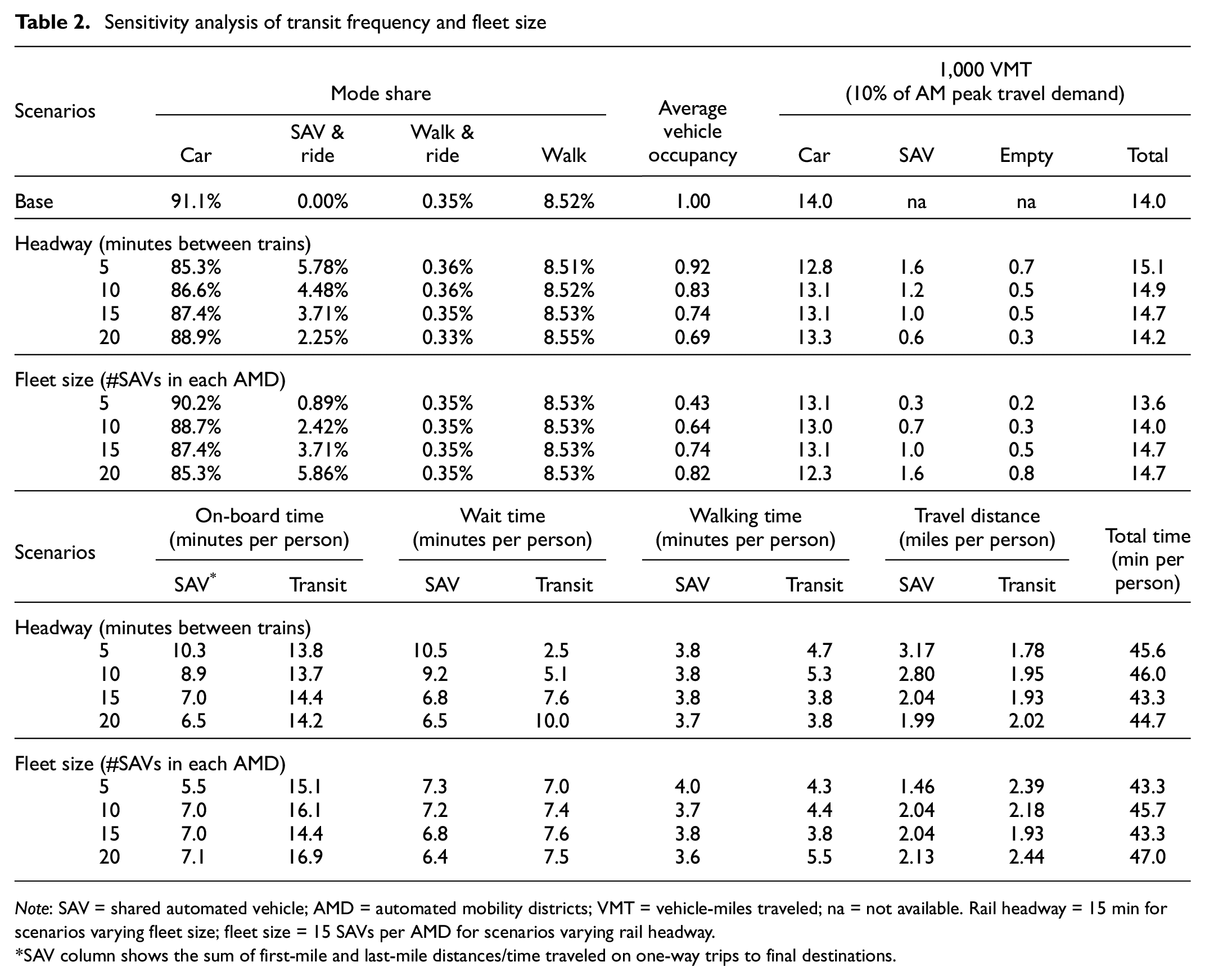
Note: SAV = shared automated vehicle; AMD = automated mobility districts; VMT = vehicle-miles traveled; na = not available. Rail headway = 15 min for scenarios varying fleet size; fleet size = 15 SAVs per AMD for scenarios varying rail headway.

SAV column shows the sum of first-mile and last-mile distances/time traveled on one-way trips to final destinations.

With a more frequent transit service, the SAV-and-ride mode took a larger mode share, up to 5.78%, about 225 trips (450 person-trips by SAVs) among 10% of the morning peak travel demand. This means the SAVs were utilized more when the transit service was frequent, as also shown in the increased average vehicle occupancy as well as more VMT by SAVs and fewer VMT by cars. Further, SAV on-board time, wait time, and average trip length per person also increased as the headway decreased, as a result of more shared rides, because SAVs would pick up and drop off more passengers in one routing plan, which led to longer wait times for the second and third passengers. Wait time for transit saw a significant reduction when transit service frequency increased, as expected. However, the total time remained similar (about 45 min) among the four scenarios varying the railway headway, showing that people are more concerned with the total travel time when deciding the mode to use: if the transit service is frequent, they are more willing to wait longer for an SAV. As only central Austin was simulated, the average transit distance per person showed a slightly increasing trend, possibly because of the people who are likely to take the SAV-and-ride mode when the transit service is frequent despite the short transit distance. However, one may see a clear pattern when the simulation can be extended to Austin’s six-county region. Walking time is also quite stable among the scenarios (within 4 min for summed walking time for FM and LM, and within 4 min from the SAV’s drop-off edge to platform), with some fluctuations in transit wait time, owing to different lengths of the railway platforms.

A larger fleet size led to a higher mode share of SAV-and-ride, mostly because of the increased SAV service accessibility. The SAVs were utilized more under a large fleet size, since a small fleet size was not enough to provide the desired level of service and people moved away from the SAV-and-ride mode. As expected, a larger fleet size would lead to more VMT by SAVs, and the empty VMT remained approximately 48% of all VMT driven by SAVs. A larger fleet size led to shorter wait times, but total travel times among fleet size scenarios were quite stable, meaning that fleet size would not affect the riders’ door-to-door travel time too much. Smaller SAV fleet sizes are not enough to accommodate riders’ requests and lead to a smaller mode share for SAVs serving the rail stations, along with shorter-distance rides, and longer wait times, on average.

Discussion

When the simulation is expanded include to all morning peak demand, more SAVs are needed to serve Austin’s rail-transit connections. Results will also be affected by the use of larger SAVs (e.g., vans and minibuses), less demand-responsive routing of SAVs, and longer SAV-to-rider matching periods (e.g., 100 s rather than 1 s used here). Such shifts can create greater efficiencies but depend on the density of demand in time and space, and willingness of travelers to call ahead or walk to pick-up points.

Other researchers’ mesoscopic simulations of SAV fleet operations almost uniformly neglect FMLM services, including walk access details, transit facility geometries, and traffic impacts of idling SAVs (during curbside pick-up and drop-offs, for example). This paper’s use of SUMO for SAV and FMLM micro-simulations can more realistically reflect such behaviors, though computing times and scale of demonstration remain an issue. Although some mesoscopic simulators are capable of simulating millions of distinct agents over a typical travel day ( 40 ), high-performance computers are required, and computation times are not short. For a look at FMLM behaviors around transit stations, the SUMO micro-simulation used here is a good choice.

Conclusion

Extending the concept of deploying SAVs in geofenced regions with a high trip density (labeled as an Automated Mobility District, or an AMD), this paper explores the idea of using SAVs to provide FMLM connectivity to transit in AMDs. Although there are some mesoscopic agent-based simulations on transit, transit operations are oversimplified and FMLM service is rarely investigated. This paper makes one of the first attempts at understanding the scope for adopting SAVs for FMLM connections using the microscopic simulation tool SUMO. This paper not only models detailed transit operations (such as stopping duration, schedule, shared intersections by railway and roadway, and railway platforms for getting on and off) but also makes a foray into incorporating operational logic associated with deploying SAVs for FMLM connections to transit. Outputs from the micro-simulation represent second-by-second passenger and vehicle movements, which can be used to obtain accurate estimates of VMT, energy and fuel consumption, and performance metrics for the SAV mode (e.g., ride-sharing time, walking time, and waiting time). Furthermore, this paper extends the AMD concept to a larger network with multiple AMDs. With rising interest in SAV technology as an urban mobility solution, AMD deployments may become common (with SAVs providing FMLM services to transit stations, on demand).

This paper uses SAV fleets around Austin’s light-rail Red Line stations. For the study 10% percent of the region’s travel demand was evaluated and then micro-simulated using the open-source SUMO tool, augmented with a nested logit model for mode (and access-mode) choices. With SAVs serving FM or LM requests in their designated AMDs, an estimated 3.71% of current person-trip-making would shift from private-car modes to the SAV-and-ride mode, leading to 10 times increase in the use of transit with stable walk-and-ride mode share. SAV use raises systemwide VMT slightly, while lowering average vehicle occupancy slightly, owing primarily to SAVs’ empty-vehicle travel (between customers). As FMLM trips to rail stations are very directed in the a.m. peak period, 48% of the SAVs’ VMT was empty (no occupants), comprising 3.4% of total VMT in the 3 mi × 6 mi system. This calls for the development of deadhead minimization routines, to reduce empty VMT from SAVs and AVs. Using sensitivity testing across scenario settings, SAVs were utilized more when train service was more frequent. Lower train headways also lowered SAV on-board time, wait time, and average trip length. Mode choice in using SAVs for FMLM connections increased with more frequent transit service and larger fleet size, but total travel time served as the biggest determinant in trip-makers’ mode choices. Average walking times were quite stable across scenarios, at most 4 min for both SAVs and transit. Total (door-to-door) travel times were also quite stable across SAV fleet size scenarios.

Although this paper makes an initial attempt at simulating SAVs as an FMLM connection to transit, a few shortcomings remain to be addressed. It was observed that the naïve ride-matching and routing logic implemented in this study led to increased empty-vehicle travel in the system. Immediate efforts will focus on enhancing operational logic with features such as dynamic ride-sharing and deadhead minimization. The mode choice model would be more realistic if the parameters were calibrated by collecting the data via a stated preference survey. Time reliability can also be increased by enhancing the operating strategy of the SAV fleet as well as ride-sharing mechanisms. Access- and egress-legs to transit were enforced to be the same in the simulation for simplicity. This should be relaxed in the next iteration of this research, as transit riders in all likelihood could take an SAV to access a transit station but walk to the final destination for the egress-leg of the trip (or vice-versa). The results presented in this paper consider 10% of the demand for the region of interest, owing to the computational complexity of the micro-simulation. Solutions will be explored to simulate 100% of the AMD’s travel demand using advanced computing resources. One should also note that the use of SAVs to travel directly from origin to destination would, in reality, compete with using SAVs to provide FMLM service. Further effort should be made to incorporate SAVs serving the whole trip, as well as other FMLM modes (i.e., scooters and bikes) in the simulation.

Footnotes

Acknowledgements

This work was authored (in part) by the National Renewable Energy Laboratory, operated by Alliance for Sustainable Energy, LLC, for the U.S. Department of Energy (DOE) under Contract No. DE-AC36-08GO28308. The authors acknowledge Stan Young of NREL for leading the Urban Science Pillar of the SMART Mobility Laboratory Consortium. The following DOE Office of Energy Efficiency and Renewable Energy (EERE) managers played important roles in establishing the project concept, advancing implementation, and providing ongoing guidance: Prasad Gupte, Erin Boyd, Heather Croteau, and David Anderson. The authors also thank Jade (Maizy) Jeong for her excellent editing and submission support.

Author Contributions

The authors confirm contribution to the paper as follows: study conception and design: Y. Huang, K. Kockelman, V. Garikapati, L. Zhu; data collection: Y. Huang; analysis and interpretation of results: Y. Huang; draft manuscript preparation: Y. Huang, K. Kockelman, V. Garikapati, L. Zhu, S. Young. All authors reviewed the results and approved the final version of the manuscript.

Declaration of Conflicting Interests

The author(s) declared no potential conflicts of interest with respect to the research, authorship, and/or publication of this article.

Funding

The author(s) disclosed receipt of the following financial support for the research, authorship, and/or publication of this article: Funding was provided by the DOE Vehicle Technologies Office (VTO) under the Systems and Modeling for Accelerated Research in Transportation (SMART) Mobility Laboratory Consortium, an initiative of the Energy Efficient Mobility Systems (EEMS) Program.

The views expressed in the article do not necessarily represent the views of the DOE or the U.S. Government. The U.S. Government retains and the publisher, by accepting the article for publication, acknowledges that the U.S. Government retains a nonexclusive, paid-up, irrevocable, worldwide license to publish or reproduce the published form of this work, or allow others to do so, for U.S. Government purposes.

References

Bureau of Transportation Statistics. Commute Mode Share: 2015. U.S. Department of Transportation, Washington, D.C., 2016. https://www.bts.gov/content/commute-mode-share-2015.

Federal Transit Administration. 2018 National Transit Summaries and Trends: Office of Budget and Policy. U.S. Department of Transportation, Washington, D.C., 2019. https://cms7.fta.dot.gov/sites/fta.dot.gov/files/docs/ntd/data-product/134401/2018-ntst_1.pdf.

Loxton

O’Connor

Salman

Declining Bus Ridership: Improving the Efficiency of Transit Networks. McKinsey & Company, 2019. https://www.mckinsey.com/∼/media/McKinsey/Industries/CapitalProjectsandInfrastructure/OurInsights/DecliningbusridershipImprovingtheefficiencyoftransitnetworks/Declining-bus-ridership-Improving-the-efficiency-of-transit-networks.ashx.

Bösch

P. M.

Becker

Axhausen

K. W.

Cost-Based Analysis of Autonomous Mobility Services. Transport Policy, Vol. 64, 2018, pp. 76–91. https://doi.org/10.1016/j.tranpol.2017.09.005.

Loeb

Kockelman

K. M.

Liu

Shared Autonomous Electric Vehicle (SAEV) Operations across the Austin, Texas Network with Charging Infrastructure Decisions. Transportation Research Part C: Emerging Technologies, Vol. 89, 2018, pp. 222–233. https://doi.org/10.1016/j.trc.2018.01.019.

U.S. Department of Transportation. USDOT’s ITS JPO Evaluation Program. 2018. https://www.itsknowledgeresources.its.dot.gov/its/executivebriefings/2019/pdf/EB06-LOWSPEEDAUTOMATEDSHUTTLES_05_16_19_FINAL.pdf.

Ramsey

Autonomous Vehicles Fall into the Trough of Disillusionment ... But that’s Good. Forbes, 2018. https://www.forbes.com/sites/enroute/2018/08/14/autonomous-vehicles-fall-into-the-trough-of-disillusionment-but-thats-good/#69d493177b5a.

Hou

Young

S. E.

Garikapati

Chen

Zhu

Initial Assessment and Modeling Framework Development for Automated Mobility Districts. No. NREL/CP-5400-68290. National Renewable Energy Lab (NREL), Golden, CO, 2018.

Zhu

Garikapati

Chen

Hou

Aziz

H. M. A.

Young

Quantifying the Mobility and Energy Benefits of Automated Mobility Districts Using Microscopic Traffic Simulation. Proc., International Conference on Transportation and Development 2018: Connected and Autonomous Vehicles and Transportation Safety, American Society of Civil Engineers, Reston, VA, 2018, pp. 98–108. https://doi.org/10.1061/9780784481530.010.

10.

University of Michigan. Mcity Driverless Shuttle - A Case Study. 2018. https://mcity.umich.edu/wp-content/uploads/2018/09/mcity-driverless-shuttle-case-study.pdf.

11.

City of Arlington. Milo Pilot Program Closeout Report. Urbanism Next, University of Oregon, OR, 2017. https://www.urbanismnext.org/resources/milo-pilot-program-closeout-report.

12.

Smart Columbus. Self-Driving Shuttles. 2019. https://smart.columbus.gov/projects/self-driving-shuttles.

13.

Lopez

P. A.

Wiessner

Behrisch

Bieker-Walz

Erdmann

Flötteröd

Y.-P.

Hilbrich

Lucken

Rummel

Wagner

Microscopic Traffic Simulation Using SUMO. 2018 21st International Conference on Intelligent Transportation Systems (ITSC), Maui, HI, IEEE, New York, 2018, pp. 2575–2582.

14.

Shaheen

Chan

Mobility and the Sharing Economy: Potential to Facilitate the First-and Last-Mile Public Transit Connections. Built Environment, Vol. 42, No. 4, 2016, pp. 573–588.

15.

Yap

M. D.

Correia

van Arem

Preferences of Travellers for Using Automated Vehicles as Last Mile Public Transport of Multimodal Train Trips. Transportation Research Part A: Policy and Practice, Vol. 94, 2016, pp. 1–16. https://doi.org/10.1016/j.tra.2016.09.003.

16.

Delhi Metro Rail Corporation Ltd. Feeder Bus. 2017. http://www.delhimetrorail.com/feederbus.aspx.

17.

Fan

Ermagun

Cao

Wang

Das

Public Bicycle as a Feeder Mode to Rail Transit in China: The Role of Gender, Age, Income, Trip Purpose, and Bicycle Theft Experience. International Journal of Sustainable Transportation, Vol. 11, 2017, pp. 308–317.

18.

Pinto

H. K. R. F.

Hyland

M. F.

Mahmassani

H. S.

Verbas

I. Ö.

Joint Design of Multimodal Transit Networks and Shared Autonomous Mobility Fleets. Transportation Research Part C: Emerging Technologies, Vol. 113, 2020, pp. 2–20. https://doi.org/10.1016/j.trc.2019.06.010.

19.

Wen

Chen

Y. X.

Nassir

Zhao

Transit-Oriented Autonomous Vehicle Operation with Integrated Demand-Supply Interaction. Transportation Research Part C: Emerging Technologies, Vol. 97, 2018, pp. 216–234. https://doi.org/10.1016/j.trc.2018.10.018.

20.

Liu

Kockelman

K. M.

Boesch

P. M.

Ciari

Tracking a System of Shared Autonomous Vehicles across the Austin, Texas Network Using Agent-Based Simulation. Transportation, Vol. 44, No. 6, 2017, pp. 1261–1278. https://doi.org/10.1007/s11116-017-9811-1.

21.

Dandl

Bogenberger

Comparing Future Autonomous Electric Taxis with an Existing Free-Floating Carsharing System. IEEE Transactions on Intelligent Transportation Systems, Vol. 20, No. 6, 2018, pp. 2037–2047.

22.

Vosooghi

Puchinger

Jankovic

Vouillon

Shared Autonomous Vehicle Simulation and Service Design. Transportation Research Part C: Emerging Technologies, Vol. 107, 2019, pp. 15–33. https://doi.org/10.1016/j.trc.2019.08.006.

23.

Hörl

Balac

Axhausen

K. W.

Dynamic Demand Estimation for an AMoD System in Paris. Proc., 2019 IEEE Intelligent Vehicles Symposium (IV), Paris, France, IEEE, New York, 2019, pp. 260–266.

24.

Gurumurthy

K. M.

Kockelman

K. M.

Simoni

M. D.

Benefits and Costs of Ride-Sharing in Shared Automated Vehicles across Austin, Texas: Opportunities for Congestion Pricing. Transportation Research Record: Journal of the Transportation Research Board, 2019. 2673: 548–556.

25.

Alemi

Rodier

Simulation of Ridesourcing Using Agent-Based Demand and Supply Models Regional: Potential Market Demand for First Mile Transit Travel and Reduction in Vehicle Miles Traveled in the San Francisco Bay Area. eScholarship, 2018. https://escholarship.org/uc/item/3h1550wm.

26.

Shen

Zhao

Impact of Built Environment on First-and Last-Mile Travel Mode Choice. Transportation Research Record: Journal of the Transportation Research Board, 2018. 2672: 40–51.

27.

Haklay

Weber

OpenStreetMap: User-Generated Street Maps. IEEE Pervasive Computing, Vol. 7, 2008, pp. 12–18.

28.

Capital Area Metropolitan Planning Organization. 2005 Base Year Travel Demand Model Calibration Summary for Updating the 2035 Long Range Plan. CAMPO, 2010. https://www.capmetro.org/pc/docs/TDM05.pdf.

29.

Capital Metro. Red Line Short-Term Investments. 2018. https://www.capmetro.org/pc/docs/Project-Connect-Executive-Summary.pdf.

30.

Nabors

Schneider

Leven

Lieberman

Mitchell

Pedestrian Safety Guide for Transit Agencies. Federal Highway Administration, Washington, D.C., 2008.

31.

Bae

Moon

Seo

Toward a Comfortable Driving Experience for a Self-Driving Shuttle Bus. Electronics, Vol. 8, 2019, p. 943.

32.

Guo

Peng

Ashraf

Burris

M. W.

Performance Analyses of Information-Based Managed Lane Choice Decisions in a Connected Vehicle Environment. Transportation Research Record: Journal of the Transportation Research Board, 2020.

33.

Ben-Akiva

M. E.

Lerman

S. R.

Discrete Choice Analysis: Theory and Application to Travel Demand. MIT Press, Vol. 9, 1985.

34.

Chen

T. D.

Kockelman

K. M.

Management of a Shared Autonomous Electric Vehicle Fleet: Implications of Pricing Schemes. Transportation Research Record: Journal of the Transportation Research Board, 2016. 2572: 37–46.

35.

Capital Area Metropolitan Planning Organization. CAMPO 2035 Regional Transportation Plan. 2010. https://47kzwj6dn1447gy9z7do16an-wpengine.netdna-ssl.com/wp-content/uploads/2018/03/CAMPO_2035_Plan_Adopted_May_242010wMods.pdf.

36.

Levine

R. V.

Norenzayan

The Pace of Life in 31 Countries. Journal of Cross-Cultural Psychology, Vol. 30, 1999, pp. 178–205.

37.

Light Rail Progress. Light Rail Schedule Speed – Faster than Bus, Competitive with Car. Light Rail Now, 2001. https://www.lightrailnow.org/myths/m_lrt012.htm.

38.

Brinckerhoff

CAMPO Mode Choice Model: Calibration/Validation Report. 2012. https://capmetro.org/pc/docs/CAMPOModelCalibrationValidation Report_2012 .pdf.

39.

Henao

Marshall

W. E.

The Impact of Ride-Hailing on Vehicle Miles Traveled. Transportation, Vol. 46, No. 6, 2019, pp. 2173–2194.

40.

Gurumurthy

K. M.

de Souza

Enam

Auld

Integrating the Supply and Demand Perspectives for a Large-Scale Simulation of Shared Autonomous Vehicles. Transportation Research Record: Journal of the Transportation Research Board, 2020. 2674(7): 181–192.