Examining the Effects of the Built Environment on Travel Mode Choice across Different Age Groups in Seoul using a Random Forest Method

Abstract

It is important to analyze factors that influence travel mode choice and to predict individual mode choice because this shapes people’s movement and determines their level of mobility. While there have been studies investigating how built-environment elements are associated with travel mode choice, most efforts have neglected evaluating the heterogeneity of effects that the built environment has on travel mode choice across different age groups. This study aims to examine the effects of the built environment in influencing travel mode choice across age groups in Seoul, South Korea, using a random forest approach. Our random forest model demonstrates what factors are important and how they are associated with the effects on travel mode choice. As a result, the built environment has a greater impact on the subway selection for older adults than other age groups and the random forest approach captures non-linear relationships between certain predictors and travel mode choices. Applying this approach to the travel mode choice analysis, we can examine the heterogeneous effects of the built environment on travel mode choice across different age groups.

Travel mode choice shapes people’s movement and determines their level of individual mobility. Thus, it is important to analyze factors that affect travel mode choice and to be able to predict individual choices for land use and transportation planning ( 1 ). While researchers have focused on various elements that have an impact on travel mode choice, scholars in urban planning have examined the relationship between travel mode choice and built environment to ascertain whether changes in the built environment can lead to a reduction in driving and encourage public transportation use, walking, or cycling. Although the built environment is a multidimensional concept including land use, urban design, public transit systems, infrastructure, and so on, Cervero and Kockelman ( 2 ) and Ewing and Cervero ( 3 ) suggested that built-environment attributes can be defined distinctively as the 5Ds: density, design, diversity, accessibility to a destination, and distance from public transportation stops. Previous studies using the 5Ds concluded that people living in areas with higher 5Ds were more likely to use public transportation and walking instead of private vehicles (4 –9). In the context of the United States, transit-oriented development (TOD) has been considered to be a socially desirable and environmentally sustainable approach to urban development in that it promotes the use of public transportation and walking, rather than private vehicles (7, 10, 11).

Although there have been several studies on the heterogeneous effects of the built environment on travel mode choice (7, 12 –14), researchers have paid relatively less attention to whether and to what extent built-environment elements heterogeneously affect travel mode choice across age groups in the non-Western context (15 –18). For example, older adults are more likely to use private vehicles because of their potentially weakened physical ability compared with younger adults when private vehicles are available (19, 20). But these findings have resulted from studies based on a Western context with an auto-dependent society; for example, commute mode share in the United States indicates that driving accounts for 76.6% while public transit is only 5.2% ( 21 ). Comparatively, the differences in the effects of the built environment on travel mode choice across different age groups have not been fully examined in Asian cities with different cultures and norms as well as different physical environments characterized by the high-density development, well-equipped public transit systems, and the rapid increase in car ownership (14, 17). In particular, public transportation systems such as subways and buses in South Korean cities are well developed when compared with their U.S. counterparts ( 22 ); South Korea is more an exemplar of true TOD ( 23 ). Thus, by examining the travel mode choice of older adults in South Korea, we are able to understand how each age group chooses a travel mode in a TOD environment, and determine the policy implications to establish appropriate land use planning according to the different reactions across age groups.

While the logit family of models has been widely used to find the factors that influence travel mode choice (e.g., the multinomial logit [MNL], nested logit [NL] or mixed logit [ML] model) (9, 10, 24), machine learning models have recently received attention as an alternative when estimating travel demand and developing transportation plans. Recent studies have predicted and estimated travel mode choice using machine learning methods (1, 24 –27), such as support vector machines (SVM) ( 25 ), artificial neural networks (ANNs) (28, 29), random forest (RF) ( 1 ), and extreme gradient boosting (XGBoost) ( 26 ). Unlike the logit family with relatively restricted statistical assumptions and structures, machine learning models have a more flexible structure without specific assumptions for the underlying data and they enable the effects of various factors on travel mode choice to be evaluated, which may lead to superior predictive power (27, 30, 31).

Although the applications of machine learning to travel mode choice have focused on the prediction rather than the interpretation, recent advances in techniques can help researchers interpret individual behavior and important factors in predicting travel mode choice, which was generally considered the primary goal of the logit models (1, 27). For instance, variable importance and partial dependence plots are the most commonly used tools to interpret the results of machine learning models ( 32 ). Variable importance is calculated to measure the relative importance of each variable, and partial dependence plots are employed to measure the influence of a variable on the probability of a certain travel mode choice ( 33 ). In particular, since RF is more flexible in capturing the non-linear relationship between input variables and a response variable than other conventional logit models ( 34 ), partial dependence plots are beneficial for visualizing the possible non-linear relationships. Using these tools, RF provides an opportunity to better understand the importance and directions of variables while enhancing overall predictive power.

Several research efforts have demonstrated that RF outperforms both other traditional statistical methods and machine learning methods. Ermagun et al. ( 35 ) analyzed mode choices and escort decisions for school trips and evaluated the transferability of an NL model and RF method. They reported that the prediction power of the RF model outperformed the NL model and pointed out that some statistical modeling techniques might be questionable. A study by Tribby et al. ( 36 ) combined a data-driven model (RF) with route choice modeling. The route choice model with variables provided by the RF approach improved the overall goodness of fit when compared with theory-driven models based on predefined variables. Hagenauer and Helbich ( 30 ) compared multiple machine learning methods and revealed that the RF approach produced better accuracy for prediction and outperformed other methods such as SVM, ANNs, boosting, and bagging. Recently, Cheng et al. ( 1 ) compared RF with SVM, Adaboost, and MNL. They estimated variables having an impact on travel mode choice and assessed the models’ prediction power. That research reported that the RF outperformed other approaches, and it found that built-environment variables, especially land use, have the most impact on people’s travel mode choice.

In this context, this study aims to address the effects of the built environment on different travel mode choices among young, middle-aged, and older adults in Seoul, South Korea, using an RF approach, the study contributes to three aspects of travel model choice literature. First, in the non-Western context, especially in the South Korean case, we analyze the effects of the built environment on travel mode choice across age groups. Second, we model travel mode choice using a machine learning technique with better predictive power than other methods while examining individual behavioral outputs. Lastly, by jointly tuning key hyperparameters and visualizing model errors, our work represents a new approach to tuning adequate hyperparameters as a means of enhancing the predictive power of the RF models.

The remainder of this paper is organized as follows. The next section details data and methodology. We then address how hyperparameters of RF are derived. We go on to address results derived from RF. In the final section, we conclude with a discussion of results and provide directions for future research.

Data and Methods

Data and Study Area

This study employs the 2016 Household Travel Survey from South Korea. The data compiles travel survey information generated during weekdays and includes individual characteristics such as people’s gender, household characteristics such as monthly household income and ownership of a car, and trip information such as travel time and destination type.

Seoul, the capital city of South Korea (officially the Republic of Korea), is the study area. Seoul is one of the most densely populated places in the world (16,488 people/km²). A spatial unit used in this analysis is based on the smallest administrative zone which is called a “dong.” As can be seen in Figure 1, Seoul is colored green while Incheon city and Gyeonggi-do which make up the Seoul metropolitan area are colored yellow. This study analyzes trips from Seoul to the wider Seoul metropolitan area as well as trips within Seoul.

Figure 1.

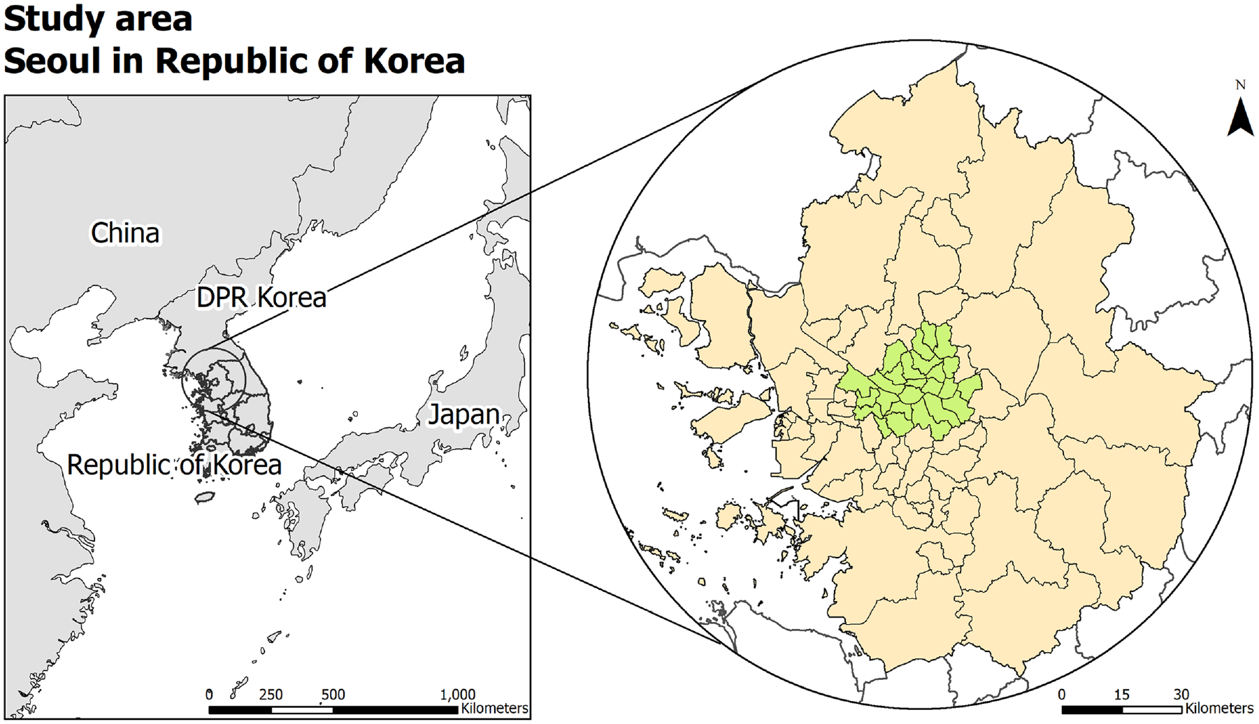
Study area.

To address the effects of the built environment on travel mode choice, 5Ds are employed in this analysis and collected based on the “dong” unit. Population density is measured as as density, employment density as accessibility to neighborhood services, road network density as design, mixed land use is calculated by an entropy index as diversity, distance to the nearest central business district (CBD) as accessibility to a destination, and the number of transit stops in the neighborhood as accessibility to transit. These are taken as built-environment variables that represent the 5Ds. Mixed land use is derived by an entropy index using residential, commercial, and industrial areas. Specifically, the entropy index is derived from $- \sum_{k} p_{i} \frac{\ln (p_{i})}{\ln (k)}$ , where $p_{i}$ is the proportion of the total land area of $i$ th land use category, and $k$ is the number of total land use categories. The larger the entropy value, the more complex the land use. Distance to the nearest CBD is obtained by measuring the distance to the nearest CBD location from the respondent’s home.

The descriptive statistics in Table 1 show that trip information, individual, and household characteristics differ across age groups but that the built-environment characteristics are not especially differentiated. Here, each age group is divided into young adults (25–40), middle-aged adults (41–64), and older adults (65+). According to the trip information of each age group, as age increases, travel time tends to be longer across all travel modes. In addition, travel time using the subway tends to be longer than for the other modes across all ages. Destination types are more distinct between groups. The older the respondent, the more travel to other places instead of work or school. When considering individual characteristics, older adults are less likely to have a driver’s license than young adults. That is, while about 80% of young and middle-aged adults have driver’s licenses, just about 50% of older adults have one. In relation to household characteristics, older adults’ households are less likely to own a car than other groups, and about 48% of their households are considered low-income. Unsurprisingly, the number of households having a child under 5 years old is higher in the young adult group. Lastly, of built-environment characteristics, distinct differences are not found among age groups. On average, people live in areas with densities of 24,000 people/km², 9,000 workers/km².

Table 1.

Descriptive Statistics of Variables

Variables	Description	Type	Young	Middle	Older
The number of samples			15,829	19,793	3,515
Trip information
Travel time (min)	Travel duration (minutes)	Drive alone	33.3	32.4	28.8
		Bus	40.3	37.8	37.7
		Subway	49.5	48.0	47.9
Destination type	Work, school, or others (%)	Work	86.61	83.31	37.41
		School	2.12	0.02	0.
		Others	11.26	16.68	62.59
Individual characteristics
Gender	Male or female (%)	Male	58.79	62.48	57.64
Driver license	None or licensed (%)	Licensed	85.28	83.86	49.19
Household characteristics
Car ownership	None or own (%)	Own	77.72	82.27	48.85
Monthly income	Monthly household income (%)	Low (under 2 million KRW)	6.2	8.43	48.25
		Middle (2–5 million KRW)	66.69	58.83	39.15
		High (over 5 million KRW)	27.1	32.74	12.6
Child in household	Child under 5 years old in household (%)	Yes	25.64	4.71	2.02
Built-environment characteristics
Population density	10,000 people/km²	Mean	2.41	2.4	2.33
		SD	1.16	1.15	1.17
Employment density	1,000 people/km²	Mean	10.06	9.55	8.8
		SD	11.32	10.64	9.1
Road network density	km/km²	Mean	6.64	6.65	6.62
		SD	2.87	2.84	2.83
Mixed land use	Entropy index using residential, commercial, and industrial areas	Mean	0.32	0.32	0.32
		SD	0.23	0.23	0.23
Distance to nearest CBD	Road network distance to the nearest CBD	Mean	7.63	7.69	7.65
		SD	3.63	3.54	3.51
Bus stops	The number of bus stops within 1 km	Mean	216.92	213.67	218.43
		SD	65.1	64.41	65.9
Subway stations	The number of subway stations within 1 km	Mean	6.7	6.56	6.56
		SD	4.04	3.89	3.82

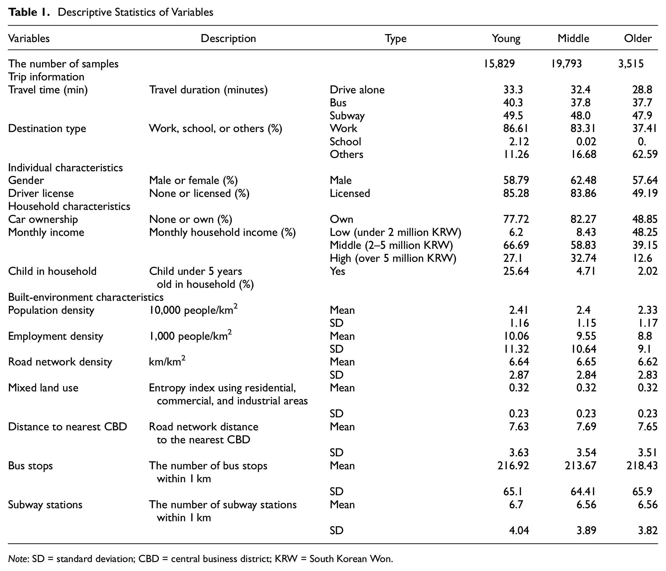
Note: SD = standard deviation; CBD = central business district; KRW = South Korean Won.

Figure 2 shows the spatial distribution of the built-environment variables applied in this analysis. The population is denser in the southwestern and northern areas than in the CBD of central Seoul (Figure 2a). These are densely populated residential areas. Employment density is highest in central Seoul and the southeastern area known as “Gangnam” (Figure 2b). Road density as design is also high in the southwestern and northern areas as well as the center of the city, which shows a similar pattern for population density except in the center (Figure 2c). Mixed land use calculated as the entropy index is high in the western areas (Figure 2d). When comparing this with the population density, mixed land use is lower in residential areas. The number of bus stops within 1 km is high along with population density (Figure 2e), whereas the number of subway stations within 1 km is high in central Seoul (Figure 2f). Figure 2g represents a distance to the nearest CBD. There are three CBDs in Seoul. The Seoul city hall is located in the geographical center of Seoul. Yeouido is a financial center and Gangnam is a commercial center in Seoul.

Figure 2.

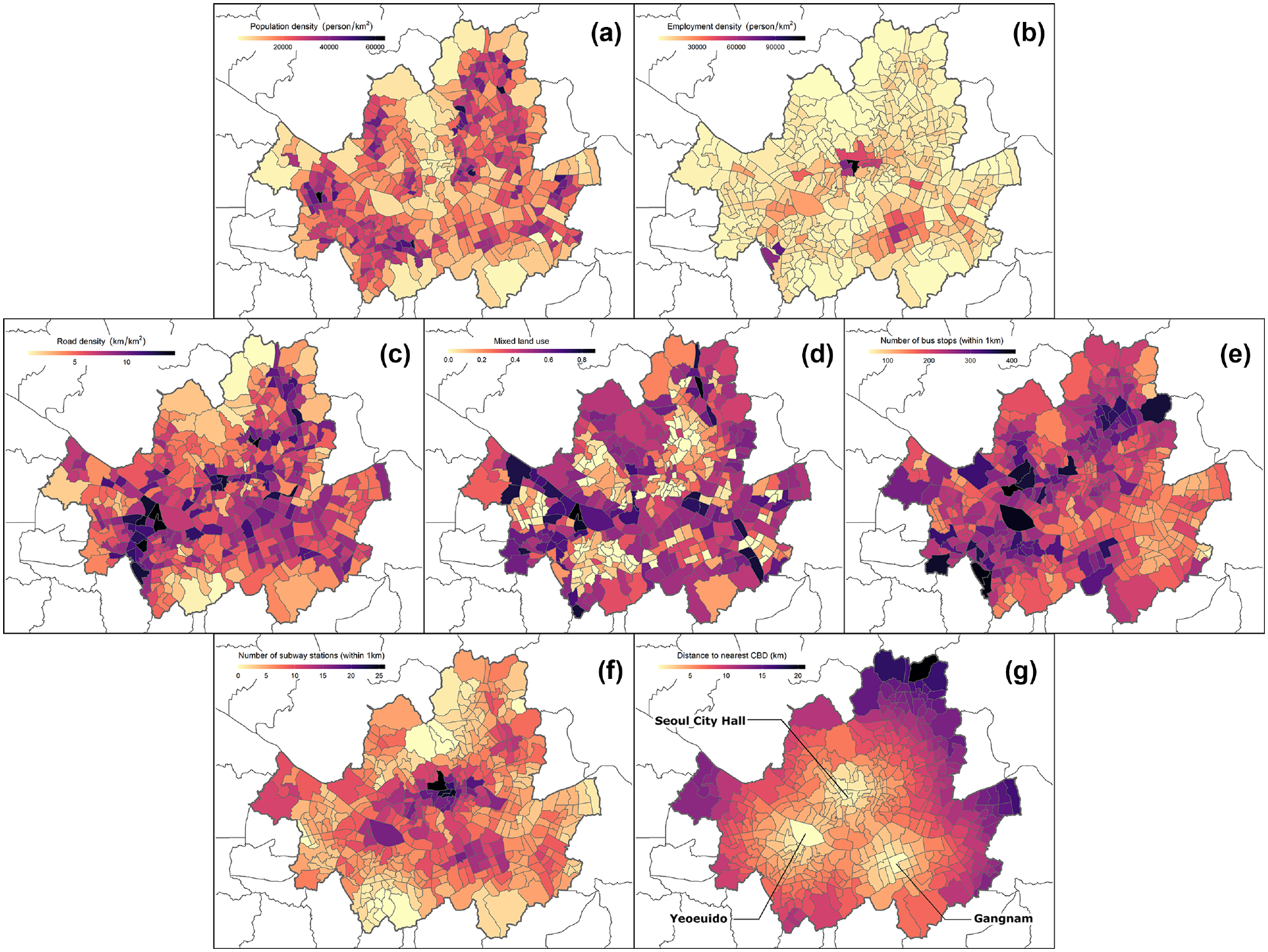
Maps of built-environment variables: (a) population density; (b) employment density; (c) road density; (d) mixed land use; (e) the number of bus stops; (f) the number of subway stations; and (g) distance to the nearest central business district (CBD).

Random Forest and Model Specification

RF is known as an ensemble method developed by Breiman ( 37 ) and has been employed in various classification exercises and regression modeling. RF is also known to be robust and insensitive to outliers, skewness of data distributions, and irrelevant variables ( 37 ). Prediction using RF results from a large collection of decision trees based on bootstrapping. In the method, each decision tree would not use all the explanatory variables, which lets the method overcome the weaknesses of a single decision tree, such as over-fitting and prediction errors resulting from biased samples and noisy data ( 38 ). Despite these benefits, it has been pointed out that interpreting the results of RF is challenging, which is similar to other machine learning methods ( 39 ). However, there have been advances in tools leading to better model interpretations. Thus, this study uses variable importance that indicates each variable’s influences and partial independent plots to capture the relationship between input variables and the probabilities of travel mode choices ( 33 ). These computations are conducted using randomForest and iml packages in R (32, 40).

There are key hyperparameters for determining prediction performance of the RF method: “mtry” (the number of splitting variables at each point); “ntree” (the total number of trees); and “depth” (the maximum tree depth). Although the result of RF is not sensitive to changes in hyperparameters, it would be expected that model performance would improve by calibrating them. To calibrate the hyperparameters, this study follows Cheng et al. ( 1 ) who tried to identify suitable values for mtry, ntree, and depth. Breiman ( 37 ) suggested that a suitable value for mtry was $lo g_{2} p$ . As the number of explanatory variables used in this study is 14 $(p)$ , the number of mtry would be about 4 according to the suggestion, whereas 2, 4, and 6 were compared to find the best value for mtry. Suitable numbers of depth and trees were searched from 50 to 500 by 50 and from 500 to 5000 by 500, respectively. To select the best calibrated hyperparameters, we consider error rates calculated by the models using the key hyperparameters with execution time. The difference here from Cheng et al. ( 1 ) is that this study considers mtry, ntree, depth, and execution time simultaneously. Taking all elements together, this study will identify optimal hyperparameters thereby reducing error rates.

In the RF method, the model should be trained using subdivided data at a ratio of 7:3. Here, 70% of the data are randomly selected and employed as training data, and the rest are used as testing data. The prediction performance of our model will be tested based on testing data.

The prediction performance of the model is assessed by the error rate calculated by an out-of-bag (OOB) sample. The error rate is described by errorOOB and calculated as follows:

errorOOB = (1 - \frac{1}{N} \sum_{i \in OOB} δ_{i}) \times 100 %

(1)

δ_{i} = {\begin{matrix} 1 & predict correctly \\ 0 & otherwise \end{matrix}

(2)

where errorOOB is the prediction error rate, and $δ_{i}$ denotes the correctness indicator variable. $N$ is the number of observations in the OOB sample. Using errorOOB, we identify optimal hyperparameters ( 1 ).

This study uses “mean decrease accuracy” to assess the importance of each variable across age groups.

VI (X_{j}) = \frac{1}{ntree} \sum_{f} (errorOO B_{f} - errorOO B_{fj})

(3)

where $VI (X_{j})$ is variable importance of $X_{j} (j = 1, \dots, M)$ that is the permuted variable, and M is the number of all predictors of the model. $errorOO B_{f}$ denotes the error of a single tree $f$ , and $errorOO B_{fj}$ is calculated by randomly permuting the value of $X_{j}$ . When $X_{j}$ is permutated in the OOB sample, the prediction accuracy decreases according to the prediction power of $X_{j}$ . The total difference between $errorOO B_{f}$ and $errorOO B_{fj}$ is divided by the number of trees and this is a variable importance of $X_{j}$ ( 41 ). In this study, the calculated variable importance is converted to percentages and rankings in each age group so that the importance of each variable can be compared.

Hyperparameters

An error rate and execution time are considered as criteria to determine the optimal value of the hyperparameters. Error rates lower than the ceiling of a minimum error rate are filtered, then the set of hyperparameters with the fastest execution time is selected. For instance, if error rates range from 28.3 to 32.5, candidates of error rate lower than 29 are selected. In the set of error rates lower than 29, that is, from 28.3 to 28.9, execution time determines hyperparameters.

First, for the young adult group, Figure 3a shows the distribution of error rates and cells satisfying the criteria. Based on the criteria, we settle on mtry = 4, ntree = 100, and depth = 1,500 in the RF method for the young adult group. Second, as can be seen in Figure 3b, based on the same criteria, mtry = 6, ntree = 100, and depth = 1,500 are selected for the middle-aged adult group. Although 4 and 6 mtry have both two cells satisfying the criteria, we choose 4 mtry based on the minimum value. Last, Figure 3c indicates the result of calibration for the older adult group. We settle on mtry = 2, ntree = 100, and depth = 2,000. As the error rates of the older adult group are lower than other groups, we could relax the criteria, but instead we decided to apply the same criteria to the selection.

Figure 3.

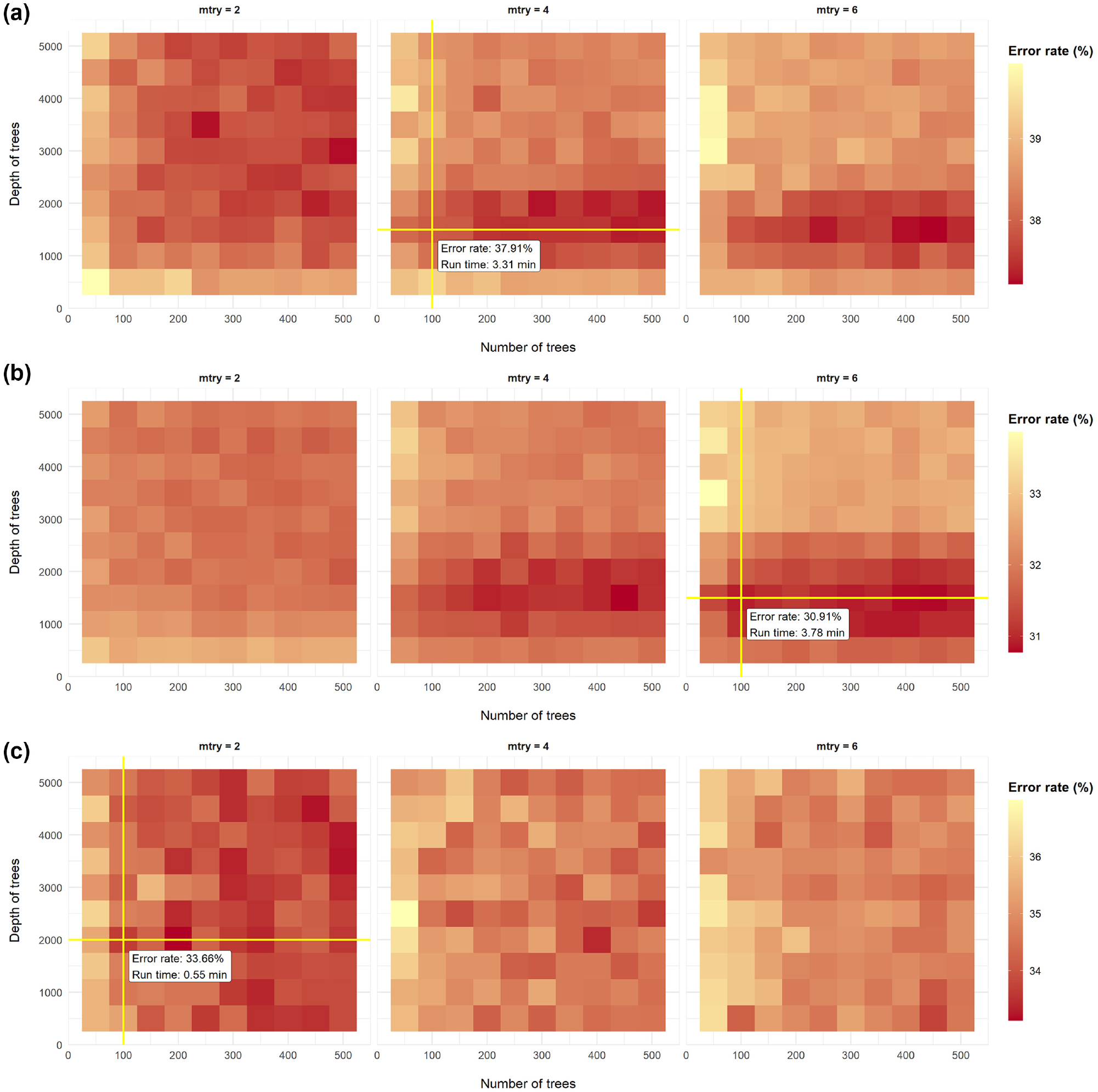
Hyperparameter optimization: (a) young adults; (b) middle-aged adults; and (c) older adults.

Analysis and Results

We executed our RF model using the selected hyperparameters to three motorized travel modes: drive alone, bus, and subway. Walking is also a considerable urban travel mode, but we only focus on the motorized mode in this study. The dataset is divided by the ratio of 7:3 as training data and testing data. In this section, the results of our RF model are reported based on the prediction results that use the testing data.

As can be seen in Table 2, the total number of trips that our dataset contains is 39,137 trips. In contrast with the United States which is developed to be more automobile-oriented, the share of driving alone is 41.74% in total trips and public transit (bus+subway) accounts for 58.26% of travel in Seoul. This trend differs across age groups. Older adults tend to use more public transit than other age groups, whereas middle-aged adults tend to use more automobiles than others. These differences may reflect the factors for choosing travel mode choice for each age group. In the same table, predicted rows show mode splits predicted by the RF model based on testing the dataset. While the share of driving alone is over-predicted for middle-aged adults, the overall predicted mode splits are similar to the mode splits of actual data.

Table 2.

Mode Splits of Actual and Predicted

Dataset	Age group	Drive alone	Bus	Subway	Subtotal
Actual	Young	5,684 (35.91%)	5,621 (35.51%)	4,524 (28.58%)	15,829 (100%)
	Middle-aged	9,860 (49.82%)	6,105 (30.84%)	3,828 (19.34%)	19,793 (100%)
	Older	791 (22.50%)	1,518 (43.19%)	1,206 (34.31%)	3,515 (100%)
	Total	16,335 (41.74%)	13,244 (33.84%)	9,558 (24.42%)	39,137 (100.00%)
Predicted	Young	2,254 (47.46%)	1,515 (31.90%)	980 (20.64%)	4,749 (100%)
	Middle-aged	3,671 (61.82%)	1,981 (33.36%)	286 (4.82%)	5,938 (100%)
	Older	312 (29.57%)	480 (45.50%)	263 (24.93%)	1,055 (100%)
	Total	6,237 (53.12%)	3,976 (33.86%)	1,529 (13.02%)	11,742 (100%)

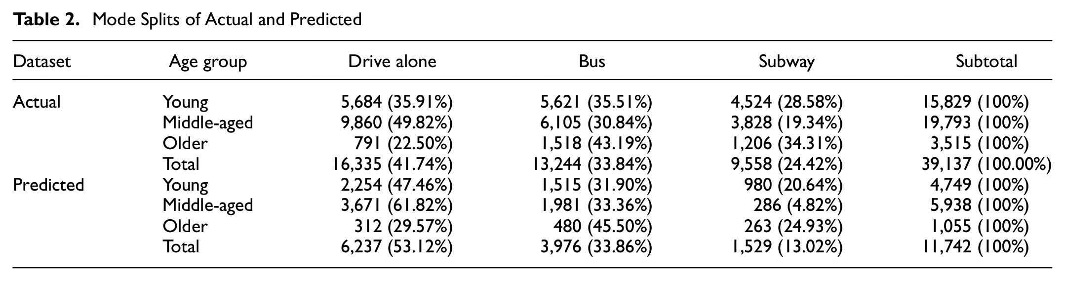
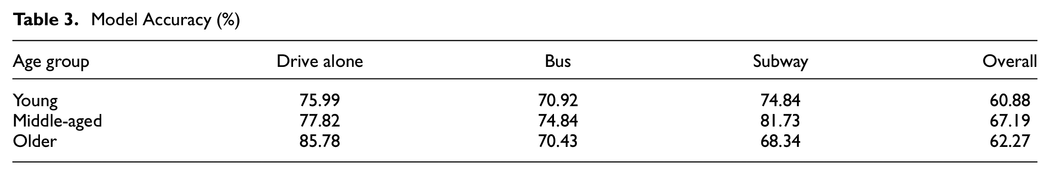
Table 3 represents the model accuracy of our RF model with each age group. The overall accuracies of all models are over 60% and each travel mode model accuracy is over 70% except for older adults’ choice for the subway (68.3%). While overall accuracy is slightly lower, each model’s accuracy is still considerable when comparing our accuracies with those of previous studies (e.g., 1, 34).

Table 3.

Model Accuracy (%)

Age group	Drive alone	Bus	Subway	Overall
Young	75.99	70.92	74.84	60.88
Middle-aged	77.82	74.84	81.73	67.19
Older	85.78	70.43	68.34	62.27

As can be seen in Figure 4, the percentage of importance of variables is visualized as a bar graph. Readers can refer to a table that contains values of importance and rank in the Supplemental Material. Overall, travel time, car ownership, and gender have a higher importance for choosing a travel mode across age groups.

Figure 4.

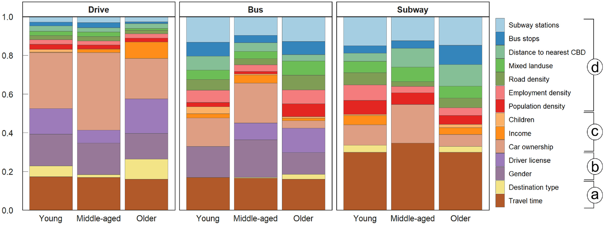
Importance by travel mode: (a) trip information, (b) individual characteristic, (c) household characteristic, and (d) built environment.

The importance of the built-environment variables is lowest in the selection of driving. Other characteristics, except for the built environment, better determine selection of driving. Across age groups, unsurprisingly, car ownership is the most crucial factor in the selection of driving compared with bus and subway. A noticeable trend is that the importance of the built-environment variables explains the choice of public transportation over that of driving. For instance, though there are some differences, the built-environment variables (portions of [d] in Figure 4) explain about 40% or more of the choice of bus or subway but less than 20% for the driving. Individual characteristics are not important in choosing subway compared with the others. While driver’s license and gender appear to be quite important variables in choosing driving and bus, they do not seem to affect people’s selection of the subway.

In contrast with driving, built-environment variables have much more influence on the bus and subway modes, accounting for more than half of the importance. Across all age groups, travel time is still a crucial factor in the choice of public transportation as well as driving, and its importance in the selection of the subway mode is more than 30%. Of the built-environment variables, the number of subway stations accounts for about 20% or less in the selection of bus and subway modes.

One of the key results is that individual characteristics do not seem to affect the selection of the subway mode for all age groups; gender and driver license are not related to the selection of the subway mode. In addition, relatively speaking, built-environment variables appear to have more importance on the selections of young and older adults for public transportation than that of middle-aged adults.

Table 4 presents how the variables are associated with people’s travel mode choice in relation to directions. We list the five most important variables for each travel mode choice. These associations are derived from partial dependence plots that show the marginal effect of a given variable on the predicted outcome of a machine learning model ( 33 ). A “positive sign” means that the probability of selecting a travel mode increases as a value of the variable increases. Conversely, a “negative sign” indicates that the probability of the selection decreases as a value of the variable increases. When the associate is not linear, we denote “non-linear” instead of simply positive or negative.

Table 4.

Direction of Associations

Age group	Travel mode	Variable	Importance	Direction of association	Category
Young	Drive alone	Car ownership (own)	28.95%	+	Household characteristic
		Travel time	17.27%	-	Trip information
		Gender (male)	16.38%	-	Individual characteristic
		Driver license (licensed)	13.27%	+	Individual characteristic
		Destination type	5.57%		Trip information
	Bus	Travel time	17.24%	Non-linear	Trip information
		Gender (male)	16.25%	+	Individual characteristic
		Car ownership (own)	14.84%	-	Household characteristic
		Subway stations	13.43%	-	Built environment
		Distance to CBD	7.36%	-	Built environment
	Subway	Travel time	33.49%	+	Trip information
		Subway stations	16.86%	+	Built environment
		Car ownership (own)	11.72%	-	Household characteristic
		Employment density	9.03%	+	Built environment
		Population density	8.07%	+	Built environment
Middle-aged	Drive alone	Car ownership (own)	40.26%	+	Household characteristic
		Travel time	16.96%	-	Trip information
		Gender (male)	16.29%	-	Individual characteristic
		Driver license (licensed)	6.77%	+	Individual characteristic
		Subway stations	3.11%	+	Built environment
	Bus	Car ownership (own)	20.62%	-	Household characteristic
		Gender (male)	19.42%	+	Individual characteristic
		Travel time	16.59%	+	Trip information
		Subway stations	9.60%	-	Built environment
		Driver license (licensed)	8.71%	-	Individual characteristic
	Subway	Travel time	49.89%	+	Trip information
		Car ownership (own)	28.85%	-	Household characteristic
		Subway stations	17.77%	+	Built environment
		Distance to CBD	13.89%	+	Built environment
		Mixed land use	10.76%	+	Built environment
Older adults	Drive alone	Car ownership (own)	21.14%	+	Household characteristic
		Driver license (licensed)	17.92%	+	Individual characteristic
		Travel time	16.21%	-	Trip information
		Gender (male)	13.36%	-	Individual characteristic
		Destination type	10.43%		Trip information
	Bus	Travel time	16.00%	Non-linear	Trip information
		Subway stations	12.79%	-	Built environment
		Driver license (licensed)	12.64%	-	Individual characteristic
		Gender (male)	11.32%	+	Individual characteristic
		Destination type	7.66%		Trip information
	Subway	Travel time	39.26%	+	Trip information
		Subway stations	19.27%	+	Built environment
		Distance to CBD	14.48%	Non-linear	Built environment
		Bus stops	13.20%	-	Built environment
		Mixed land use	8.19%	+	Built environment

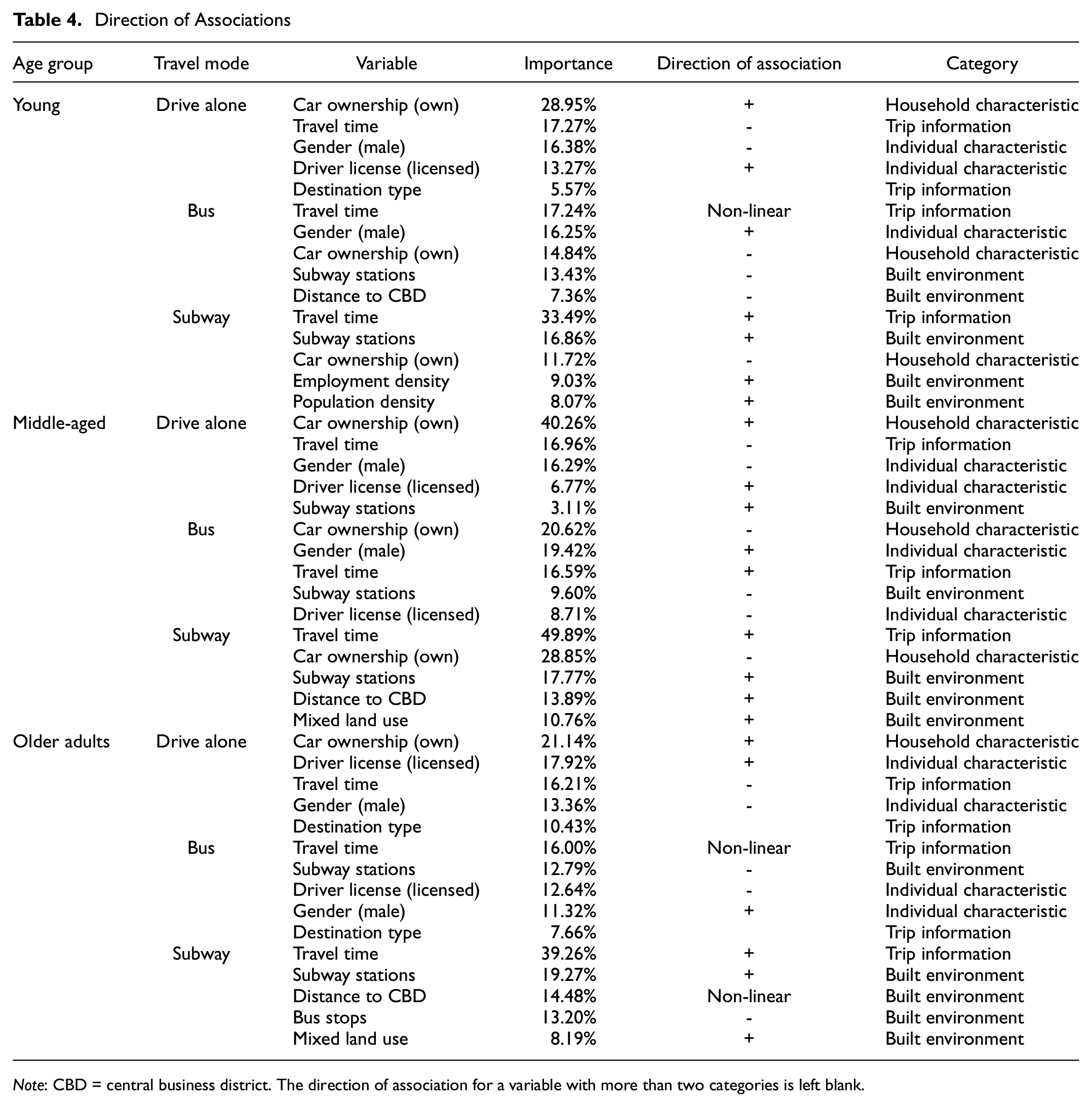
Note: CBD = central business district. The direction of association for a variable with more than two categories is left blank.

In the choice of driving for young adults, car ownership, travel time, gender, driver’s license, and destination type have about 81% importance. Here, car ownership and driver’s licenses have positive associations and travel time and gender have negative associations. On the other hand, travel time, gender, car ownership, subway stations, and distance to CBD determine about 69% for the bus selection. Unlike driving, gender has a positive association and other factors have a negative association. Built environment variables such as subway stations and distance to CBD are negatively related to the selection. Travel time has a non-linear relationship. The probability of bus selection goes up until a travel time of 25 min. If it takes more than 25 min, the probability is reduced (Figure 5a). For the subway, travel time, subway stations, car ownership, employment density, and population density determine about 80%. Except for car ownership, other variables have positive associations with the subway selection. In particular, the built-environment variables such as subway stations, employment density, and population density have a positive impact on the selection of the subway.

Figure 5.

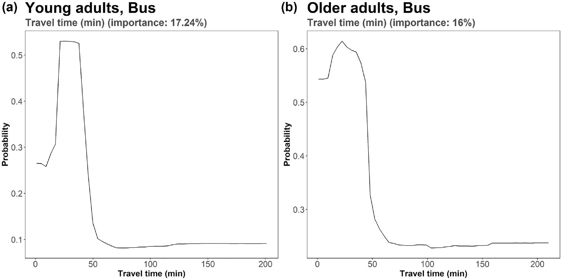
Non-linear relationships between travel time variable and bus selection: (a) young adults, and (b) older adults.

For middle-aged adults, the selection of driving is similar to that of young adults, and the number of subway stations has a positive effect on the selection. Bus selection is the opposite of driving selection. While the selection of the subway mode is similar to that of bus, travel time has almost a 50% importance to the selection, and built-environment variables such as subway stations, distance to CBD, and mixed land use appear to be the variables that have positive associations.

The choice of driving among older adults appears to have a similar tendency as other age groups. Females have a positive association with the bus selection, whereas subway stations, driver’s license, and destination type are negatively associated with the selection. In relation to travel time, it is found that the probability of bus selection increases until travel time reaches 25 min, but the probability decreases when it is 25 min, which is similar to the pattern with a travel time of young adults’ bus selection (Figure 5b). Except for bus stops, travel time, subway stations, and mixed land use are positively associated with the probability of subway selection. These five variables account for 94.4% of the importance to the selection.

In relation to the bus and subway selections, older adults respond differently to the distance to the nearest CBD compared with other age groups. The distance to the nearest CBD decreases the probability of bus selection for young and middle-aged adults, whereas the probability of older adults’ bus selection increases by 10 km then decreases (Figure 6, a–c). This pattern is reversed on the subway selection. While the distance to the nearest CBD increases the probability of subway selection for young and middle-aged adults, the probability of older adults’ subway selection decreases by 10 km then increases (Figure 6, d–f). The reason for this different pattern may reflect the older adults’ mobility challenges; for example, stairs and relatively long distances to subway platforms compared with bus stops may be a barrier to older adults with short travel distances.

Figure 6.

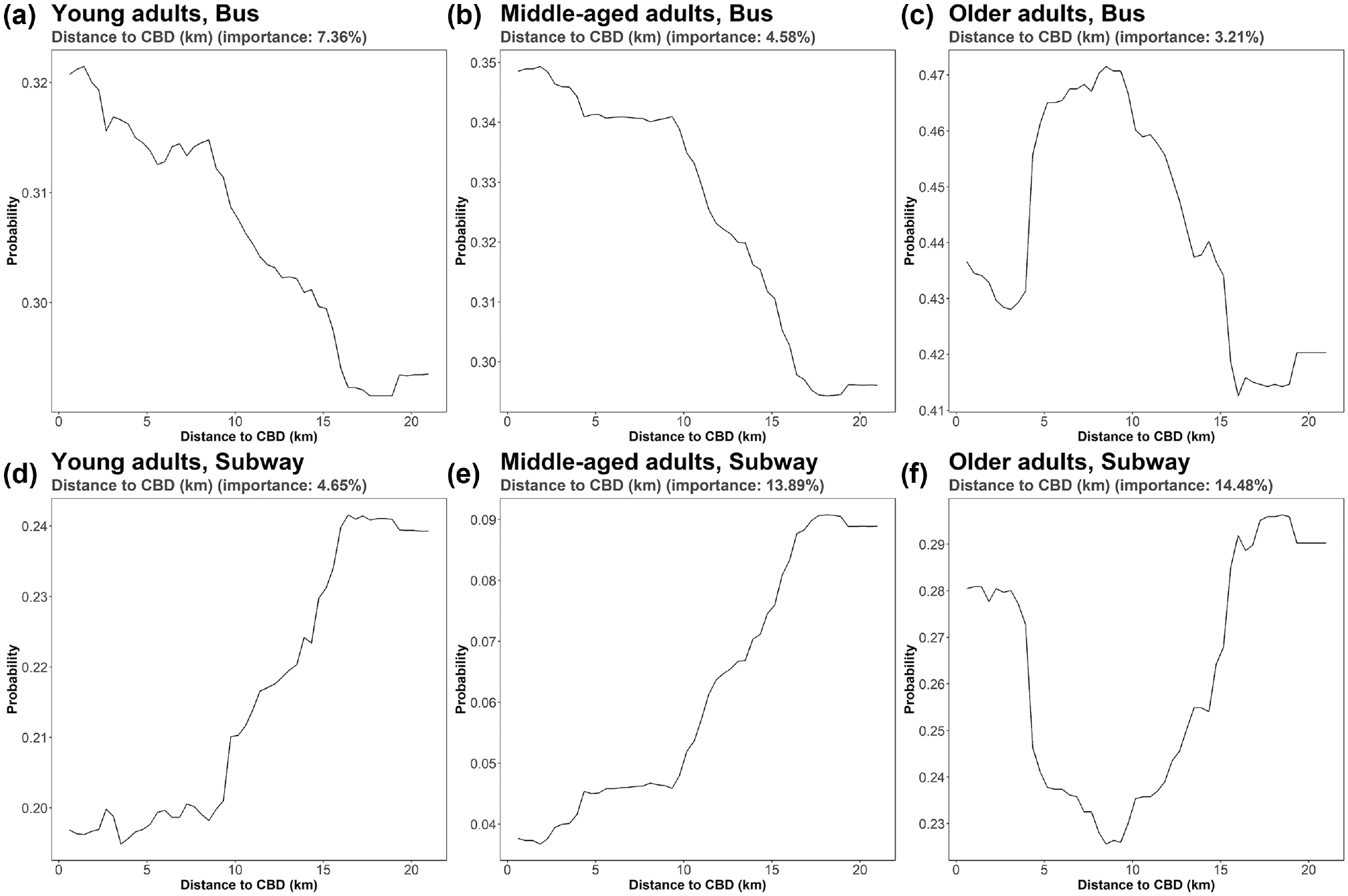
Comparison across age groups for bus and subway selection: (a) young adults, bus; (b) middle-aged adults, bus; (c) older adults, bus; (d) young adults, subway; (e) middle-aged adults, subway; and (f) older adults, subway.

The results are summarized as follows. Travel time reduces the probability of driving but decreases the chances of taking longer public transportation trips. If a passenger is a female, the probability of driving choice is lower than that of a male, but the probability of choosing a bus is higher than that of men ( 42 ). Built-environment variables do not significantly affect the probability of choosing driving, but they do increase the probability of choosing a subway ( 43 ). When comparing bus and subway, the number of subway stations reduces the probability of bus selection, and the greater the distance to the CBD, the more the probability of subway selection increases (7, 44).

Discussion and Conclusions

Using the rf, this paper examines the heterogeneous effects of attributes on travel mode choice across age groups in Seoul, South Korea, where public transportation systems are well established. Variable importance and partial dependence plots derived from the RF model help us discover what variables are important and how they are associated with the effect on travel mode choice. The analysis shows that attributes of the built environment have greater impact on the choice of public transportation than on driving. On the choice of public transportation among age groups, the built environment affects younger and older adults more than middle-aged adults.

Some results of this paper are, in general, consistent with findings of existing studies based on Western cities. For instance, females use the bus more frequently and do less driving than males ( 42 ). People who own a car in the household and have a driver’s license are more likely to use driving than public transportation (7, 45). In addition, there is a difference between choosing driving and the subway. Travel time has the opposite relationship on all age groups’ mode choice when comparing the subway selection with driving. For the subway selection, travel time is positively associated with the selection, whereas it has a negative association with driving ( 44 ). This may reflect the travel behavior of people in Seoul because travel using the subway might be perceived as comfortable and guarantee on-time arrival; the subay in the Seoul metropolitan area is sees as efficient while the traffic can often be heavy and congested. Longer travel times imply higher travel costs and result in cheaper modes being chosen over driving.

There are three significant features of our analysis. First, the built environment greatly influences public transportation choices but has little impact on driving. Although density has been emphasized as an important predictor in choosing public transportation in Western cities (30, 44), it does not have much importance in this study. One of the possible explanations might be related to Seoul being homogeneously dense. Second, the built environment, in particular, has a greater impact on the subway selection among older adults than other age groups. It is demonstrated that the built environment accounts for over 50% of the variation in subway selection for older adults although the set of attributes that influence the selection differs. This reveals that older adults are more sensitive to built-environment characteristics than other age groups (5, 15). Thus, it is crucial to change and develop the built environment to be more suitable to the mobility disabled to promote the usage of public transportation. Lastly, this analysis showed the opposite influences of some built-environment attributes on public transportation selection between older adults and other age groups and non-linear relationships. With these features, we conclude that RF has flexibility to capture the non-linearity and helps better understand the different effects of the built environment on travel mode choices across age groups. Thus, consequently, policy-makers may refer to these findings to promote the use of public transportation, considering different associations of the built environment with each age group.

This study has some limitations that should be addressed in future studies. First, we do not consider residential self-selection bias in travel mode choice because the spatial unit used in this study cannot fully capture it. Although Ewing et al. ( 46 ) suggested that the influence of the built environment on travel behavior might be stronger than the reverse direction, at least when analyzing cross-sectional data, this bias should be considered in future studies to avoid the overestimation of the effects of the built environment on travel mode choice. Second, this study only takes into account the travel mode choice of residents in Seoul city, assuming that their mode choice behavior differs from others living in Incheon city and Gyeonggi-do because of possible heterogeneity of travel behavior. Future studies should consider the heterogeneous travel mode choice behavior among residents living in Seoul metropolitan area. Lastly, although the trip chaining effect is considerable in travel mode choice analysis, we did not include the effect in our analysis because it is beyond our scope here. However, future research may consider capturing the trip chaining effect using machine learning methods.

Supplemental Material

sj-pdf-1-trr-10.1177_03611981211000750 – Supplemental material for Examining the Effects of the Built Environment on Travel Model Choice across Different Age Groups in Seoul using a Random Forest Method

Supplemental material, sj-pdf-1-trr-10.1177_03611981211000750 for Examining the Effects of the Built Environment on Travel Model Choice across Different Age Groups in Seoul using a Random Forest Method by Kyusik Kim, Kyusang Kwon and Mark W. Horner in Transportation Research Record

Footnotes

Author Contributions

The authors confirm contribution to the paper as follows: study conception and design: K. Kim and K. Kwon; data collection: K. Kim and K. Kwon; analysis and interpretation of results: K. Kim, K. Kwon, and M. W. Horner; draft manuscript preparation: K. Kim, K. Kwon, and M. W. Horner. All authors reviewed the results and approved the final version of the manuscript.

Declaration of Conflicting Interests

The author(s) declared no potential conflicts of interest with respect to the research, authorship, and/or publication of this article.

Funding

The author(s) received no financial support for the research, authorship, and/or publication of this article.

Data Accessibility Statement

The data that support the findings of this study were obtained from the 2016 Household Travel Survey at Korea Transport Database (). As these data are available to anyone publicly via this portal, the data sharing is not applicable to this article as no new data were created or analyzed in this study.

Supplemental Material

Supplemental material for this article is available online.

References

Cheng

Chen

De Vos

Lai

Witlox

Applying a Random Forest Method Approach to Model Travel Mode Choice Behavior. Travel Behaviour and Society, Vol. 14, 2019, pp. 1–10.

Cervero

Kockelman

Travel Demand and the 3Ds: Density, Diversity, and Design. Transportation Research Part D: Transport and Environment, Vol. 2, No. 3, 1997, pp. 199–219.

Ewing

Cervero

Travel and the Built Environment: A Synthesis. Transportation Research Record: Journal of the Transportation Research Board, 2001. 1780: 87–114.

Munshi

Built Environment and Mode Choice Relationship for Commute Travel in the City of Rajkot, India. Transportation Research Part D: Transport and Environment, Vol. 44, 2016, pp. 239–253.

Cao

X. (Jason)

Mokhtarian

P. L.

Handy

S. L.

Neighborhood Design and the Accessibility of the Elderly: An Empirical Analysis in Northern California. International Journal of Sustainable Transportation, Vol. 4, No. 6, 2010, pp. 347–371.

Cervero

Built Environments and Mode Choice: Toward a Normative Framework. Transportation Research Part D: Transport and Environment, Vol. 7, No. 4, 2002, pp. 265–284.

Ding

Wang

Liu

Zhang

Yang

Exploring the Influence of Built Environment on Travel Mode Choice Considering the Mediating Effects of Car Ownership and Travel Distance. Transportation Research Part A: Policy and Practice, Vol. 100, 2017, pp. 65–80.

Schwanen

Mokhtarian

P. L.

What Affects Commute Mode Choice: Neighborhood Physical Structure or Preferences toward Neighborhoods?

Journal of Transport Geography, Vol. 13, No. 1, 2005, pp. 83–99.

Zhang

The Role of Land Use in Travel Mode Choice: Evidence from Boston and Hong Kong. Journal of the American Planning Association, Vol. 70, No. 3, 2004, pp. 344–360.

10.

Rodríguez

D. A.

Joo

The Relationship between Non-Motorized Mode Choice and the Local Physical Environment. Transportation Research Part D: Transport and Environment, Vol. 9, No. 2, 2004, pp. 151–173.

11.

Rosenbloom

Sustainability and Automobility among the Elderly: An International Assessment. Transportation, Vol. 28, No. 4, 2001, pp. 375–408.

12.

Cao

X. (Jason)

. Heterogeneous Effects of Neighborhood Type on Commute Mode Choice: An Exploration of Residential Dissonance in the Twin Cities. Journal of Transport Geography, Vol. 48, 2015, pp. 188–196.

13.

Ding

Wang

Tang

Mishra

Liu

Joint Analysis of the Spatial Impacts of Built Environment on Car Ownership and Travel Mode Choice. Transportation Research Part D: Transport and Environment, Vol. 60, 2018, pp. 28–40.

14.

Xie

Chan

E. H. W.

Exploring Impacts of the Built Environment on Transit Travel: Distance, Time and Mode Choice, for Urban Villages in Shenzhen, China. Transportation Research Part E: Logistics and Transportation Review, Vol. 132, 2019, pp. 57–71.

15.

Cheng

Chen

Yang

Cao

De Vos

Witlox

Active Travel for Active Ageing in China: The Role of Built Environment. Journal of Transport Geography, Vol. 76, 2019, pp. 142–152.

16.

Cheng

De Vos

Shi

Yang

Chen

Witlox

Do Residential Location Effects on Travel Behavior Differ between the Elderly and Younger Adults?

Transportation Research Part D: Transport and Environment, Vol. 73, 2019, pp. 367–380.

17.

Feng

The Influence of Built Environment on Travel Behavior of the Elderly in Urban China. Transportation Research Part D: Transport and Environment, Vol. 52, 2017, pp. 619–633.

18.

Figueroa

M. J.

Nielsen

T. A. S.

Siren

Comparing Urban Form Correlations of the Travel Patterns of Older and Younger Adults. Transport Policy, Vol. 35, 2014, pp. 10–20.

19.

O’Hern

Oxley

Logan

Older Adults at Increased Risk as Pedestrians in Victoria, Australia: An Examination of Crash Characteristics and Injury Outcomes. Traffic Injury Prevention, Vol. 16, Supplement 2, 2015, pp. S161–S167.

20.

Siren

Hakamies-Blomqvist

Mobility and Well-Being in Old Age:

Topics in Geriatric Rehabilitation, Vol. 25, No. 1, 2009, pp. 3–11.

21.

U.S. Department of Transportation, Bureau of Transportation Statistics. National Transportation Statistics, Table 1-41. www.bts.gov as of October 2016. (https://www.bts.gov/content/commute-mode-share-2015)

22.

Sung

Lee

Jung

Identifying the Relationship between the Objectively Measured Built Environment and Walking Activity in the High-Density and Transit-Oriented City, Seoul, Korea. Environment and Planning B: Planning and Design, Vol. 41, No. 4, 2014, pp. 637–660.

23.

Kim

J.-K.

Ulfarsson

G. F.

Sohn

Transportation Deficiencies for Older Adults in Seoul, South Korea. Transportation Research Record: Journal of the Transportation Research Board, 2014. 2469: 76–88.

24.

Yan

Liu

Zhao

Using Machine Learning for Direct Demand Modeling of Ridesourcing Services in Chicago. Journal of Transport Geography, Vol. 83, 2020, p. 102661.

25.

Bantis

Haworth

Who You Are Is How You Travel: A Framework for Transportation Mode Detection Using Individual and Environmental Characteristics. Transportation Research Part C: Emerging Technologies, Vol. 80, 2017, pp. 286–309.

26.

Wang

Ross

C. L.

Machine Learning Travel Mode Choices: Comparing the Performance of an Extreme Gradient Boosting Model with a Multinomial Logit Model. Transportation Research Record: Journal of the Transportation Research Board, 2018. 2672: 35–45.

27.

Zhao

Yan

Van Hentenryck

Prediction and Behavioral Analysis of Travel Mode Choice: A Comparison of Machine Learning and Logit Models. Travel Behaviour and Society, Vol. 20, 2020, pp. 22–35.

28.

Hensher

D. A.

Ton

T. T.

A Comparison of the Predictive Potential of Artificial Neural Networks and Nested Logit Models for Commuter Mode Choice. Transportation Research E, Vol. 36, 2000, pp. 152–172.

29.

Xie

Parkany

Work Travel Mode Choice Modeling with Data Mining: Decision Trees and Neural Networks. Transportation Research Record: Journal of the Transportation Research Board, 2003. 1854: 50–61.

30.

Hagenauer

Helbich

A Comparative Study of Machine Learning Classifiers for Modeling Travel Mode Choice. Expert Systems with Applications, Vol. 78, 2017, pp. 273–282.

31.

Zhou

Wang

Bike-Sharing or Taxi? Modeling the Choices of Travel Mode in Chicago Using Machine Learning. Journal of Transport Geography, Vol. 79, 2019, p. 102479.

32.

Molnar

. Iml: An R Package for Interpretable Machine Learning. Journal of Open Source Software, Vol. 3, No. 26, 2018, p. 786. https://doi.org/10.21105/joss.00786.

33.

Friedman

J. H.

Greedy Function Approximation: A Gradient Boosting Machine. Annals of Statistics, 2001, pp. 1189–1232.

34.

Cheng

De Vos

Zhao

Yang

Witlox

Examining Non-Linear Built Environment Effects on Elderly’s Walking: A Random Forest Approach. Transportation Research Part D: Transport and Environment, Vol. 88, 2020, p. 102552.

35.

Ermagun

Rashidi

T. H.

Lari

Z. A.

Mode Choice for School Trips: Long-Term Planning and Impact of Modal Specification on Policy Assessments. Transportation Research Record: Journal of the Transportation Research Board, 2015. 2513: 97–105.

36.

Tribby

C. P.

Miller

H. J.

Brown

B. B.

Werner

C. M.

Smith

K. R.

Analyzing Walking Route Choice through Built Environments Using Random Forests and Discrete Choice Techniques. Environment and Planning B: Urban Analytics and City Science, Vol. 44, No. 6, 2017, pp. 1145–1167.

37.

Breiman

Random Forests. Machine Learning, Vol. 45, No. 1, 2001, pp. 5–32.

38.

Rodriguez-Galiano

V. F.

Ghimire

Rogan

Chica-Olmo

Rigol-Sanchez

J. P.

An Assessment of the Effectiveness of a Random Forest Classifier for Land-Cover Classification. ISPRS Journal of Photogrammetry and Remote Sensing, Vol. 67, 2012, pp. 93–104.

39.

Zhao

Yan

Van Hentenryck

Modeling Stated Preference for Mobility-on-Demand Transit: A Comparison of Machine Learning and Logit Models. arXiv:1811.01315 [cs, stat], 2018.

40.

Liaw

Wiener

Classiﬁcation and Regression by RandomForest. R News, Vol. 2, No. 3, 2002, pp. 18–22.

41.

Kawakubo

Yoshida

Rapid Feature Selection Based on Random Forests for High-Dimensional Data. Information Processing Society of Japan, 2012, p. 7.

42.

Scheiner

Holz-Rau

Gendered Travel Mode Choice: A Focus on Car Deficient Households. Journal of Transport Geography, Vol. 24, 2012, pp. 250–261.

43.

Xie

Chan

How Does the Built Environment Influence Public Transit Choice in Urban Villages in China?

Sustainability, Vol. 11, No. 1, 2018, p. 148.

44.

Chen

Gong

Paaswell

Role of the Built Environment on Mode Choice Decisions: Additional Evidence on the Impact of Density. Transportation, Vol. 35, No. 3, 2008, pp. 285–299.

45.

Schwanen

Dieleman

F. M.

Dijst

Travel Behaviour in Dutch Monocentric and Policentric Urban Systems. Journal of Transport Geography, Vol. 9, No. 3, 2001, pp. 173–186.

46.

Ewing

Hamidi

Grace

J. B.

Compact Development and VMT—Environmental Determinism, Self-Selection, or Some of Both?

Environment and Planning B: Planning and Design, Vol. 43, No. 4, 2016, pp. 737–755.

Supplementary Material

Please find the following supplemental material available below.

For Open Access articles published under a Creative Commons License, all supplemental material carries the same license as the article it is associated with.

For non-Open Access articles published, all supplemental material carries a non-exclusive license, and permission requests for re-use of supplemental material or any part of supplemental material shall be sent directly to the copyright owner as specified in the copyright notice associated with the article.

0.00 MB

0.11 MB