
Abstract
Relatively recent increased computational power and extensive traffic data availability have provided a unique opportunity to re-investigate drivers’ car-following (CF) behavior. Classic CF models assume drivers’ behavior is only influenced by their preceding vehicle. Recent studies have indicated that considering surrounding vehicles’ information (e.g., multiple preceding vehicles) could affect CF models’ performance. An in-depth investigation of surrounding vehicles’ contribution to CF modeling performance has not been reported in the literature. This study uses a deep-learning model with long short-term memory (LSTM) to investigate to what extent considering surrounding vehicles could improve CF models’ performance. This investigation helps to select the right inputs for traffic flow modeling. Five CF models are compared in this study (i.e., classic, multi-anticipative, adjacent-lanes, following-vehicle, and all-surrounding-vehicles CF models). Performance of the CF models is compared in relation to accuracy, stability, and smoothness of traffic flow. The CF models are trained, validated, and tested by a large publicly available dataset. The average mean square errors (MSEs) for the classic, multi-anticipative, adjacent-lanes, following-vehicle, and all-surrounding-vehicles CF models are 1.58 × 10⁻³, 1.54 × 10⁻³, 1.56 × 10⁻³, 1.61 × 10⁻³, and 1.73 × 10⁻³, respectively. However, the results show insignificant performance differences between the classic CF model and multi-anticipative model or adjacent-lanes model in relation to accuracy, stability, or smoothness. The following-vehicle CF model shows similar performance to the multi-anticipative model. The all-surrounding-vehicles CF model has underperformed all the other models.
Highly automated vehicles (HAV) will share roads with conventional vehicles as early as the end of this decade ( 1 ). Mixed traffic flow of conventional vehicles and HAVs could influence traffic flow by increasing vehicle miles traveled (VMT), change in headway, and/or change in drivers’ behavior ( 2 ). Assessing mixed traffic flow behavior requires understanding human and HAVs’ driving behavior. HAVs’ behavior follows specific rules and algorithms known to the developers ( 3 ). However, human driving behavior is complex and hardly understood.
Human driving behavior is typically categorized into two distinct groups: (1) car-following (CF) behavior, and (2) lane-changing behavior. CF studies the longitudinal behavior of vehicles when one vehicle follows another ( 4 ). CF behavior has been studied since the 1950s ( 5 ). Most CF models assume drivers’ CF behavior is solely influenced by their preceding vehicle ( 5 – 7 ). However, recent studies claim that surrounding vehicles (e.g., vehicles in the adjacent lanes) may influence human CF behavior ( 8 – 15 ).
The goal of this study is to determine whether considering the surrounding vehicles’ information could improve CF models’ performance, and if the performance improvement is statistically significant. To achieve this goal, the following framework is proposed:
Developing five car-following models based on a deep-learning algorithm;
Fairly comparing the CF models’ performance at the local level and global level.
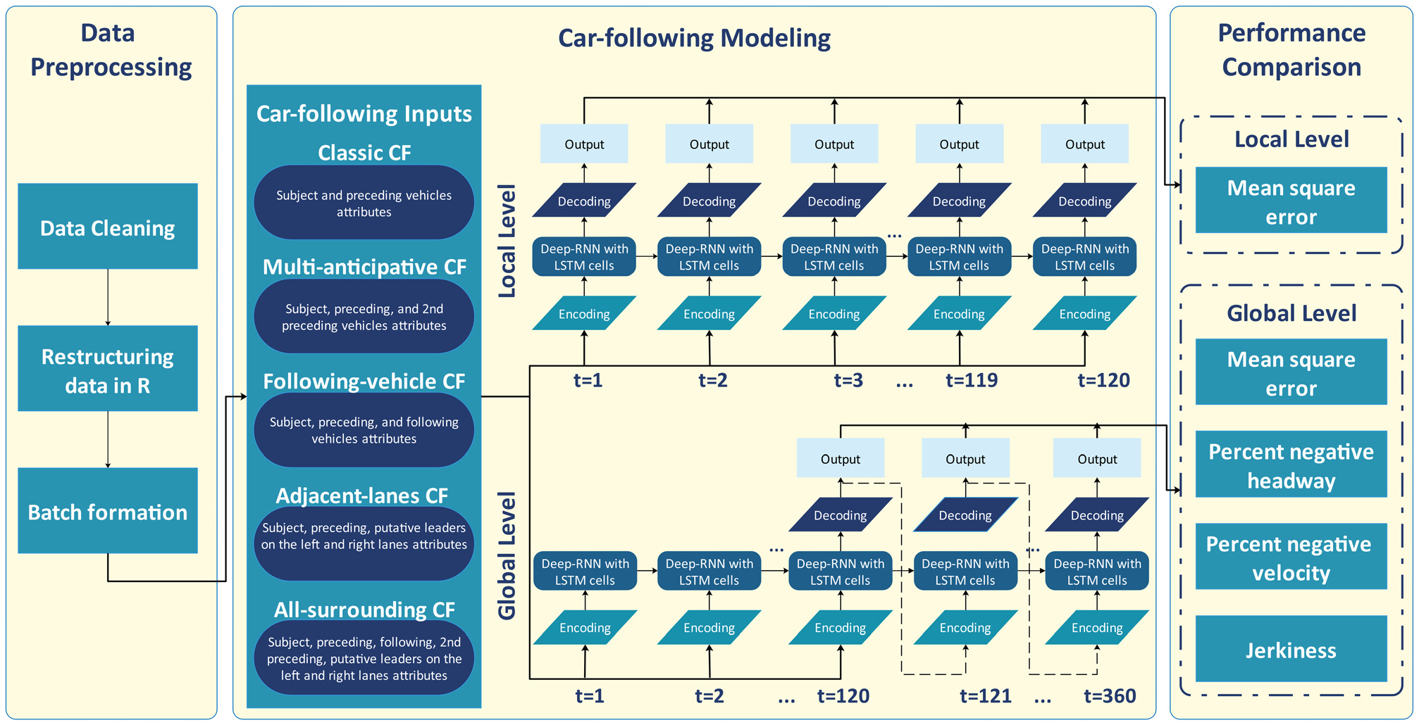
In this study, the surrounding vehicles are defined according to Figure 1, including preceding, following, the second preceding vehicle, and putative leaders on the left and right lanes. This study develops five CF models using a deep-recurrent neural network (deep-RNN) with long short-term memory (LSTM). All the models use identical deep-RNN architecture with identical configurations. The key difference between the CF models is their inputs. The CF models’ names and inputs are defined as:
Classic CF model: Considers the subject vehicle and the preceding vehicle’s attributes;
Multi-anticipative CF model: Considers the subject vehicle, the preceding, and the second preceding vehicles’ attributes;
Following-vehicle CF model: Considers the subject vehicle, the preceding, and the following vehicles’ attributes;
Adjacent-lanes CF model: Considers the subject vehicle, the preceding vehicle, and the attributes of putative leaders on the left and right lanes;
All-surrounding-vehicles CF model: Considers all the surrounding vehicles’ attributes (i.e., preceding, following, the second preceding vehicle, and putative leaders on the left and right lanes).
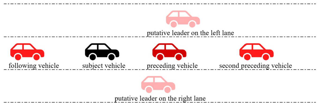
Car-following schematic
This study proposes two new CF models, based on the following vehicle and all surrounding vehicles. Multi-anticipative CF models suggested adding information from vehicles on the same lane could improve CF models’ accuracy and stability ( 8 , 10 , 16 ). Integrating information from both preceding and following vehicles could create forward and backward connections between vehicles, improving CF models’ stability and accuracy. This is the main idea behind the following-vehicle CF model. Moreover, a CF model integrating both multi-anticipative and adjacent-lanes models might explain human driving behavior more accurately. So, the all-surrounding-vehicles CF model might outperform other CF models.
This study proposes a fair comparison framework that compares five CF models and minimizes the risk of bias and randomness in the results. The framework compares the CF models’ performance at the local level (i.e., single-step single-vehicle predictions) and the global level (i.e., multi-step multi-vehicle predictions). To manage bias, assumption-free modeling (i.e., data-driven modeling) is used instead of parametric approaches (e.g., full velocity difference model). The authors also have included several measures (e.g., identical initial seeds, cross-validation, and dynamic stop-condition) to minimize randomness in the comparison. The framework is explained in the Method section.
This study makes several contributions, including modeling CF behavior by a novel deep-learning approach, developing two new CF models, investigating the surrounding vehicles’ contributions by real traffic data, and proposing a framework to minimize bias and randomness in the comparison. This is the first study of its kind using real-world traffic data to investigate the surrounding vehicles’ impacts. Similar studies used numerical simulations, with no actual traffic data involved in testing their models, except Papathanasopoulou and Antoniou, who used ten trajectories ( 12 ). These numerical simulations may not represent human driving behavior. This study utilizes more than 2,000 trajectories for a realistic and robust comparison. This study developed a novel deep-learning model with LSTM cells to boost CF models’ ability to regenerate naturalistic driving behavior. The authors are not aware of any previous study using deep-learning to model surrounding vehicles’ affects on CF behavior. The study proposed two new CF models, which are explained in the Method section in detail.
Literature Review
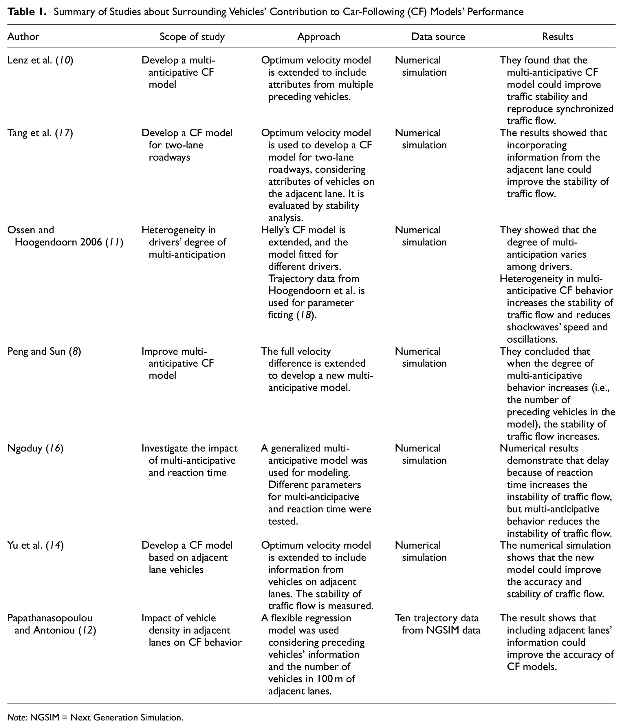
Most CF studies assume drivers’ behavior is only affected by their preceding vehicles ( 5 – 7 ). Recent studies argue that other surrounding vehicles could influence drivers’ CF behavior ( 8 , 10 – 13 , 15 ). Lenz suggested considering information from a series of preceding vehicles to predict a driver’s CF behavior, known as the multi-anticipative CF model ( 10 ). Other multi-anticipative models have been proposed by incorporating well-known CF models (e.g., optimum velocity difference and full velocity difference) to consider information from more than one preceding vehicle ( 9 , 16 ). These studies found that multi-anticipative CF models could improve the accuracy or stability of traffic flow ( 8 , 10 , 16 ). Details of these studies are reported in Table 1.
Summary of Studies about Surrounding Vehicles’ Contribution to Car-Following (CF) Models’ Performance
Note: NGSIM = Next Generation Simulation.
Some studies have explored the impact of vehicles in the adjacent lanes on drivers’ CF behavior ( 12 – 15 , 17 ). Ponnu and Coifman have studied drivers’ speed choice and headway choice in highway lanes ( 13 , 15 ). They reported that drivers in uncongested lanes reduce their speeds when the adjacent lanes are congested. Papathanasopoulou and Antoniou have proposed a CF model based on vehicle density in the adjacent lanes ( 12 ). The results showed that considering vehicle density in the adjacent lanes could increase CF models’ accuracy ( 12 ).
Although some studies have evaluated the potential impacts of the surrounding vehicles on CF models’ performance, these studies are not validated with real-world traffic data ( 8 , 10 , 14 , 16 , 17 ). The models are evaluated by numerical simulations, as is shown in Table 1. However, numerical simulations may not accurately represent human driving behaviors. Besides, all the studies used parametric CF models. The parametric models have been proposed based on some assumptions about human driving behavior, but these assumptions may not be valid for the surrounding vehicles. For example, drivers maintain desired velocity or headway from their preceding vehicles, but drivers may not be willing to maintain the desired velocity or headway from the vehicles in the adjacent lanes. Modeling surrounding vehicles’ effects based on parametric models could lead to significant bias and miscalculations. The previous studies also have not reported which combination of surrounding vehicles’ information could provide the best performance for CF modeling.
In recent years, deep-learning models have shown high performance in regenerating human CF behavior ( 19 – 28 ). Wang et al. proposed a deep-learning based CF model, using a neural network with gated recurrent unit (GRU) cells ( 23 ). A GRU cell is a simplified type of LSTM, without output gate, and with relatively lower performance than LSTM ( 29 ). The model was trained with the Next Generation Simulation (NGSIM) dataset and compared with the feedforward neural network (FNN) and intelligent driver model (IDM). The deep-learning model illustrated higher performance than both FNN and IDM models ( 23 ). Wang et al. studied the impact of long-term memory on CF models’ performance ( 25 ). They developed a deep-learning model with GRU cells. The model was trained with 3 s trajectories (i.e., short memory) and 10 s trajectories (i.e., long memory), using the NGSIM dataset. The results indicated that the model with long memory outperformed the short-memory model. They concluded that using long-term memory has a significant impact on CF models’ performance ( 25 ). Zhu et al. proposed a CF model based on deep deterministic policy gradient (DDPG) ( 21 ). DDPG is a well-known deep reinforcement learning technique that utilizes policies and rewards to train a model instead of memory and weights, which are used for deep neural networks. The model was trained by 2,000 trajectories from the Shanghai Naturalistic Driving dataset and compared with IDM, FNN, recurrent neural network (RNN), and Loess regression model. DDPG outperformed the other models with 23.5 root mean square percentage space error, in comparison with RNN, IDM, Loess, and FNN with 24, 24.5, 31, and 40 root mean square percentage space error, respectively. Tang et al. proposed a CF model based on GRU and Markov theory to improve CF models’ accuracy in low-speed traffic flow ( 27 ). The model was trained by the NGSIM dataset and compared with FNN, GRU, and full velocity difference (FVD) models. A traffic simulation showed that the new model has higher accuracy and stability than the other models.
LSTM is a type of neural network cell with short-term (i.e., hidden state) and long-term memory (i.e., cell state), which has illustrated strong performance in predicting time series ( 30 ). More information about LSTM’s structure is provided in the Background section. Huang et al. proposed a deep-learning CF model with LSTM ( 24 ). The model could regenerate the asymmetric characteristics of CF behavior (e.g., hysteresis and intensity difference), and it had a higher accuracy than FVD and RNN models ( 24 ). Vasebi et al. compared a parametric model (i.e., IDM), two machine learning models (i.e., FNN and RNN), and a deep-learning-with-LSTM model, using the NGSIM dataset ( 22 ). The result demonstrated that the deep-learning model has a significantly lower percentage headway error (i.e., 3.2 × 10⁻⁷) than IDM, FNN, and RNN with 5.8 × 10⁻², 8.9 × 10⁻³, and 5.0 × 10⁻³, respectively ( 22 ). Zhang et al. integrated a CF model with a lane-changing model in a deep-learning model with LSTM ( 28 ). The deep-learning model with one hidden layer could predict both CF and lane-changing behaviors with high accuracy ( 28 ).
This study sheds light on these issues by an in-depth and fair comparison between CF models that consider different surrounding vehicles’ attributes. This study utilizes around 300,000 observations from the NGSIM dataset to validate its results ( 31 ). This study develops a comparison framework based on deep-RNN with LSTM (i.e., a data-driven model). Unlike parametric models, a data-driven approach finds patterns using raw traffic data without any pre-assumption, resulting in an assumption-free model and comparison ( 19 ). This data-driven approach minimizes bias in the conclusion ( 32 ). Additionally, this study compares five CF models, providing a comprehensive conclusion about which surrounding vehicle’s information, and to what extent this information, improves CF models’ performance.
Background
This section provides background information about deep-learning, RNN, LSTM, and the other techniques used in this study.
The deep-learning method is used for this study because multiple studies have shown its outstanding performance in predicting human CF behavior ( 19 – 28 ). Deep-learning models with LSTM cells have three advantages which make them suitable for CF models:
Drivers do not make decisions in a moment: Vehicles’ trajectories are time series. Current status depends on both the current situation (e.g., current velocity difference and headway) and previous states (e.g., accelerations). Deep-learning with LSTM has a short-term memory (i.e., hidden state) that could remember the last few states. It uses this information to make an accurate prediction ( 33 , 34 ).
Drivers have long-term memory: Deep-learning with LSTM has a long-term memory (i.e., cell state), which learns long-term patterns in data ( 30 , 35 ). The deep-learning model could use this capability to recall long-term driving patterns ( 25 ). Conventional data-driven models are not able to learn long-term patterns (e.g., driving style and memory). This unique advantage aids the deep-learning models to achieve a higher accuracy level than traditional CF models ( 22 , 25 , 28 ).
A deep-learning model has high learning capability: A deep-learning model consists of multiple neural network layers. Each layer learns simple patterns. The output of one layer is fed to the next layer. This cascading learning process boosts the deep-learning models’ ability to learn complex driving behaviors ( 19 , 22 , 32 , 35 ).
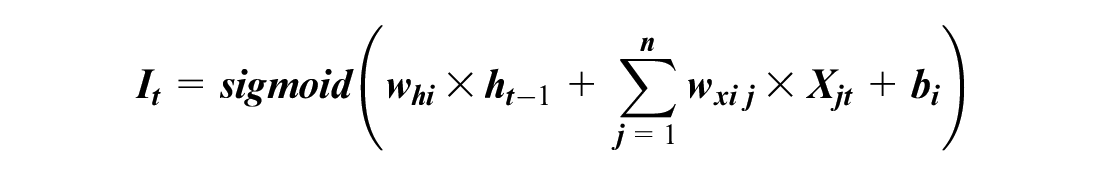
The deep-learning model which is employed in this study is a deep-RNN. The RNN is an advanced version of an FNN that receives inputs at the current time step (Xt) and a hidden state (ht-1) to produce the output (ht) ( 34 ). The hidden state carries the cell’s output from the previous time step to the next time step. This hidden state aids the model to find patterns in a sequence of data ( 33 , 34 ). Therefore, RNN effectively predicts time-series data and could learn human driving behavior, including drivers’ reaction delay ( 19 ). An RNN cell operates as:

where
n is the number of inputs.
In the first hidden layer,
An RNN model attempts to minimize the difference between the predicted output (
A deep-RNN consists of several RNN layers with LSTM cells. Several RNN layers create a cascading training process in which outputs of one layer are used as inputs for the next layer. Each layer learns a small portion of an intricate pattern, and all layers together could learn intricate patterns in data. The structure of a deep-RNN with three hidden layers is shown in Figure 2. The figure shows that the hidden state passes from one time period to another, and the output of one layer is used as an input for the next layer.
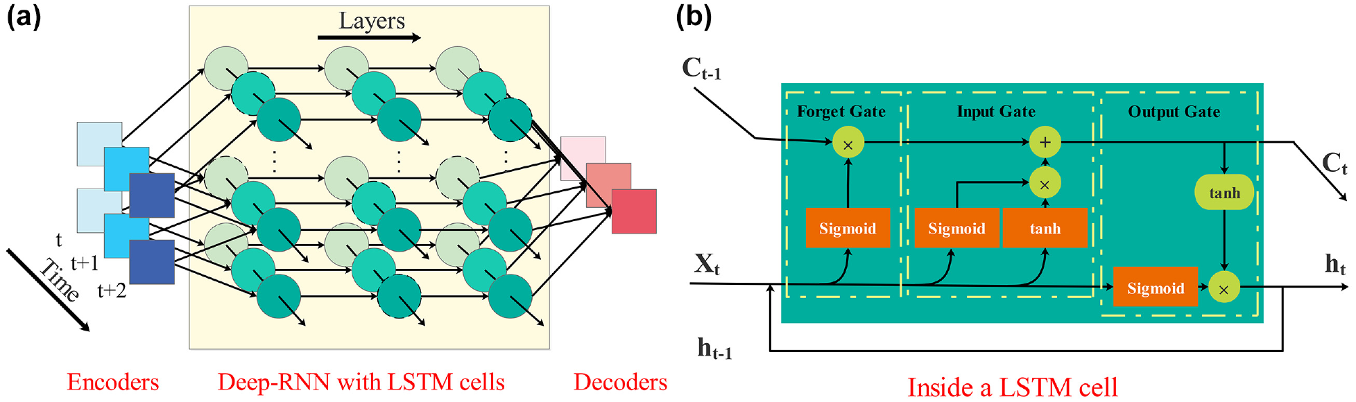
(a) Deep recurrent neural network (deep-RNN) and (b) long short-term memory (LSTM) cell in this study.
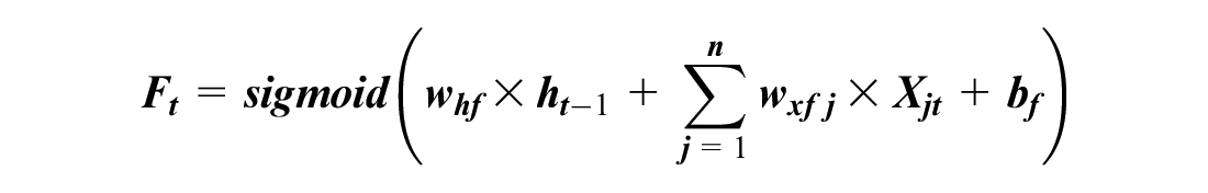
A normal RNN cell has one internal memory (i.e., hidden state), but an LSTM cell has two internal memories (i.e., hidden and cell states). The hidden state changes every time step, and it generates short-term memory. The cell state creates a long-term memory, and it could learn driving habits and long-term patterns. The cell state (Ct–1) is gradually updated based on the input values (Xjt) and the hidden state (ht–1) by a mechanism inside an LSTM cell (Figure 2). Ct–1 is updated through the forget gate and input gate, and Ct–1 is applied to the output (ht) by the output gate. Each gate has its own neural cell with weights, biases, and activation functions. The gates control information flow by adding (⊕) or multiplying (⊗) values. The operations in an LSTM cell are:
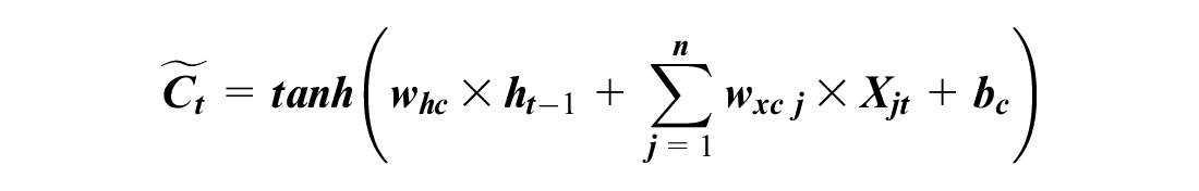

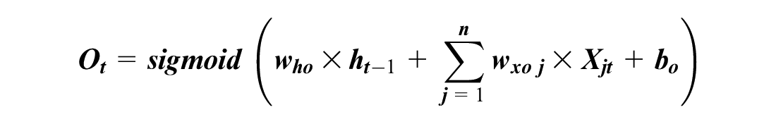

where
and
These weights and biases are optimized through the training process by gradient descent.
This study utilizes a drop-out technique to prevent overfitting. The drop-out randomly deactivates some cells in each training epoch, and it equally distributes weights and biases among all cells. Further information about the drop-out technique is available from Srivastava et al. ( 37 ).
Method
This study develops a framework to compare five CF models fairly. The framework includes three modules: 1) data preprocessing, 2) CF modeling, and 3) performance comparison, which are shown in Figure 3.
Car-following (CF) models’ comparison framework.
Data Preprocessing
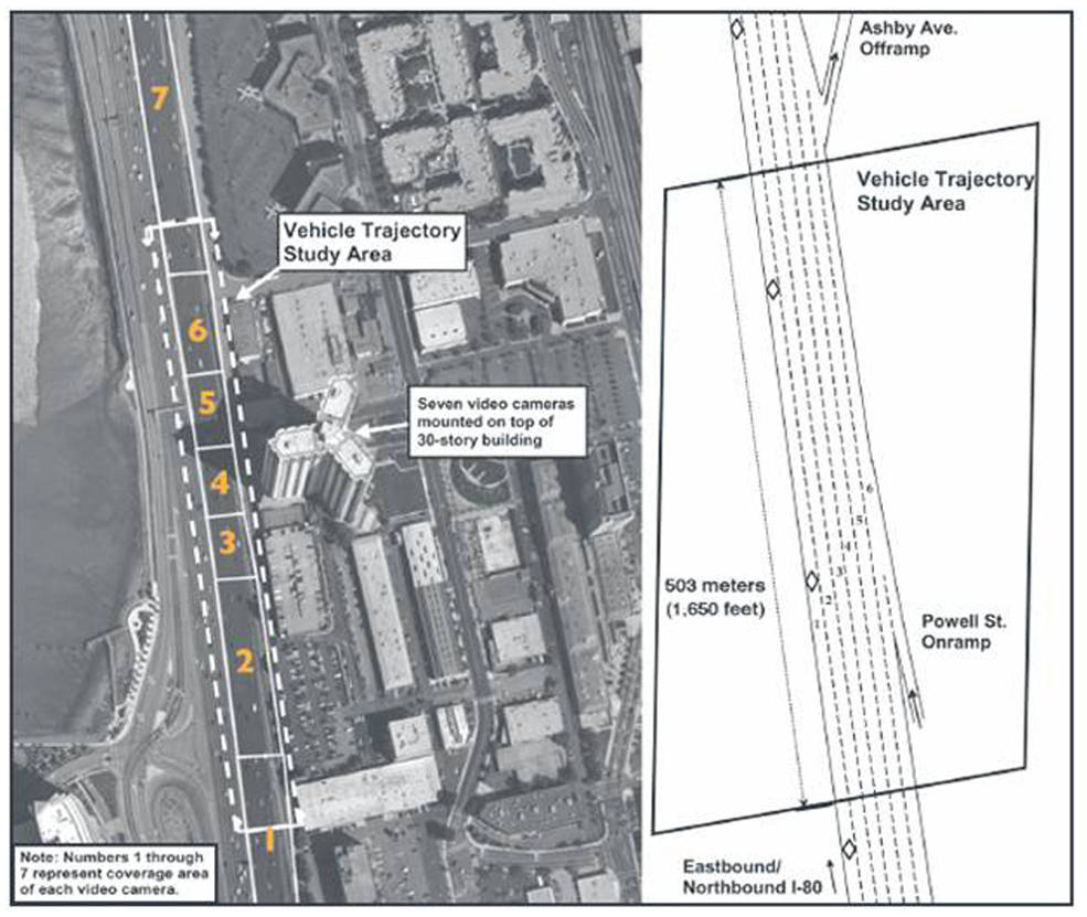
This study uses the NGSIM dataset from the Interstate 80 freeway (I-80) in Emeryville, California ( 31 ). The Federal Highway Administration (FHWA) gathered this dataset by seven video cameras mounted on top of a building next to the freeway (Figure 3). FHWA extracted the traffic data from the videos using an image processing software, and it discretized the data ( 31 ). The freeway has four regular freeway lanes, a high-occupancy vehicle lane (HOV), and a ramp at this location (Figure 4). More information about this dataset is available from FHWA ( 31 ).
Top view of I-80 study area. The drawing on the right shows the highway with its lane numbers (1: high-occupancy vehicle (HOV) lane; 2: left-most lane; 3–4: middle lanes; and 5: right-most lane) ( 31 ).
This study uses reconstructed NGSIM data in which outliers were removed, trajectories were smoothened by a low-pass filter, and traffic flow was reconstructed and validated ( 38 ). More information about the reconstructed NGSIM is available from Montanino and Vincenzo ( 38 ). The data was cleaned by removing missing data. The authors deployed an R code to generate required surrounding vehicles’ attributes (i.e., feature engineering) for each subject vehicle (e.g., velocity difference between the subject and the second preceding vehicle).
Drivers in different lanes may react differently to their surrounding vehicles. As an example, drivers on the HOV lane may pay less attention to vehicles on the other lanes because the HOV lane is isolated from the rest of the highway. Therefore, the five CF models are compared on each lane independently. The NGSIM data has been divided into groups of vehicles on HOV, left-most lane, middle lanes, and right-most lane, shown in Figure 3 with lane numbers 1, 2, 3–4, and 5, respectively.
The dataset is divided into batches with 120 observations. The batch size is selected according to Zhou et al. to provide enough long-term memory for the deep-learning model ( 26 ). The dataset is then divided into training, validation, and testing datasets, which are 70%, 10%, and 20% of the whole dataset, respectively (Figure 5). The whole dataset is divided by a set of random seeds, which were identical among all the five CF models. So, all the models receive identical training, validation, and testing datasets.
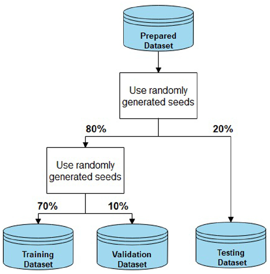
Dividing the Next Generation Simulation (NGSIM) dataset for training, validation, and testing.
Car-Following (CF) Modeling
All five CF models are developed based on an identical deep-learning network. The key difference between the models is their inputs. Inputs of the CF models are shown in Table 2. It should be noted that the vehicles’ velocity difference and headway refer to the subject vehicle’s speed difference and distance from those vehicles (e.g., the preceding vehicle’s headway is the headway between the subject and preceding vehicles).
The Car-Following (CF) Models’ Inputs
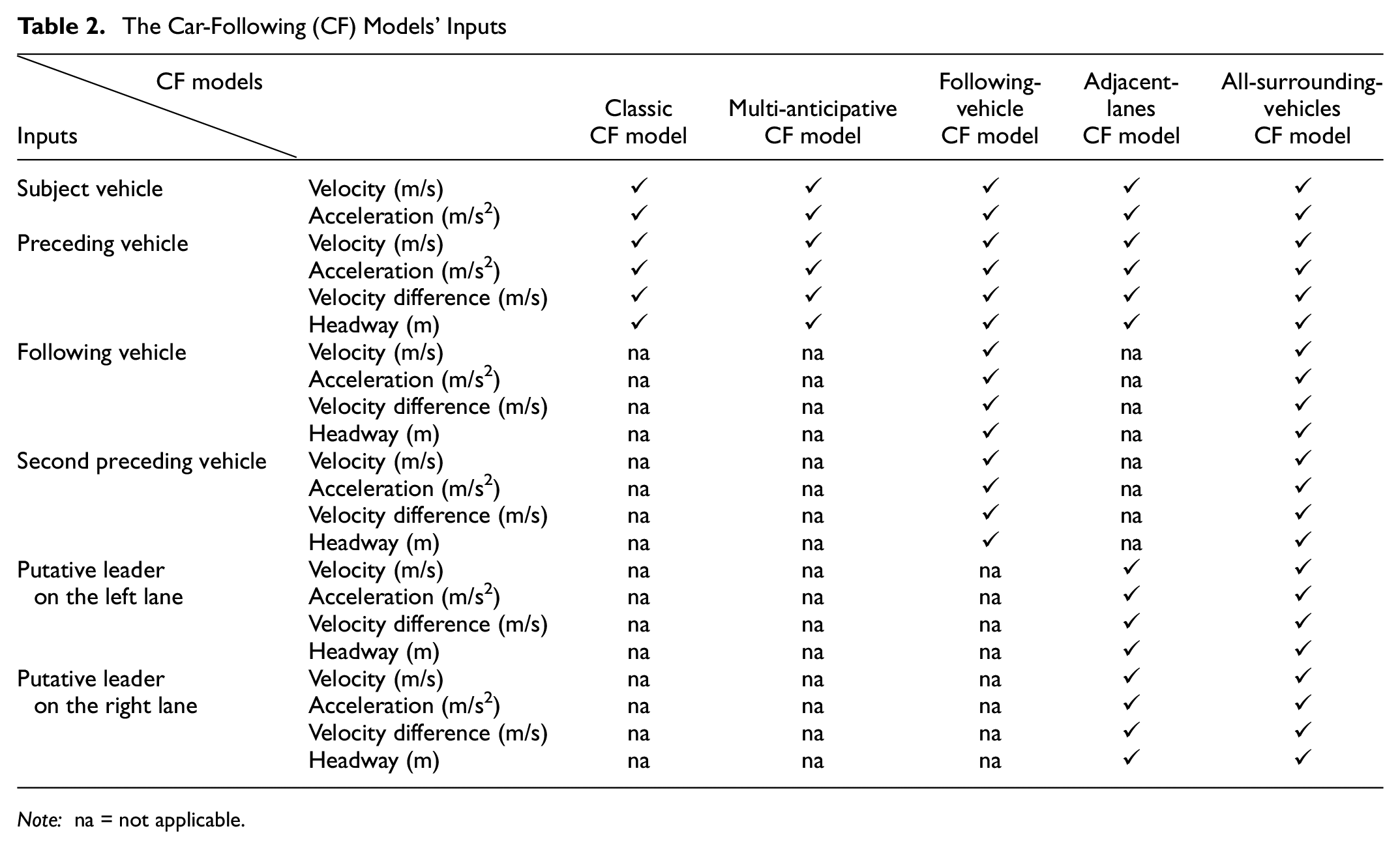
Note: na = not applicable.
In this study, the classic CF model is defined as a deep-learning-based model receiving the preceding and the subject vehicles’ attributes. The classic CF model does not refer to parametric models (e.g., IDM). As is shown in Figure 4, the input data are encoded and fed to the deep-learning model. The input data is encoded by the min-max function. The deep-learning model is developed based on a deep-RNN network with LSTM cells, as it is described in the Background section. The deep-RNN model has three hidden layers with 40 LSTM cells at each layer. The number of hidden layers and cells has been chosen after fine-tunings to achieve optimum performance. Sensitivity analysis on the number of hidden layers and cells has been performed in this manuscript, and further information is available from the authors.
Figure 2 shows the exact structure of the deep-RNN and LSTM cells which are used in this study. It should be noted that this study used deep-RNN with fully connected layers and 40 cells in each hidden layer, but these details are not shown in the figure because of lack of space. Xt is the CF models’ inputs in time t, fed to the model after encoding. The output of deep-RNN is the subject vehicle’s acceleration in the next time step (i.e., t + 1), which is decoded by the min-max function and sent for performance analysis. The deep-learning model is developed by the authors and coded in Python 3.6 by TensorFlow 1.15. TensorFlow is a library which is developed by Google DeepMind for coding deep-learning models ( 39 ).
The training procedure is shown in Figure 6. The deep-RNN CF models are trained by the training dataset. Through this training process, the deep-RNN uses gradient descent to reduce mean square error (MSE) between the predicted accelerations and actual accelerations. At the end of each training epoch, the validation dataset is used to provide an unbiased evaluation of modeling fitting. The training continues if the validation’s MSE improves. Otherwise, the training process is stopped, and the model’s performance is measured by the testing dataset. This stop-training strategy judges the quality of learning based on an unseen validation dataset. Validation-based stop-condition performs better than “training with a fixed number of epochs” and reduces the risk of overfitting or underfitting. The LSTM cells are warmed up and trained through the training process. Then, they are applied for the testing trajectories.
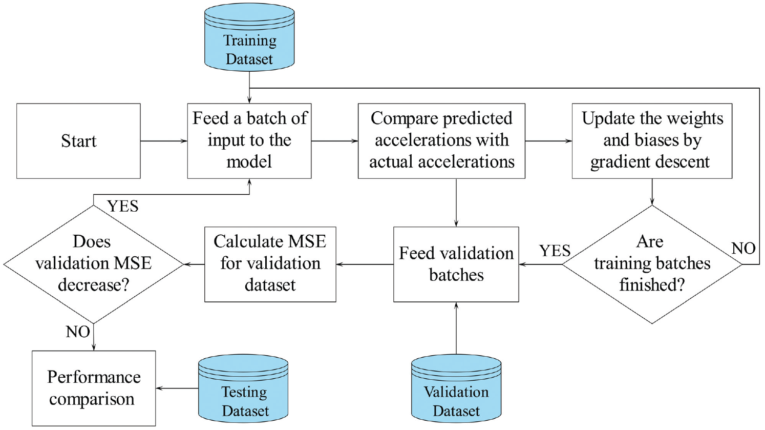
The deep recurring neural network (deep-RNN) training procedure.
Performance Comparison
The five CF models’ performances are compared at the local level and the global level. At the local level, the CF models receive a batch of inputs in the current time step (t), and they predict the subject vehicle’s acceleration in the next time step (t + 1). The models’ performances are compared based on average MSE. The procedure to compute the performance measure is shown in Figure 7.
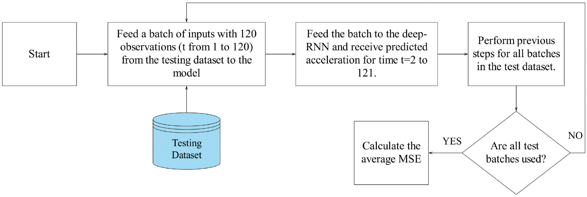
The procedure to calculate the car-following (CF) models’ performance measure at the local level.
Average MSE is calculated as:

where
The global level is a multi-step multi-vehicle assessment in which the CF models could regenerate a realistic traffic flow for a platoon of vehicles (i.e., a group of vehicles are following one another). For the global level assessment, traffic flow is simulated in Python and TensorFlow when a platoon of six vehicles travels for 240 time steps (i.e., 24 s). The procedure for this traffic simulation is shown in Figure 8.
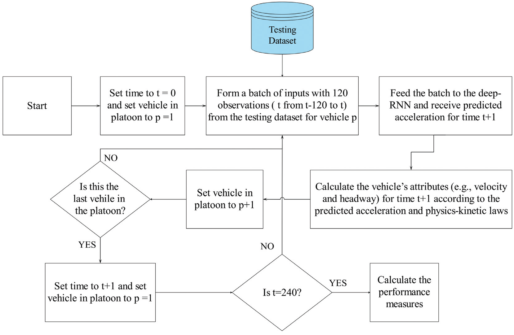
The procedure to calculate the car-following (CF) models’ performance measures at the global level.
The goal of global level assessment is to evaluate the CF models’ ability to regenerate accurate, stable, and smooth traffic flow. The accuracy is measured by MSE between the simulated accelerations and the actual accelerations. The stability is measured by percent negative headway and percent negative velocity. The smoothness is measured by the level of jerkiness ( 19 ). The level of jerkiness calculates the percentage of change in the jerk sign. In physics, “jerk” is defined as the derivative of acceleration. When jerk value changes from positive to negative, or vice versa, its sign changes, illustrating a jerky driving behavior. The percentage of change in jerk sign demonstrates the level of smoothness or jerkiness of a trajectory.
Fair Comparison Strategies
The goal of this study is to provide a fair comparison across the five CF models. Therefore, a fair comparison framework developed considers:
Cross-validation: All the CF models are trained with 80% of data (i.e., training and validation) and tested by 20% of data. Each model is trained and tested for 30 rounds. The models’ average performance is used for the comparison. The 30 full rounds provide six rounds of full cross-validation (i.e., 20% × 30 = 600%).
Identical training and testing data: Training and testing datasets are assigned by random seeds. The seeds are identical across all the models at each round of the comparison. So, all the models receive identical datasets for their training, validation, and testing.
Overfitting and underfitting: Deep-RNN is prone to overfitting and underfitting. Deep-RNN’s training should be stopped at the right moment to avoid overfitting or underfitting. A validation-based stop-condition is used to prevent overfitting or underfitting. This stop-condition is explained in the Car-Following (CF) Modeling section and Figure 6. Moreover, the drop-out technique is employed to reduce the risk of overfitting.
Further information about modeling, coding, and the hyperparameters is available from the authors on request.
Analysis of variance (ANOVA) and Z-test investigate the significance of the performance difference between CF models. ANOVA test is applied to verify if there is a significant performance difference between the models ( 40 ). If the ANOVA test is significant, Z-test is applied to find which pair of CF models have significant performance differences.
In this study, multiple ANOVA and Z-tests are performed, which could cause multiple comparisons problem. This problem arises when many statistical tests are performed, and a random pattern might be identified as statistically significant (i.e., false-positive) ( 41 ). Several approaches have been proposed for multiple testing correction. This study uses the Benjamini–Yekutieli procedure ( 42 ). In the Benjamini–Yekutieli procedure:
The tests’p-values are sorted in ascending order.
The procedure finds the largest k, which:

where

The procedure rejects the null hypothesis for the tests ranked i = 1, …, k.
More information about this procedure is available from Benjamini and Yekutieli ( 42 ).
Results
The deep-RNN code was run 1,200 times for comparison at the local and global levels (i.e., 2 levels × 5 CF models × 4 lanes × 30 runs = 1,200) and 1,800 times for sensitivity analysis (i.e., 2 levels × 5 CF models × 6 configurations × 30 runs = 1,800). Each run took between 5 and 40 s on Intel i5-6400 with 8Gb RAM.
Performance Comparison at the Local Level
Figure 9 shows how the deep-RNN model performs in predicting human CF behavior. This figure shows three predicted acceleration trajectories. These trajectories have an average MSE of 1.60 × 10⁻³, which is the average MSE for all CF models on all lanes in this study. This figure illustrates that deep-RNN can predict CF behavior with high accuracy in single-step predictions. Most of the predicted accelerations fit the actual accelerations, except at the peaks, where the predicted trajectories are smoother than the actual trajectories.
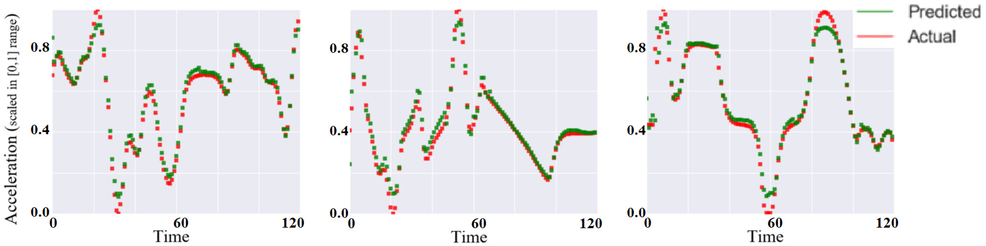
Average performance of the deep recurring neural network (deep-RNN) at the local level (three acceleration trajectories with an average performance of mean square error (MSE) = 1.60 × 10⁻³).
Average MSE of all CF models explored are reported in the top part of Table 3 for all highway lanes. The models with the lowest MSE values are shown in bold. ANOVA test indicates that the null hypothesis is rejected on all the lanes, except on the middle lane. For the lanes with significant ANOVA values, Z-test is conducted. The right-most column of Table 3 shows the significance of the performance difference between the CF models. As an example, “3–5” means the performance of the third CF model (following-vehicle CF model) is significantly different from the fifth CF model (all-surrounding-vehicles CF model).
The Car-Following (CF) Models’ Mean Square Error (MSE) at the Local Level and their MSE, % Negative Headway, % Negative Speed, and Jerkiness at the Global Level for the Highway’s Lanes, and Significance of their Performance Difference
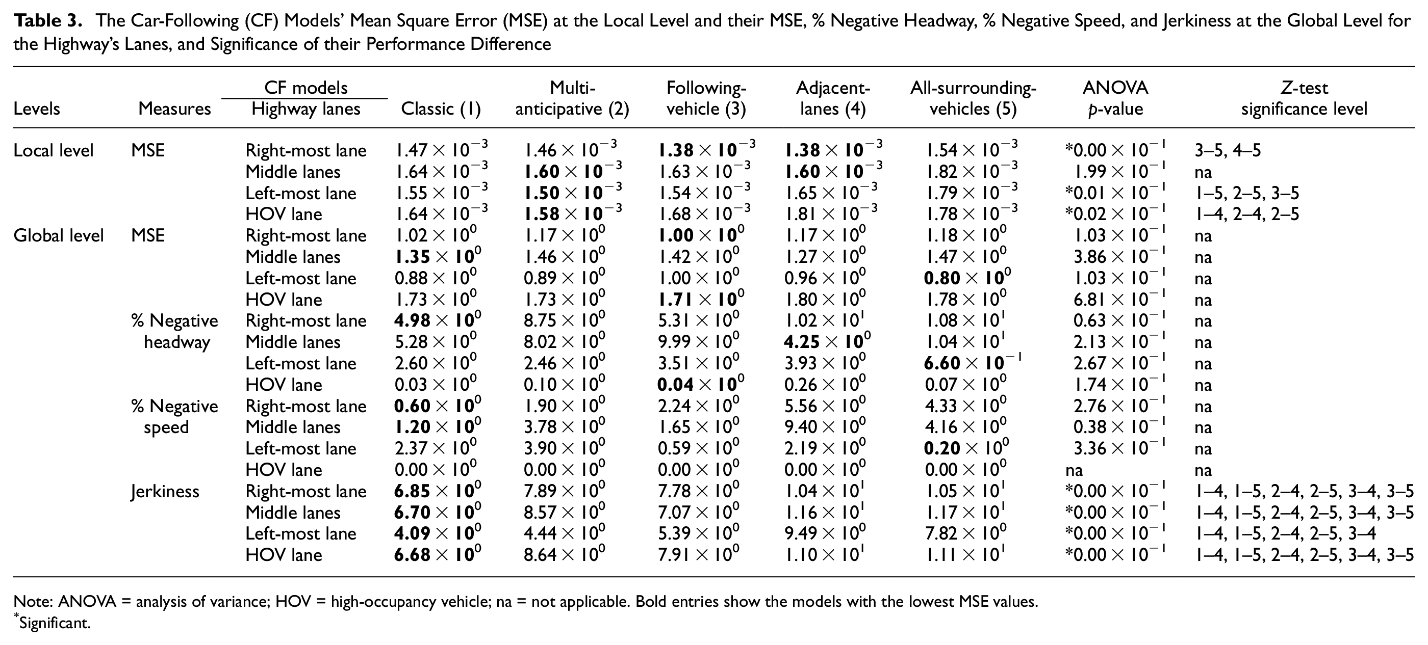
Note: ANOVA = analysis of variance; HOV = high-occupancy vehicle; na = not applicable. Bold entries show the models with the lowest MSE values.
Significant.
This result indicates that the all-surrounding-vehicles CF model performs significantly worse than the other CF models on all lanes, except on the middle lane. On the middle lane, the all-surrounding-vehicles CF model has the worst performance with no significant difference from the others. Adjacent-lanes CF model is the best-performing model on the right-most lane and the middle lane. However, its accuracy decreases on the left-most lane and the HOV lane. There is not enough evidence to prove a significant performance difference between following-vehicle, multi-anticipative, and classic CF models.
Performance Comparison at the Global Level
Figure 10 shows the performance of the deep-learning model in predicting human CF behavior at the global level. This figure shows results for traffic simulation for a platoon of six vehicles. The figure compares the vehicles’ predicted acceleration trajectories with their actual acceleration trajectories. The deep-RNN closely follows the first vehicle’s actual acceleration on the platoon (i.e., vehicle #1) for the first few predictions. After a few steps, the deep-RNN is not able to follow the actual accelerations, but it maintains a stable traffic condition and reacts to the main stimuli in the traffic flow. The following simulated vehicles respond to the main stimuli of the simulated preceding vehicle, not the actual preceding vehicle. So, the following simulated vehicles’ accelerations are not like their actual acceleration trajectories. Instead, their acceleration trajectories follow their simulated preceding vehicles with delay. This behavior illustrates a stable traffic simulation, which is shown at the velocity-time and location-time diagrams.
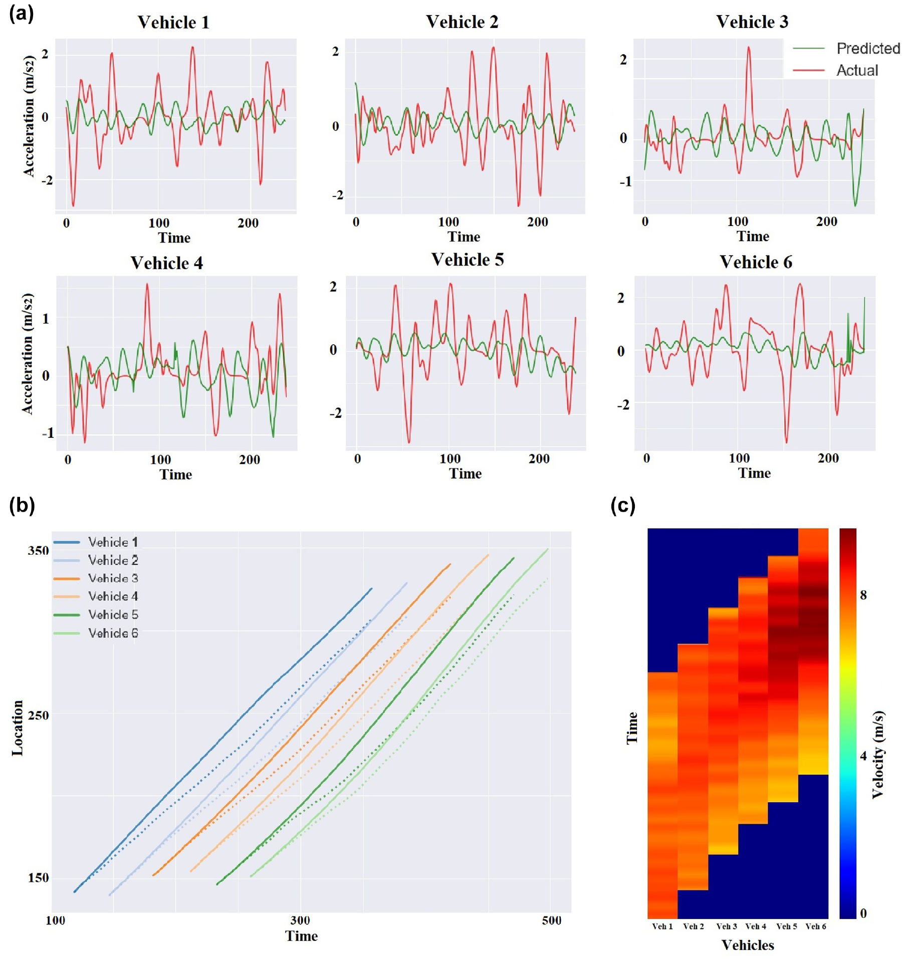
The global level simulation results of an average performing car-following (CF) model with mean square error (MSE) = 1.08, negative headway = 0%, negative velocity = 0%, and jerkiness = 9.4. (a) the acceleration trajectories of six vehicles in a platoon, (b) the location-time diagram, and (c) the spatiotemporal diagram.
The global level results are reported in the bottom part of Table 3. ANOVA test is performed to find the significance of performance differences between the CF models. The test does not find sufficient evidence of significant performance difference between the CF models for MSE, percent negative headway, and percent negative velocity. However, the test revealed a significant mean difference in the level of jerkiness. The z-test illustrates that the all-surrounding-vehicles and adjacent-lanes CF models generate traffic flow with significantly more jerky behaviors (i.e., less smooth) than the other models, and the classic CF model shows significantly smooth traffic flow.
Sensitivity Analysis
The CF models’ performance could be biased to the deep-RNN’s hyperparameters (e.g., network size and learning rate). A sensitivity analysis was conducted on the hyperparameters at the local and the global levels. The goal of this sensitivity analysis is to investigate whether a change in the hyperparameters could change the conclusions about the five CF models’ relative performance.
The sensitivity analysis was performed for the number of cells at each hidden layer, learning rate, and the number of hidden layers. The code has been run with three different values for each hyperparameter. The sensitivity analysis is executed only for the middle-lanes dataset because it has the largest number of observations among the other lanes. Performing sensitivity analyses on all lanes was not feasible because of the long processing time and computational constraints. Thus, the results of this section are limited to the middle lane. The results are reported in Table 4. The table’s top section shows MSE for different model configurations with different numbers of cells, learning rates, and hidden layers at the local level. The last column presents p-values for the ANOVA test. The best-performing configuration (i.e., the base configuration) is selected and used in this study. Since the p-values are much higher than the Benjamini–Yekutieli significance level, the null hypothesis (i.e., there is no performance difference between the CF models) is not rejected. The result illustrates that, although the models have slight performance differences, these differences are not statistically significant. All the configurations lead to the same conclusion that there is no sufficient evidence of significant performance differences between the CF models. This result indicates that the CF models’ comparison at the local level is robust, and the hyperparameters do not influence the comparison’s results.
Sensitivity Analysis for Deep Recurrent Neural Network (Deep-RNN)’s Hyperparameters
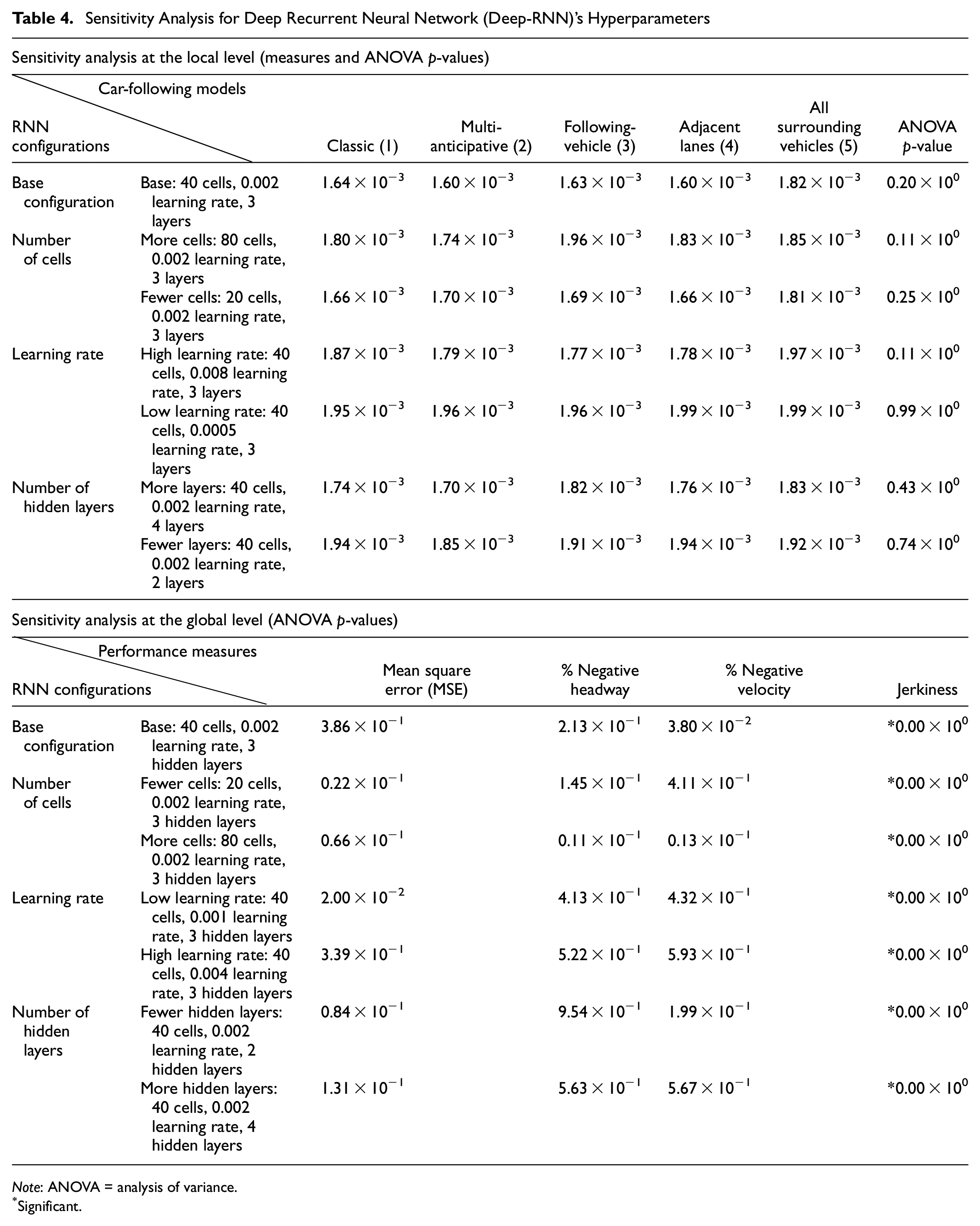
Note: ANOVA = analysis of variance.
Significant.
The result of sensitivity analysis at the global level is shown in the bottom section of Table 4. ANOVA test is used to evaluate the robustness of the comparison between the CF models. The table does not report the measures’ values (e.g., MSE and percentage negative headway), instead ANOVA p-values are reported for all configurations because of the space limit. This information is available from the authors on request. The best-performing configuration is the base configuration at the global level. The p-values are higher than the Benjamini–Yekutieli significance level, except for the level of jerkiness. Despite changing the hyperparameters, the ANOVA results for MSE, percent negative headway, and negative velocity are always non-significant, and the results for jerkiness are always significant. The sensitivity analysis illustrates that the deep-learning configuration does not influence the conclusions. The hyperparameters may cause small variations in CF models’ relative performances, but these variations do not significantly change the comparison’s results.
Discussion
Several studies have claimed multi-anticipative or adjacent-lanes CF models outperform classic CF models ( 8 , 10 , 12 , 14 , 16 ). However, not enough evidence was found of significant performance differences between a classic CF model and multi-anticipative or adjacent-lanes CF models in this study. This inconsistency might be caused by several factors ignored in the previous studies (e.g., bias in modeling, and testing with real-world data). First, parametric CF models may cause bias in modeling and influence outcomes of the comparison. This study is the first study in the literature using assumption-free data-driven CF models with no pre-assumption on driving behavior. Second, every human-related study should be validated by real-world data. Numerical simulations and stability analyses may provide initial insights on CF behavior; however, they should not be substituted for validation with real-world traffic data. Additionally, a large enough sample of traffic data should be used to achieve a robust comparison. Like previous studies, this study has found some performance differences between the models, but the differences have not been found statistically significant. The studies which compared average performances between the models should perform statistical analyses to test the significance of performance differences.
There might be two concerns about the proposed framework. First, since CF models have a different number of inputs, the deep-RNNs’ architectures in the input layer are not identical, and the CF models are not compared in a fair condition. Second, deep-RNN’s size should be adjusted by input size (i.e., a larger RNN network for a larger input size). At first, the authors agree that a change in the number of inputs changes the input layer’s size. This is an important issue for shallow neural networks (i.e., single-layer). However, the impact of the input layer is decreasing as the number of hidden layers increases. This study uses a multi-layer RNN with three hidden layers, which minimizes the impact of the input layer’s impact on the final output.
It may be argued that a CF model with a larger input size needs a larger deep-RNN (i.e., more cells or more hidden layers) to learn from data. So, using the same size deep-RNN for all CF models may cause underfitting and unfair comparison. The authors used a dynamic validation-based stop-condition to tackle this issue, instead of a fixed number of training epochs. In the dynamic stop-condition, the deep-RNNs are trained until they reach maximum learning capability where the training is stopped. This stop-condition prevents underfitting and provides a fair amount of training for all CF models with different input sizes. CF models with a large input size would reach the non-improving condition after more epochs of training. While CF models with a small input size reach the non-improving condition after few training epochs. More importantly, the sensitivity analysis is performed to ensure that deep-RNN’s size (i.e., the number of layers or cells) does not influence the comparison’s outcome. The sensitivity analysis tested cell sizes from 20 to 80 and hidden layers from 2 to 4. The result demonstrates that changing deep-RNN’s size does not change the conclusion. Thus, CF models with a larger input size do not perform better when deep-RNN’s size increases in this study.
It should be clarified that this study does not conclude or suggest that surrounding vehicles have no impact on subject vehicles’ behavior (e.g., speed or headway choice). Previous studies have performed statistical analyses and illustrated that the surrounding vehicles influence subject vehicles’ behavior ( 13 , 15 ). This study concludes that incorporating surrounding vehicles’ information in CF models does not “significantly improve the performance of CF models.” In other words, the subject and preceding vehicles’ information would be sufficient to develop a well-performing CF model. Adding information from the other surrounding vehicles does not cause a significant improvement in the model’s performance. The surrounding vehicles may influence drivers’ CF behavior, but incorporating the surrounding vehicles’ information in CF modeling does not improve its performance. This effect could be caused by several potential reasons (e.g., high correlations between preceding vehicles’ attributes and the surrounding vehicles’ attributes), which need further investigation in future work.
Conclusion
This paper introduces two new CF models. The following-vehicle CF model in which information from the vehicle behind the subject vehicle is considered. The second model is the all-surrounding-vehicles CF model. This model attempts to improve the performance of CF models by combining multi-anticipative and adjacent-lanes CF models.
This study proposes a fair and comprehensive comparison framework for CF models. A fair comparison framework has been developed to minimize the risk of randomness and bias in the comparison. The framework performs a detailed comparison between the models at the local and global levels.
In this study, sufficient evidence has not been found of a significant performance difference between the classic CF model and the multi-anticipative CF model. The following-vehicle CF model has been found to have similar performance to the multi-anticipative model, with no significant difference from the classic model. The adjacent-lanes CF model has illustrated variation in performance in different lanes. While it outperforms the other models on the middle lanes and right-most lane, it significantly underperformed on the HOV lane. The global level comparison also demonstrated that the adjacent-lanes CF model generates significantly jerkier (less smooth) flow than the other models. The all-surrounding-vehicles CF model has significantly underperformed the other CF models in relation to accuracy and smoothness. The all-surrounding-vehicles CF model is not recommended for traffic modeling.
This paper provides some opportunities for future studies. The inconsistencies between this research and the previous studies are valuable opportunities for future studies to investigate the factors causing these inconsistencies. The current study only investigated passenger vehicles’ behavior; however, heavy-duty vehicles’ behavior and mixed-traffic flow (i.e., passenger and heavy-duty vehicles) could be studied in the future. This paper also could be extended to integrate CF and lane-changing models in a single deep-learning model. This integrated model could investigate how considering/ignoring surrounding vehicles could affect the model’s performance in different lanes. Future studies could also apply feature engineering and feature selection techniques (e.g., autoencoders, principle component analysis) to find an optimum set of inputs for CF models. Quality of data could affect the models’ learning process and reduce the robustness of the conclusions. This study used the reconstructed NGSIM dataset, which is one of the high-quality available traffic datasets. This study may be re-conducted when traffic data with higher quality becomes available in the future.
Footnotes
Author Contributions
The authors confirm contribution to the paper as follows: study conception and design: S. Vasebi, Y. Hayeri; data collection: S. Vasebi; analysis and interpretation of results: S. Vasebi, Y. Hayeri; draft manuscript preparation: S. Vasebi, Y. Hayeri, P. Jin. All authors reviewed the results and approved the final version of the manuscript.
Declaration of Conflicting Interests
The author(s) declared no potential conflicts of interest with respect to the research, authorship, and/or publication of this article.
Funding
The author(s) received no financial support for the research, authorship, and/or publication of this article.