
Abstract
For transportation system analysis in a new space dimension with respect to individual trips’ remaining distances, vehicle trips demand has two main components: the departure time and the trip distance. In particular, the trip distance distribution (TDD) is a direct input to the bathtub model in the new space dimension, and is a very important variable to consider in many applications, such as the development of distance-based congestion pricing strategies or mileage tax. For a good understanding of the demand pattern, both the distribution of trip initiation and trip distance should be calibrated from real data. In this paper, it is assumed that the demand pattern can be described by the joint distribution of trip distance and departure time. In other words, TDD is assumed to be time-dependent, and a calibration and validation methodology of the joint probability is proposed, based on log-likelihood maximization and the Kolmogorov–Smirnov test. The calibration method is applied to empirical for-hire vehicle trips in Chicago, and it is concluded that TDD varies more within a day than across weekdays. The hypothesis that TDD follows a negative exponential, log-normal, or Gamma distribution is rejected. However, the best fit is systematically observed for the time-dependent log-normal probability density function. In the future, other trip distributions should be considered and also non-parametric probability density estimation should be explored for a better understanding of the demand pattern.
To improve mobility, researchers study ways of “shaping travel demand.” Many different strategies can be considered, and most involve the reduction of distances traveled by motorized vehicles, for example, by reducing the number of motorized trips or increasing vehicle occupancy level for the motorized trips ( 1 ). Transportation demand in a road network is traditionally stored in origin–destination (OD) matrices, where each cell represents the number of vehicle trips between each OD pair. Depending on the duration of the time interval, the OD matrix is said to be static (long period of time) or dynamic (short period). However, the estimation of OD matrices is generally not very accurate because of the limited data available. In fact, the problem is known to be under-determined when one tries to estimate OD matrices from link flows. Further, the estimation of dynamic OD matrices is very computationally expensive. Nevertheless, demand calibration or modeling is a key component in any traffic flow model to model traffic congestion accurately and propose adequate operational strategies to alleviate it.
Recently, a new paradigm for transportation system analysis has been introduced where the spatial dimension is relative. The idea is to disregard the network topology and use space as a relative distance to the destination ( 2 , 3 ). In this new paradigm, the travel demand is described by the number of trips initiated at any given time and the trip distance distribution (TDD) of these trips ( 4 ). This demand definition is a direct input (or assumption) of the so-called bathtub models (2–5), which have been gaining interest in recent years among the research community. While the supply side of the bathtub models has had a lot of attention in the literature, the calibration of demand has been overlooked. Several studies have highlighted the important role of trip distance (in this case at a regional level) on the accurate prediction of traffic dynamics (6–8). More recently, it has been observed, based on mobile phone data, that the mean trip distance changes over the day ( 9 ), which contradicts the common assumption of time-independent TDD for the bathtub model ( 2 , 3 , 10 , 11 ).
In transportation science, the trip distance of the users is a fundamental variable that is needed for studying different aspects. For example, it is an important input in the “trip distribution” step of the four-step model, since it represents a measure of travel impedance. In the past, the data available to estimate the trip distance has been sparse, because it was collected through surveys. However, in recent years, other ways to collect the trip distance information have become available from mobile phone data (12–14) and GPS traces ( 15 , 16 ). Several empirical studies have reported different TDD, such as log-normal distribution ( 14 , 17 , 18 ). These new technologies for data collection will make it possible to obtain larger data sets and a more accurate estimation of demand. However, the collection of such detailed information might lead to concerns about users’ privacy. When considering the new relative space paradigm for transportation, the data requirements are lower and it might be easier to guarantee privacy because only two variables should be collected. Thus, GPS traces and mobile phone data present a potential data source to estimate the demand for the new transportation paradigm. However, there is no systematic calibration procedure in the literature for this demand definition.
In summary, the study of TDD is gaining interest in the research community, both from the practical and modeling perspectives. TDD jointly with the trip initiation rate defines the travel demand and dictates the congestion dynamics in a road network. It is natural to think of the demand as a joint distribution of trip distances and departure time, although this concept is rather novel ( 4 ). This paper proposes a trip demand estimation methodology for such joint distribution. The method is then used to calibrate the TDD of for-hire vehicle trips reported by the transportation network providers in Chicago, for two common TDD assumed in the literature and a generalized function. Through statistical testing, the hypothesis that TDD is time-independent is rejected. The hypothesis that it follows any of the distributions considered in this paper is also rejected, which reveals the necessity of further studying the joint distribution of trip distances and departure time, since the common assumptions in the literature are not supported, at least for the data set considered in this paper.
The rest of the paper is organized as follows. The next section presents a literature review of TDD assumptions and models. Then, the definition of the joint trip distance and departure time distribution are presented and the methodology for its calibration is proposed. Later, an overview of the data used is presented and the time-dependency of the TDD is established through hypothesis testing. Then, both calibration and validation of three different time-dependent probability density functions are performed, and the results are discussed. Finally, a discussion on the contributions, limitations, and practical implications of this study is presented, and the paper concludes with a short summary.
Literature Review
This section will first summarize the assumptions on TDD for bathtub models. Then, some existing models and empirical calibrations of TDD are reviewed.
Trip Distance Assumptions in Bathtub Models
The “bathtub model” was a term proposed by Vickrey ( 2 , 3 ) to describe an aggregated model capturing the completion of trips in the city as a function of the number of vehicles in it. The dynamics are described by a conservation equation of the active vehicles in the system. The supply side of the bathtub models has been studied extensively in the literature, for example, through the network fundamental diagram calibration, also known as the macroscopic fundamental diagram. Demand is another important input of the bathtub model. However, the estimation of the TDD has been largely overlooked in the bathtub model literature. This paper aims to fill this gap by defining and estimating the time-dependent TDD. This will also help us to have a better understanding of the demand.
There is a special case where the traffic dynamics can be modeled with a simple ordinary differential equation. This was first derived assuming that the trip distance of the users in the network follows a (time-independent) negative exponential (NE) distribution ( 2 , 3 ), such as

where
Other TDD have been assumed in the literature for bathtub models, for example, the same trip distance for all travelers ( 5 ). This model with homogeneous users is often referred to as the “basic bathtub model.” Recently, the so-called “generalized bathtub model” was derived for any given TDD ( 4 ). The completion rate of trips for the generalized bathtub model depends on the distribution of remaining trip distances ( 4 ).
The so-called “trip-based model” ( 5 , 22–24) is developed as a reformulation of the bathtub model, where the objective is to track individual users’ trip progression. Most of these studies consider constant trip distances and thus are equivalent to the basic bathtub model. A framework to determine explicit distributions of travel distances has been proposed based on information on vehicle trips in the city network through sampling of a set of (virtual) trips ( 7 ). These distributions were assumed to be time-independent but the probability density function was not calibrated. Later, the framework was extended to assume that a single trip can change its route depending on the traffic conditions. However, in this paper, it is assumed that the trip distances are fixed for individual vehicle trips.
In summary, there are several assumptions in the literature on TDD for bathtub models. Many researchers have assumed constant TDD ( 5 , 24 , 25 ), and others have assumed NE distribution either explicitly ( 2 , 3 ) or implicitly ( 10 , 11 ). In this paper, whether the trip distance is time-independent and whether the trip distance follows a NE distribution will be tested.
Existing TDD Models
In general, trip distance (or trip length) is studied through regression models based on population density and other demographic characteristics (
13
). The distribution step of the four-step model has traditionally been done based on gravity models, using a functional distribution of the travel impedance, for which parameters are calibrated subsequently. The travel impedance is in most cases defined by the trip distance. Thus, different functional forms of TDD have been considered in the literature. The most popular functions are NE, power-law, or a combination as
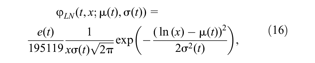
The calibration in TDD for gravity models is traditionally done with limited survey data, thus the results were not very accurate. More recent findings by Colak et al. ( 14 ) based on mobile phone data suggest very interesting similarities between TDDs across the five cities analyzed. In particular, they concluded that the straight line distance between origins and destinations for commuting trips follows a log-normal distribution, that is,
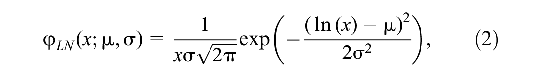
where
All these empirical studies aggregated the trip distances across hours (or days) and calibrated a single distribution. This means that their studies (indirectly) assumed that the TDD is time-independent. However, it is important to consider trip distance variation for micro-simulations ( 6 ). For this reason, the present paper defines the joint distribution of departure time and trip distance ( 4 ) as the demand and proposes a method to study and calibrate the time-dependent TDD. Very recently the variations in mean trip distance (MTD) across peak and off-peak hours have been studied by Paipuri et al. ( 9 ). They observed, with empirical data, that MTD changes over time. However, the trip distance analysis was based on regional paths, that is, single trips were “cut” into regions and for each region the TDD was obtained. Therefore the analyzed TDD were dictated by the topological features of the city network and the network partitioning. There are three main differences between this paper and Paipuri et al. ( 9 ). First, this study considers the trip distance analysis of the whole trips, which allows us to study the demand, instead of studying the distribution of partial trip distances in regions that have been defined for the purpose of modeling. Thus, the present approach is more generic and the study of the TDD can serve other purposes than being the input of a bathtub model. Second, this study assumes a continuous TDD that is time-dependent and the parameters of three assumed distributions are calibrated, based on data. On the other hand, Paipuri et al. ( 9 ) do not present any calibration of TDD, and the time variation is only studied and discussed for the MTD. Finally, the present paper studies TDD through standard statistical hypothesis testing, which allows us to draw conclusions by rejection of certain hypotheses, rather than only by looking at graphical representation of the data.
Methodology
It is assumed that the TDD is time-dependent, as discussed in Thomas and Tutert ( 17 ). However, it is argued here that this time-dependency might be on a shorter time-scale, that is, within a day or across days, instead of considering a change over years. In the following, the time-dependent TDD is defined as a mixed continuous-discrete joint distribution.
Definition of Joint Probability Function
The concept of joint probability density function for trip lengths and time is a very natural concept, but a very novel one (
4
). A joint probability function defines the likelihood of two events occurring together at the same instant. This joint distribution can be discrete, continuous, or a mixture. If the joint distribution of trip distance and departure time,
There is no empirical study that has tried to calibrate this joint distribution
From the axiom of probability the joint probability density function can be defined mathematically as

where
Time being a discrete variable, the marginal probability of trip generation is defined as

where

This mixed joint distribution based on discrete time intervals and continuous trip distance
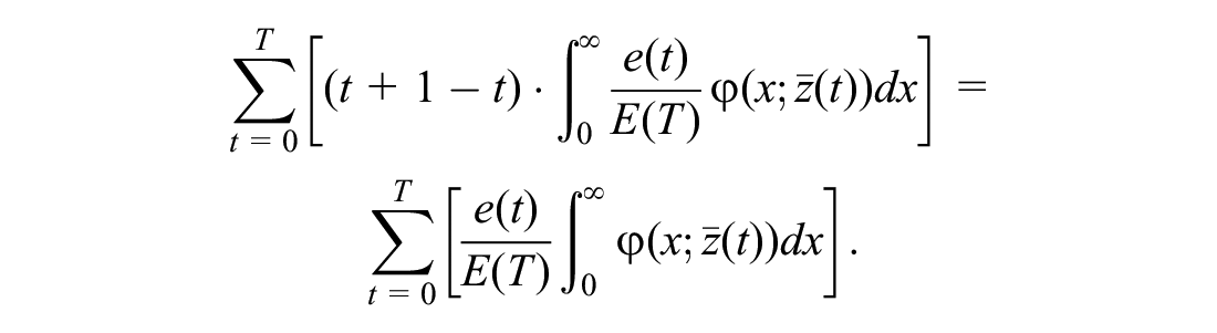
Clearly, the volume is one since
Hypotheses Considered
In this paper, the time-dependency is studied through Hypothesis 1.
The joint probability distribution is then studied by considering three different possible functions. The NE distribution (Equation 1) and the log-normal distribution (Equation 2) are considered, since other empirical data were calibrated under that assumption ( 14 , 28 ). Moreover, a Gamma distribution is also considered,

where
If Hypothesis 1 is rejected, the joint probability functions defined above will be considered to be time-dependent. Hypothesis 2a, 2b and 2c will then be tested with the following null hypothesis (
These functions are presented here:

which has a single time-dependent parameter: the average trip length
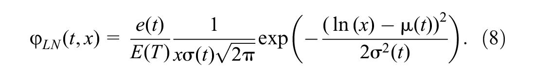
which has two time-dependent parameters:
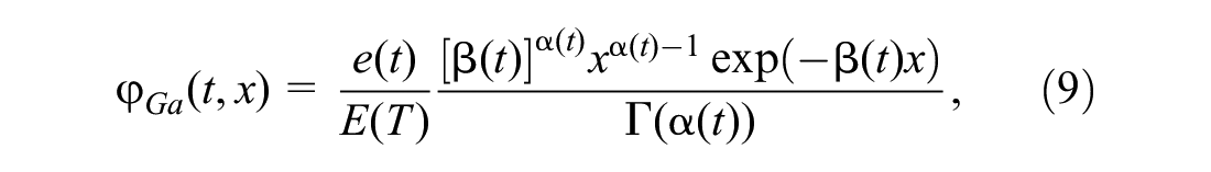
which also has two time-dependent parameters
In this paper, trips are aggregated on an hourly basis, creating the discrete time variable
The rest of this section will explain the procedure of the calibration-validation method. For each hour of the day, the trips will be randomly divided into two samples: one calibration sample used for the maximum likelihood estimation of parameters; and one validation sample to perform statistical tests.
Calibration: Maximum Likelihood Estimation
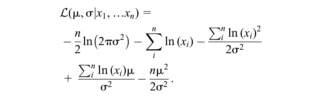
The calibration will be based on the maximum likelihood parameter estimation method. This method estimates the parameters of a given distribution from a sample of trips, for example,

which is maximized by solving
For the NE function (Equation 7) the parameter
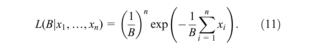
Maximizing Equation 10 with the likelihood in Equation 11 leads to
Thus, the maximum likelihood estimators are

and

The same procedure could be applied to find the Gamma maximum likelihood estimators, but to solve
Validation: Kolmogorov–Smirnov Tests
To test whether the probability distribution of a sample follows a reference probability distribution, the Kolmogorov–Smirnov (KS) test can be used (
30
,
31
). There are two types of KS test: one-sample test and two-sample test. In the first, the null hypothesis,

where

where
For the two-sample KS test, the null hypothesis,

where

Empirical Data
Data Overview
The data source of this paper corresponds to the information that transportation network providers (that is, rideshare companies) in the city of Chicago have collected since late 2018. This data is publicly available at https://data.cityofchicago.org/Transportation/Transportation-Network-Providers-Trips/m6dm-c72p. Each trip recorded has a unique identifier and information about the trip distance (in miles), duration (in seconds), starting and ending times (reported in 15 min intervals, by rounding the actual time to the nearest interval), trip fare and tip, and information whether other trips were pooled. The trips’ origins and destinations are zone-based, corresponding to the 77 community areas in Chicago, depicted in Figure 1. We are not interested in including the trips with origin or destination at the airport or other peripheral areas. For this reason, a limited (more or less convex) area is considered for the analysis, represented in yellow in Figure 1.

City of Chicago community areas. Zone of interest in yellow.
The data is cleaned to ensure that the trips recorded are meaningful, that is, trips that lasted for less than 10 s or with average speeds higher than 80 mph or lower than 1 mph are discarded from the data set. The data selected for this paper are trips that took place in 2019 that had both pick-up and drop-off points in the yellow community areas marked, which corresponds to 45 community areas and 72.7 million trips. The millions of trips initiated and ended in each community area and their associated mean distances are depicted in Figure 2. Clearly, the average trip distance is location-dependent. However, the analysis of location-dependent trip distance is outside the scope of this paper. Recently, the spatial variation of ride-hail trip demand of this data set has been analyzed ( 32 ). Notice that the areas with higher number of trips correspond to the areas with lower average trip distance. These community areas (6, 7, 8, 22, 24, 28 and 32) also correspond to the downtown of Chicago, where many trips are likely to originate and end in the downtown area itself, and are short trips.
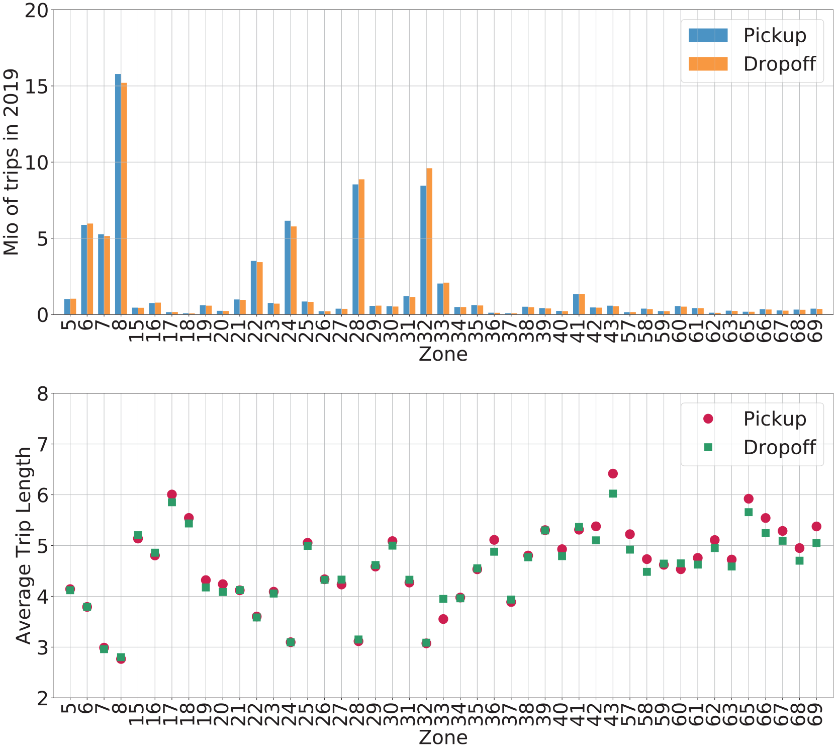
(a) Millions of trips started/completed in each community in the zone of interest, and (b) associated average trip distance (miles).
The data analysis in this paper is based on two different samples of trips from the data described. The first set of data analyzed will be all the trips over a given week. In particular, the trips that took place during week 11 are analyzed, since it corresponds to the week of 2019 with most trips recorded. This sample has a 1.63 million trips with average trip distance of 3.47 miles and standard deviation of 2.80 miles. For this set, the trip generation rate and the evolution of MTD over time will be analyzed in the following subsection. This will be done to study Hypothesis 1. In the next section, the time-dependent joint distribution will be estimated for March 13, 2019 (i.e., Wednesday of week 11). This day had a total of 195,119 trips with average distance of 3.53 miles and standard deviation of 2.85 miles. As explained in the previous section, the estimation of the density function of trip distances will be made per hour. Each hour’s data will be split into two random equally large data samples, one for calibration and the other for validation. Finally, a larger data sample will be also considered in next section (∼3.64 million trips) to perform further calibration-validation analysis and study the variation of TDD over a single day and across days.
Time-Dependent Trip Distance
In this section a detailed analysis of the demand over time is presented. The data sample used corresponds to the trips recorded in week 11 of 2019. As expected from common knowledge, the trip generation at different times of day is not the same, see Figure 3, a and b , where the trip initiation for the different days is depicted with respect to time. However, the underlying TDD could potentially be time-independent. A necessary condition for the trip distribution to be time-independent is that the average trip distance is time-independent. Therefore, we will do hypothesis testing on the MTD for each hour of data. A first look into the average trip distance over time in Figure 3, c and d , suggests that the average trip distance might be time-dependent. To test this, a one-way analysis of variance (ANOVA) test will be used, considering the following null hypothesis:
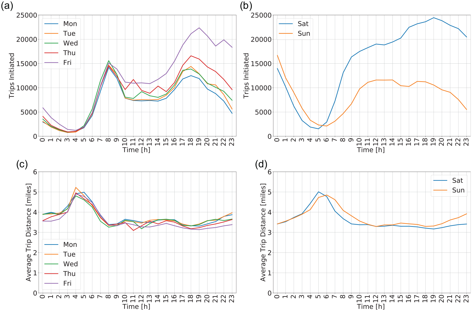
Trip initiation and distance analysis in zone of interest for week 11 of 2019: (a) trip generation at different times of day on weekdays, (b) trip generation at different times of day on the weekend (Saturday and Sunday), (c) average trip distance of trips initiated in each hour on weekdays, and (d) average trip distance of trips initiated in each hour on the weekend.
Each day’s MTD represents a data point for the groups “hour-of-day.” This leads to 24 sets of data and five data points in each group. It is verified that the assumption of normal distribution and homogeneity of variances are met for all 24 sets of data. Considering Hypothesis 3, the statistic for the ANOVA test is 37.9 and p-value is
Another observation to highlight from Figure 3 is that the average trip distance is longer for the hours of day when the trip generation is lower. This is so for all the days of the week. Notice that this relation is consistent with the observations in the previous subsection (i.e., Figure 2) where regions with lower production and attraction of trips had longer average trip distances. It seems that during the early morning, when the demand is low (especially between 4:00 and 7:00 a.m.), longer trips are more likely to happen than during other times of the day, increasing the mean value. The reasons for this relation may be the nature of the demand. For example, it is natural that people with long trip distances would choose transportation mode other than ride-hailing, especially during peak congestion time. Another possible explanation is that riders with longer trip distances try to avoid the early morning congestion by requesting a for-hire trip earlier. Alternatively, another reason why these longer trip distances are not observed in the afternoon is that these commuters might use other modes of transportation that were unsafe (or not available) in the early morning. Finally, this relation might be explained with spatial variations of trip distances, as reported in Figure 2. All these assumptions should be tested in future studies.
The MTD and standard deviation for each hour are compared pairwise between weekdays and weekends in Figure 4. The figure also shows that the standard deviation is systematically lower than the MTD, which indicates that the assumption of NE distribution ( 2 , 3 ) might not be adequate, since the expected value and standard deviation are equal in a negative exponential distribution. This will be tested in the subsections “Joint Distribution for Single Day” and “Calibration-Validaton of Tuesday and Wednesday Subsets.”
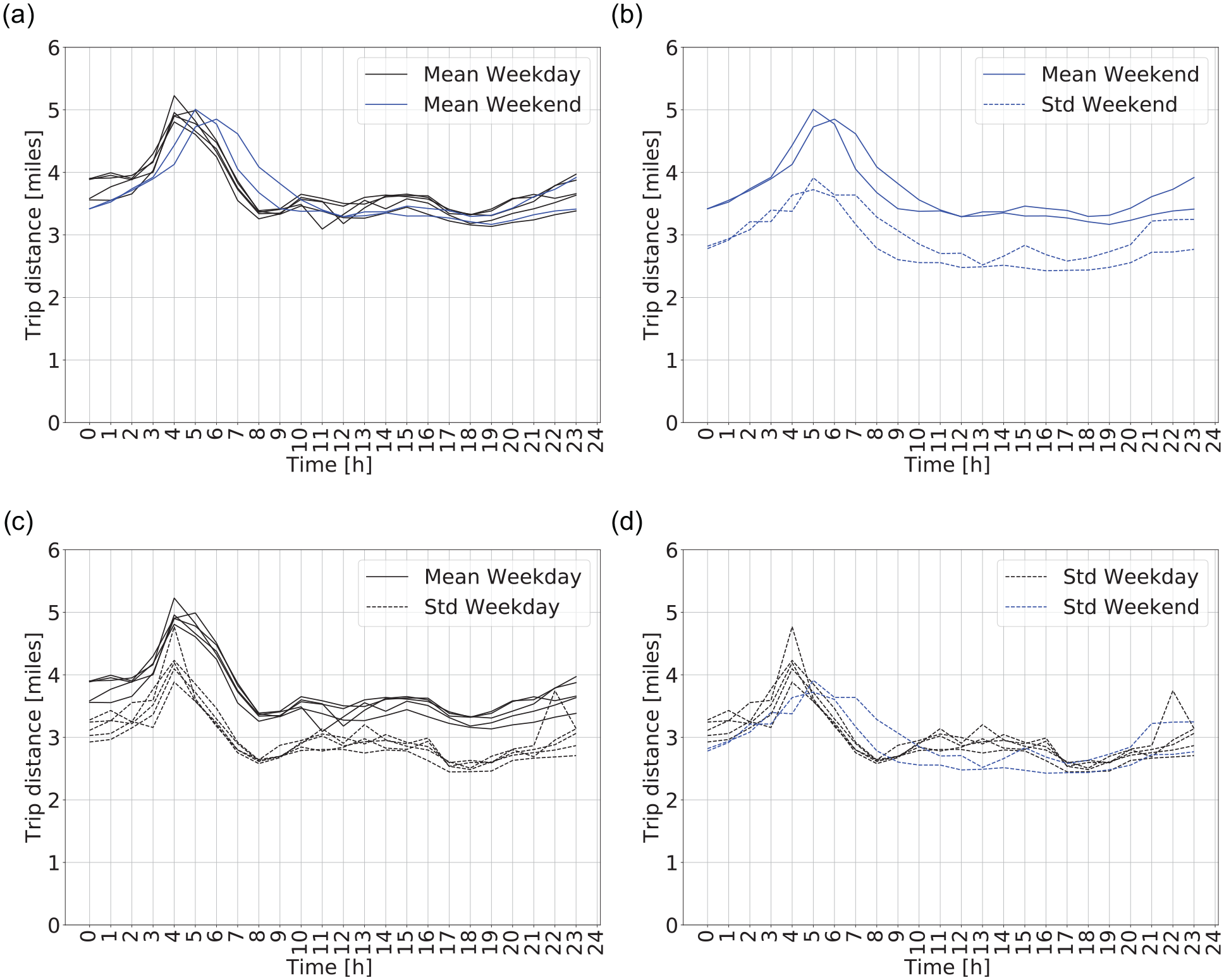
Trip distance mean and standard deviations over time for weekdays (black) and weekends (blue): (a) compares mean trip distance between weekdays and weekends, (b) compares mean and standard deviation of trip distance for weekends, (c) compares mean and standard deviation of trip distance for weekdays, and (d) compares standard deviation of trip distance between weekdays and weekends.
The aggregated trip distance probability mass function (PMF) across all weekdays is presented in Figure 5a, while individual days’ PMF are presented in Figure 5b for completeness purposes. These aggregated mass functions for the whole day have a similar form to the Gamma or log-normal probability density functions. However, the estimation of these aggregated distributions is not the purpose of the paper, because we have rejected Hypothesis 1 and concluded that TDD is time-dependent. In the next section time-dependent calibration-validation analysis will be performed.
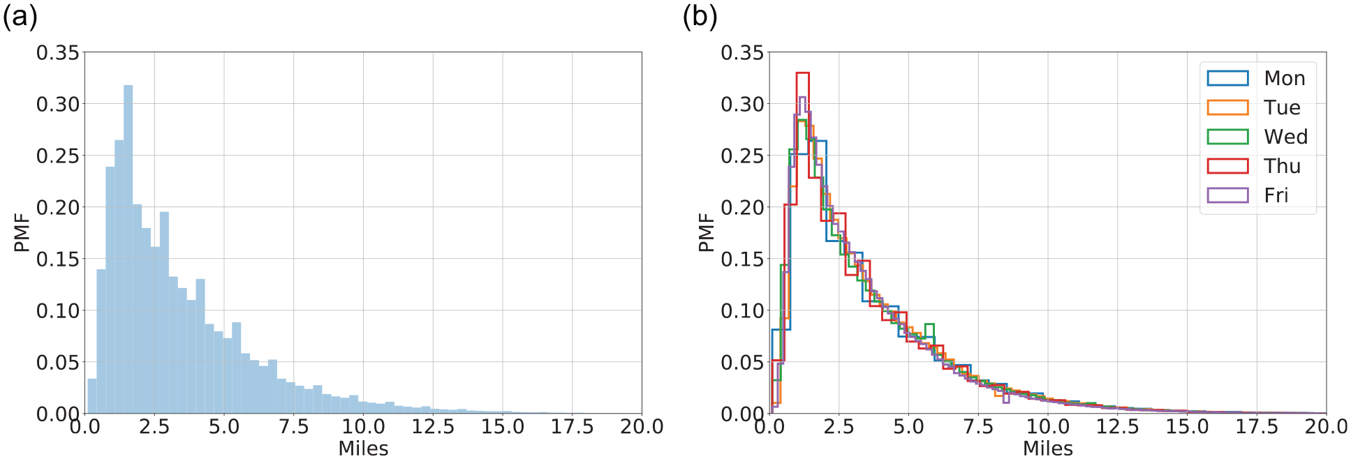
Trip length empirical probability mass functions for (a) all days of week 11 of 2019 and (b) individual week days, that is, Monday, March 11 to Friday, March 15, 2019.
Empirical Calibration and Validation
Joint Distribution for Single Day
In this section a maximum likelihood estimation from (Equations 7–9) is done for the March 13, 2019 trip data. First, the joint empirical PMF for that day is presented in Figure 6a, where trips have been aggregated in an hourly way and the trip distance
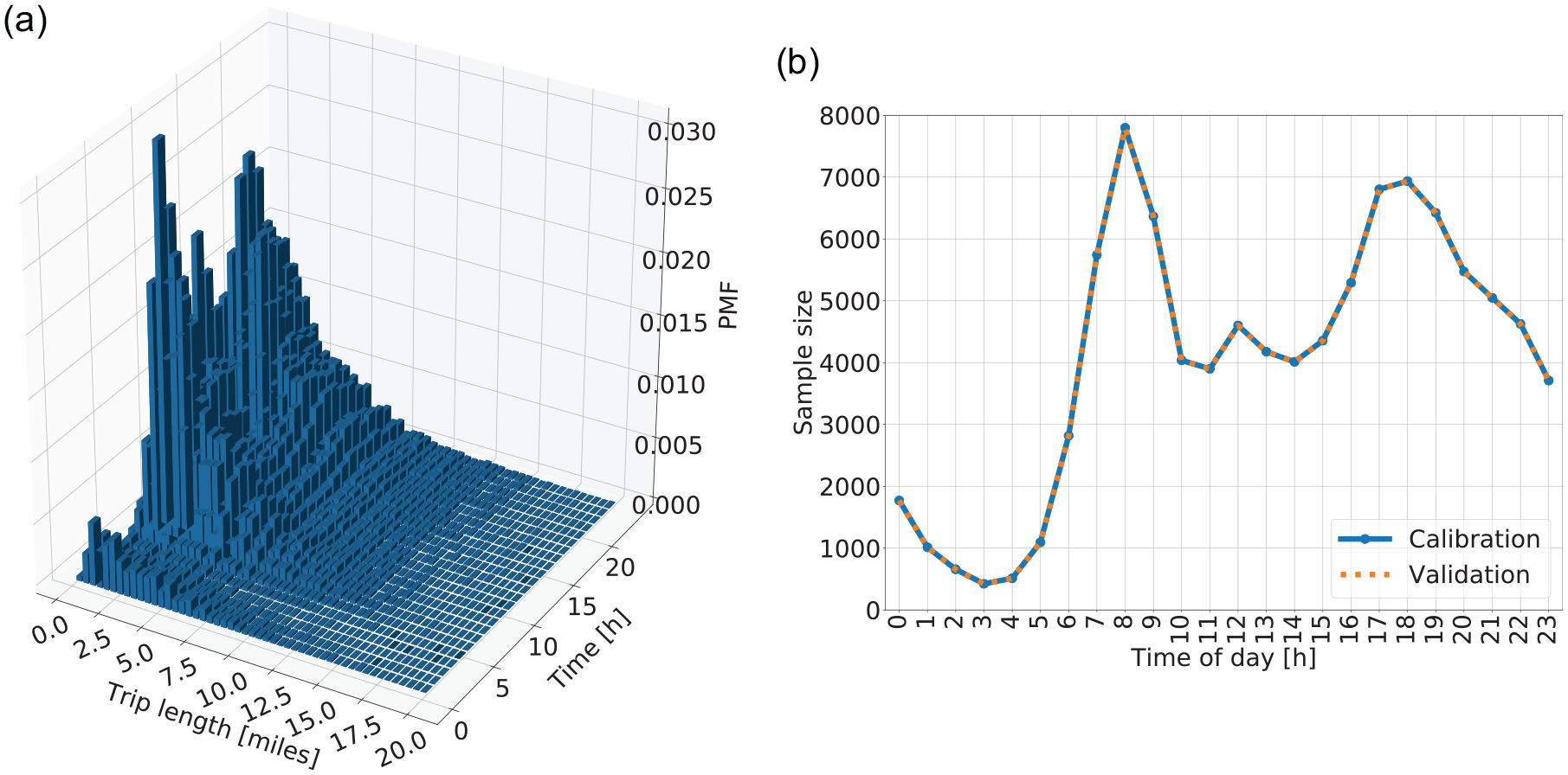
Joint distribution for trip distance and trip initiation for Wednesday, March 13, 2019: (a) empirical joint probability mass function and (b) sample sizes of calibration and validation subsets for each hour.
The parameters from the estimation for the three distributions considered are omitted here for the sake of brevity. The KS statistics (Equation 12) are presented in Figure 7 for validation purposes. The subscript indicates what is the underlying distribution, that is,
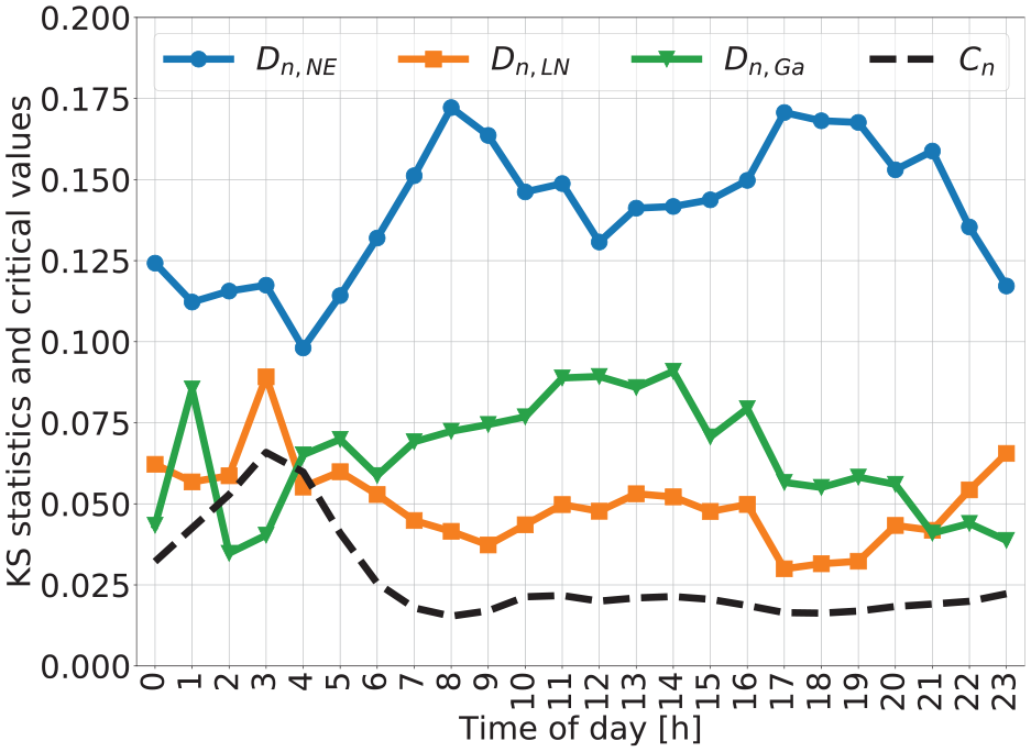
Kolmogorov–Smirnov (KS) statistic for each hourly estimation for the three different trip distance distributions (TDD) considered. Blue
Between 4:00 a.m. and 9:00 p.m., we can see that
presented in Figure 8a. For a better representation, Figure 8, b–e, present the cuts of the joint probability
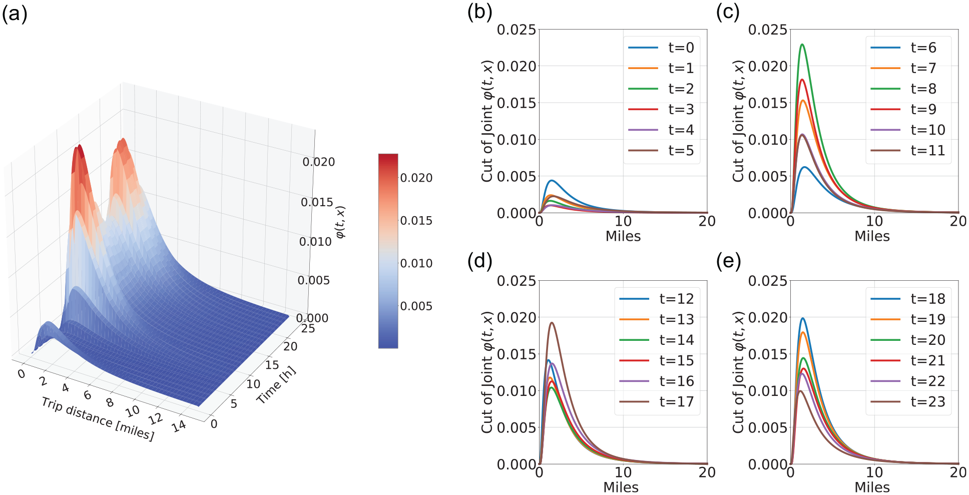
(a) Calibrated joint distribution and (b–e) cut of joint distribution represented as a curve for each hour
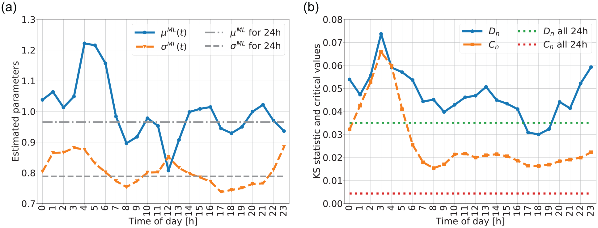
(a) Time-dependent parameters of log-normal estimated parameters and the estimated parameters for the whole day and (b) Kolmogorov–Smirnov (KS) statistic
For the sake of comparison with the aggregated TDD for the whole day, calibration and validation of the log-normal distribution is also performed (see gray horizontal lines in Figure 9a). Compared with the parameters obtained from other cities,
Time Variation Analysis
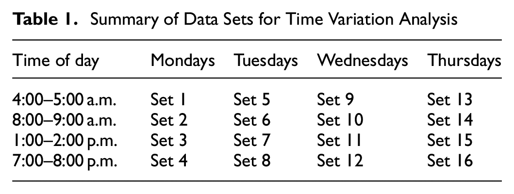
This section considers a larger data sample (from multiple days), to ensure the robustness of the results reported for a single day. Moreover, it is interesting to study whether time variation in TDD is larger across days or within days. To do so, the data collected during four different hours (two off-peak and two peak hours) for all weekdays (except Friday) in 2019 are considered. Therefore, there is a total of 16 data sets, which are labeled as in Table 1. The focus here is only on the conditional distribution estimation,
Summary of Data Sets for Time Variation Analysis
The cumulative mass function and the cross-comparison across days and hours of days is presented in Figure 10. A first look into the cumulative mass function highlights the similarity between days for each given hour. In the following, only the Sets 5 to 12 (i.e., Tuesdays and Wednesdays) are analyzed because they correspond to the days with higher reported difference in the cumulative mass functions, see Figure 10, f and i . The pairwise comparison for all 4 h is depicted in Figure 11a. The similitude between the early morning hours (4:00–5:00 a.m.) is not as evident as the other hours analyzed. Figure 11b presents the differences between the cumulative mass functions on Tuesdays for different hours of day compared with the morning peak. This figure reinforces the hypothesis in the previous section that the TDD time-dependency changes more over a single day than across days of the week.
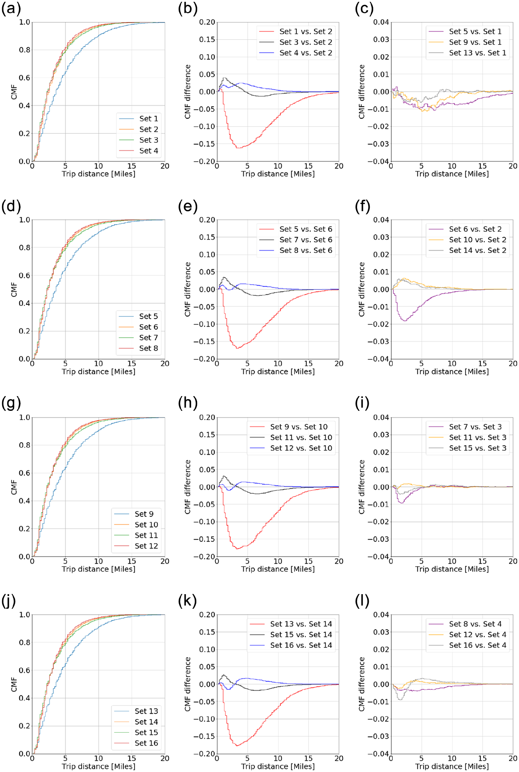
(a, d, g, j) Cumulative mass functions for the different sets of data described in Table 1, Monday–Thursday. (b, e, h, k) Difference in cumulative mass functions for a given day across time of day, Monday–Thursday. (d, f, i, l) Difference in cumulative mass functions across days for a given time: (a) Monday, (b) Monday, (c) 4:00–5:00 a.m., (d) Tuesday, (e) Tuesday, (f) 8:00–9:00 a.m., (g) Wednesday, (h) Wednesday, (i) 1:00–2:00 p.m., (j) Thursday, (k) Thursday, and (l) 7:00–8:00 p.m.
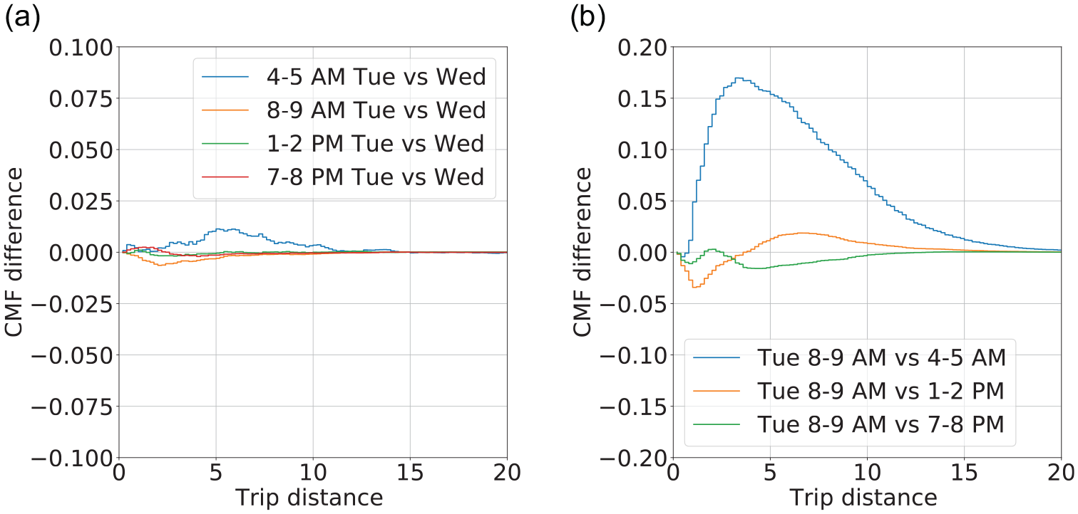
Difference in trip distance cumulative mass function (CMF) across subsets: (a) comparison between Tuesday and Wednesday, and (b) comparison within day for Tuesday data.
Two Sided KS Test
This section will consider the following hypothesis:
To test Hypothesis 4, the two-sample KS test is used. The KS statistic (Equation 14) is presented in Figure 12. In particular the data sets of Wednesday samples are tested against each other in Figure 12a; and against the data sets for Tuesday in Figure 12b. The pairs with darker color present more similitude among their cumulative distribution. The diagonal comparison in Figure 12a is ignored, since it compares the same sample. The
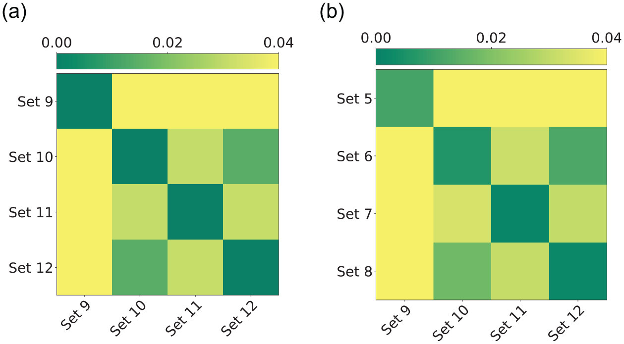
Two-sample Kolmogorov–Smirnov (KS) statistic to compare data sets. The color of each square represents the value of the KS statistic,
The diagonal terms in Figure 12b are darker than the non-diagonal squares in 12a, which indicates that the distributions from the same hour are more similar across days than the distributions of a given day for different hours. The peak hour TDDs have higher similitude than the off-peak TDDs. Furthermore, the lightest pairs, which correspond to greater differences in the cumulative distributions, are always for Sets 5 and 9, which corresponds to trips sampled at 4:00 a.m. This suggests that TDD during the early morning is notably different than the rest, as suggested by Figure 11.
Calibration-Validation of Tuesday and Wednesday Subsets
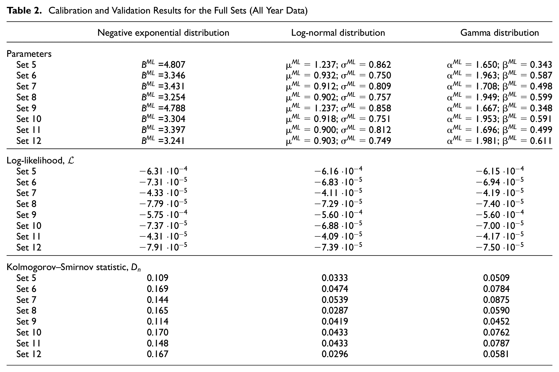
In this subsection the validation and calibration are performed, as presented in the Methodology section, on different samples of the data sets corresponding to Tuesday and Wednesday (Set 5–Set 12). The results are shown in the first part of Table 2. The log-likelihood is calculated from the calibrated data as Equation 10. From the results in Table 2 it can be seen that for each data set the maximum log-likelihood is obtained for the calibration of log-normal distribution, except for Sets 5 and 9. For these sets, the log-likelihood from the Gamma distribution fit is either greater than or equal to the log-likelihood from the log-normal calibration. Notice that the log-likelihood for the NE distribution is consistently lower than the other two, indicating a worse fit to the data.
Calibration and Validation Results for the Full Sets (All Year Data)
The KS statistic,
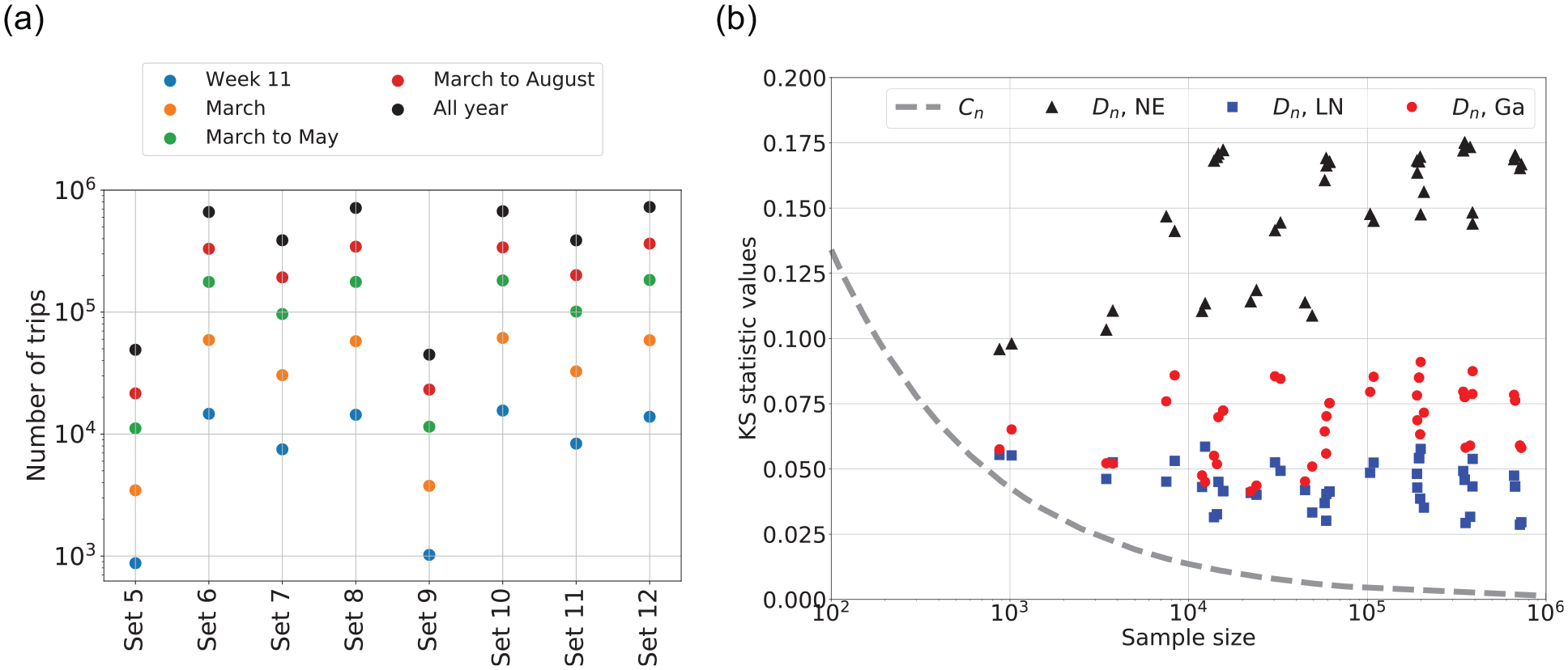
(a) Number of trips for each sample considered. Each color represents a sample of the data set during a different period of time and (b) analysis of Kolmogorov–Smirnov (KS) statistic,
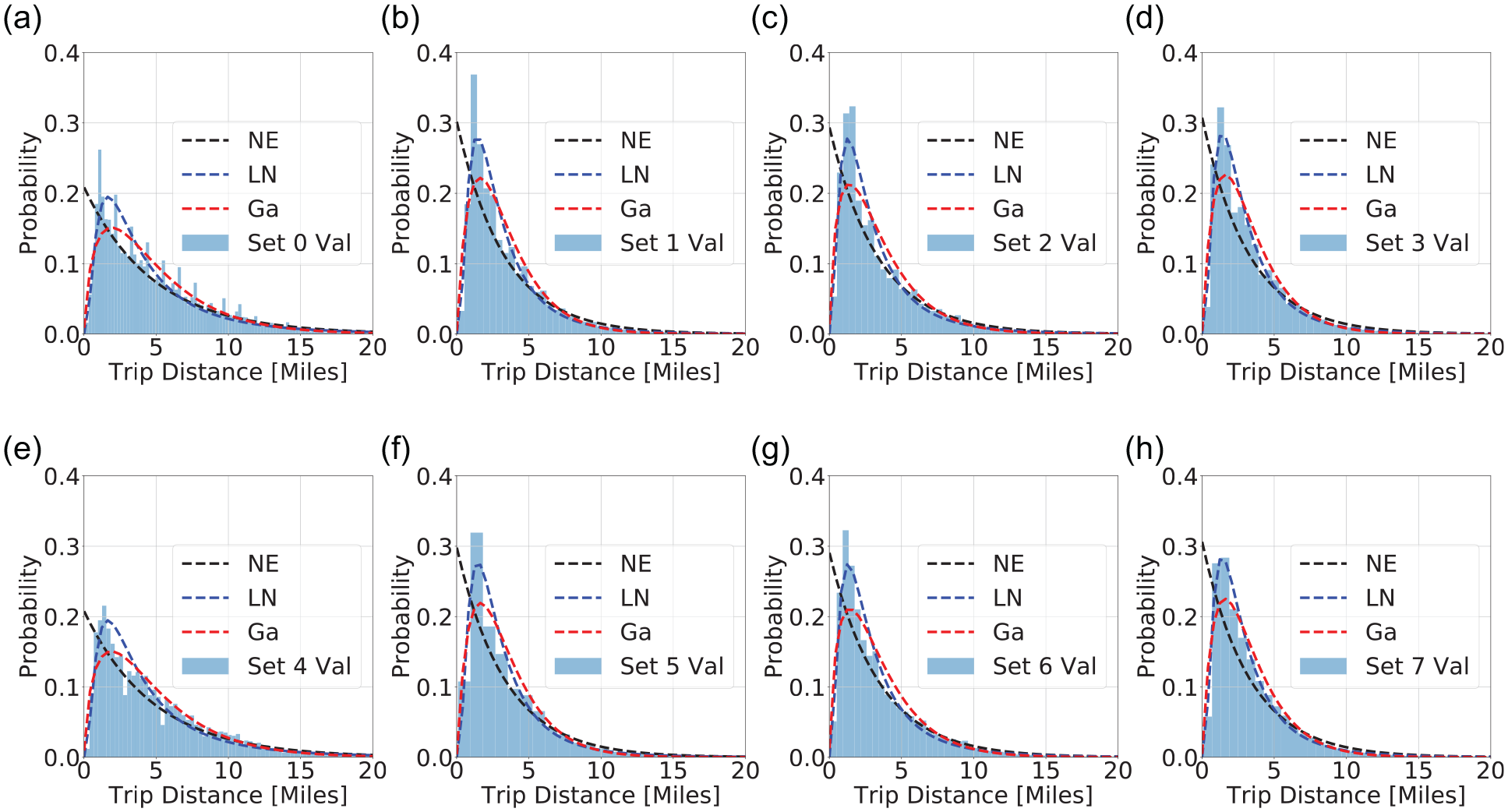
Empirical conditional trip distance distribution of validation subsets and the three maximum likelihood calibration distributions,
Recall that decay of KS critical value is inversely proportional to the square root of
Increasing the sample size increases the KS statistic for the NE distribution. In other words, the larger the sample size, the larger the difference is between the sample and NE distribution.
For the log-normal and Gamma distributions, a larger sample size does not much affect
For very large samples, the
Practical Implications, Contributions, and Limitations
Travel demand can be obtained from a travel demand model (four-step model, activity-based model, etc.) or calibrated from empirical data. In this paper, the focus is on the calibration of travel demand, especially the TDD, for transportation system analysis in a relative space dimension ( 2 – 4 ). TDD is important not only for modeling traffic congestion, but also for designing and evaluating mileage tax and other real-time operations and management schemes, including transit scheduling and distance-based congestion pricing in high-occupancy toll lanes. Further, TDD can also be used to calibrate and validate the resulting trips from activity-based models.
This paper proposes a calibration procedure to find the demand pattern empirically through the definition of the joint distribution of departure time and trip distance and maximum likelihood estimation. The Chicago data set was used to perform some statistical tests on the TDD. Most of the hypotheses considered in this paper were rejected. From Hypotheses 1, 3, and 4, the TDD should be considered time-dependent, which is consistent with another recent study ( 9 ). Testing Hypothesis 2 showed that the NE distribution is a very bad approximation for TDD, compared with the other two distributions considered (Gamma, as a generalization of NE distribution, and log-normal distribution, assumed by some researchers). Therefore, the trip dynamics of Vickrey’s bathtub model are only an imprecise approximation of the actual bathtub dynamics.
However, none of the distributions considered in this paper present a good fit for TDD. From the behavioral point of view, the distribution will depend on land use, mode choice, and departure time choice of travelers. Whether a generic TDD can be found to describe any demand pattern in any region is an open and challenging question. It is likely that a site- and mode-specific calibration is needed for each case. This highlights the importance of using the generalized bathtub model ( 4 ) over the most common bathtub models used in the literature that assume directly ( 2 , 3 ) or indirectly ( 10 , 11 ) a time-independent NE distribution of trip distances, or constant trip distances ( 5 , 25 ).
In summary, the contributions of this paper are threefold. First, it provides a systematic way to define and estimate the demand in the space–time domain, where the space dimension is with respect to the remaining trip distances. This is achieved by defining the joint distribution of departure time and trip distance as the product of the marginal and conditional distribution. Second, based on empirical data of Chicago for-hire trips, it proves through statistical methods that TDD is time-dependent, and that the variation is larger within the day than across days. Third, it rejects the hypothesis that the trip distribution follows a NE distribution (as assumed in Vickrey’s bathtub model), a log-normal distribution (considered by several authors), or the Gamma distribution. Other observations from the empirical data analyzed are that the average trip distance changes both spatially and in a temporal manner. Also, in peak periods the average trip distance is shorter, while in the early morning a higher percentage of longer trips take place. In all, a case-by-case data-based demand calibration might be needed for real-time control and traffic modeling. Even if a site-specific calibration of demand is needed, the relative space dimension paradigm allows for easier calibration and definition of demand than the traditional OD demand estimation problem in transportation analysis.
Finally, it is important to highlight that the data set used is from for-hire vehicles. For this reason, the results of this paper might not be representative of other types of trips. This study was only analyzing data from a sample of the total demand, that is, considering only one mode. Thus, to have a better understanding of the total demand pattern, further calibration of other empirical data sources is required, ideally based on privately-owned vehicle trips. Since it is conclude that the most common assumptions in the literature on TDD are not adequate for for-hire trips, the authors want to highlight the importance of carefully revising and selecting the demand assumptions for other modes. For this reason, studying empirical trip distances of other modes is important to define more adequate assumptions on the demand in the future.
Conclusions
The study of TDD has been gaining interest in the research community because of the newly available data collection technologies. This paper considers a different type of demand definition, where the geographical location of the origins and destinations is ignored. It presents a calibration and validation procedure to study the demand as a joint probability density function of trip distance and departure time. In the past, TDD has been studied and calibrated, but always based on daily (or larger temporal-scale) aggregation of trips. However, TDD could depend on the day in the same way that the trip initiation rate changes during the day. This paper considers a time-dependent TDD and proposes a methodology to calibrate the joint distribution of trip distance and trip initiation rate.
Further, using the for-hire trips data set from Chicago, it is proved through hypothesis testing that TDD is indeed time-dependent. For a day in 2019, both calibration and validation of three different joint distributions (time-dependent NE, log-normal, and Gamma distributions) were performed. With statistical tests, such as the KS test, the hypothesis that samples of trips at different times of day follow any of the considered distributions is rejected. Among the three distributions tested, the log-normal is the most promising, because it consistently leads to lower KS statistics and higher log-likelihood. One of the time-dependent parameters estimated for the log-normal distribution matches well with other calibration in other cities ( 14 ), while the other parameter is consistently lower.
In summary, this paper highlights the importance of considering other distributions in the future to study transport demand. Future research should consider the calibration and validation of Weibull distribution or generalized extreme value distribution, and even consider non-parametric calibration ( 33 ). In the future, the authors are also interested in performing a location-dependent TDD analysis. The proposed methodology can be applied to smaller regions, even considering each individual community area. This type of study might bring shed light on mobility patterns and also regional trip length analysis.
Footnotes
Acknowledgements
The second author would like to acknowledge the support of NSF-SCC- CMMI#1952241, entitled “SCC-PG: Addressing Unprecedented Community-Centered Transportation Infrastructure Needs and Policies for the Mobility Revolution.”
Author Contributions
The authors confirm their contribution to the paper as follows: study conception and design: I. Martínez and W-L. Jin; statistical analysis: I. Martínez; interpretation of results: I. Martínez and W-L. Jin; draft manuscript preparation: I. Martínez. Both authors reviewed the results and approved the final version of the manuscript.
Declaration of Conflicting Interests
The author(s) declared no potential conflicts of interest with respect to the research, authorship, and/or publication of this article.
Funding
The author(s) disclosed receipt of the following financial support for the research, authorship, and/or publication of this article: The first author would like to acknowledge the Graduate Balsells Fellowship support. The second author would like to acknowledge the support of NSF-SCC- CMMI#1952241, entitled “SCC-PG: Addressing Unprecedented Community-Centered Transportation Infrastructure Needs and Policies for the Mobility Revolution.”