Analyzing the Effect of Autonomous Ridehailing on Transit Ridership: Competitor or Desirable First-/Last-Mile Connection?

Abstract

Ridehailing services (e.g., Uber or Lyft) may serve as a substitute or a complement—or some combination thereof—to transit. Automation as an emerging technology is expected to further complicate the current complex relationship between transit and ridehailing. This paper aims to explore how US commuters’ stated willingness to ride transit is influenced by the price of ridehailing services and whether the service is provided by an autonomous vehicle. To that end, a stated preference survey was launched around the US to ask 1,500 commuters how they would choose their commute mode from among choices including their current mode and other conventional modes as well as asking them to choose between their current mode and an autonomous mode. Using a joint stated and revealed preference dataset, a mixed logit model was developed and analyzed. The results show that ridehailing per se might not be a significant competitor to transit, especially if it is integrated with transit as a first-/last-mile service. The total share of transit (transit-only riders plus those who use transit in connection with first-/last-mile ridehailing) remains substantially flat as set against conventional ridehailing services, even if ridehailing fares decrease. On the other hand, when the ridehailing price is significantly reduced by automation, our analysis suggests a decline in total transit ridership and an increase in ridehailing, especially for solo ridehailing. Also, it was found that autonomous pooled ridehailing might not be as appealing to commuters as autonomous solo ridehailing.

Ridehailing services (e.g., Uber or Lyft) may serve as a substitute or a complement—or some combination thereof—to transit. The emergence of autonomous vehicles may further complicate this already muddled relationship, by changing both the price of travel and the nature of the in-vehicle experience. This paper examines how US commuters’ stated willingness to ride transit is influenced by the price of ridehailing services and whether the service is provided by an autonomous vehicle.

Prior research paints a mixed picture on the interactions of ridehailing and transit. On the one hand, transit riders could use ridehailing to overcome the first-/last-mile problem caused by public transit’s fixed-route nature, and to serve trips in off-peak times when transit is less convenient. Examining US National Household Travel Survey data, Wu and MacKenzie ( 1 ) found that “although less than 1% of [taxi or ridehailing] trips involved a direct transfer to or from transit, one-third of all tours containing [taxi or ridehailing] also included transit.” Hall et al. ( 2 ) found that Uber is a complement for the average transit agency, increasing transit ridership by 5% after 2 years in the US. On the other hand, ridehailing is an alternative mode of travel, and riders might leave public transit for this new mode, as ridehailing increases the convenience and reduces the cost of taking a taxi-like service ( 2 , 3 ). Greenwood and Wattal ( 4 ) show that UberX provides a 20% to 30% reduction in prices relative to traditional taxis. While ridehailing fares are typically higher than public transit fares, riders will substitute ridehailing service for public transit if the service is fast enough and convenient enough to offset its additional cost.

To that end, it is anticipated that the autonomous vehicle (AV) technology may further improve the economics of ridehailing by reducing the operational costs, and therefore adversely affect the ridership, revenue, and general viability of public transportation systems ( 5 – 7 ). As shared autonomous ridehailing grows, it is likely to draw some of the market share of public transit, unless planned on a mutually complementary basis ( 8 ). Using stated preference (SP) data, Levin and Boyles ( 9 ) developed a nested logit model for mode choice prediction among three modes of (1) driving an AV and paying for parking at the destination, (2) driving an AV and repositioning it back to the origin, and (3) transit. They found that parking cost was the main incentive for choosing transit, and that the avoidance of parking costs through AV round-trips resulted in both an increase in AV round-trips relative to one-way and parking trips and a decrease in transit demand.

Researchers have begun to investigate integrated AV and transit solutions ( 10 – 12 ). The idea of integrated AV and transit systems was illustrated by Lenz and Fraedrich ( 13 ) as “broadening service options of public transport” by providing multimodal service in less dense areas. Liang et al. ( 10 ) used an integer programming model to maximize the profit of AVs as a last-mile connection to train trips, while Yap et al. ( 14 ) developed a mode choice model for last-mile services using SP data. Their estimated mode choice model showed that on average, first-class train travelers prefer AVs over bus/tram/metro as the last-mile connection. Vakayil et al. ( 11 ) developed an AV and transit hybrid system and emphasized its potential for reducing total vehicle miles traveled and the corresponding negative externalities such as congestion and emissions.

Other researchers including Shen et al. ( 12 ) have used agent-based simulation assuming fixed modal splits between buses and AVs to explore the idea of supporting bus operations and planning with complementary AV services. They simulated first-/last-mile trips to and from a train station in Singapore and found that integrating shared AVs with transit improves system performance. Also, Moorthy et al. ( 15 ) estimated the benefits of using shared AVs for first-mile service to the airport in Ann Arbor, Michigan as up to 37% energy savings. Pinto et al. ( 16 ) assessed the impact of a suburban first-mile shared-ride AV (SAV) transit feeder system on transit and SAV demand using a simulation-based approach. Alemi and Rodier ( 17 ) studied first-/last-mile connections using travel demand data from the San Francisco Bay Area. They observed that nearly 31% of the existing single-occupant work trips could be shifted to public transit by using a ridehailing service as an access mode.

Empirical models of mode choice involving AVs and transit have not been adequately studied and developed. The extent and nature of interactions between AVs and transit are also understudied. Existing research on autonomous ridehailing systems ( 18 – 23 ) has provided little insight into the future of transit systems.

This study aims to measure the extent to which commuters may replace transit with ridehailing (i.e., solo and pooled ridehailing), versus the potential to encourage new riders to use transit by providing a first-/last-mile connection service (i.e., transit plus ridehailing). This paper contributes to the literature through building a framework to study the potential impact of autonomous ridehailing services on transit market share, considering both transit-only travel and transit linked by ridehailing services for the first/last mile. Moreover, it estimates and applies a mode choice model to examine how these relationships may be affected by automation-driven price reductions in ridehailing services. An SP choice experiment is conducted and a joint SP–RP choice model is developed. The choice sets considered include car and transit along with three ridehailing modes for a commute trip: solo ridehailing, pooled ridehailing, and transit plus ridehailing in which ridehailing services provide a first- and/or last-mile connection to transit. The effects of vehicle automation were elicited by including it as an attribute of ridehailing and car alternatives in the experimental design.

This paper is organized as follows. In the next two sections, the survey, data collection process, and modeling methods are explained. Then, the model results and analysis are presented. The final section of the paper summarizes the findings and offers suggestions for future studies.

Survey Design

To study the mode choice behavior of individuals, data usually come from one or both of two sources: revealed preference (RP) data, which refer to situations where the choice is made and observed in real choice situations; and stated preference (SP) data, which refer to situations where a choice is made in hypothetical situations ( 24 – 28 ). Although it necessarily involves hypothetical choices, SP data can be used to cover wider variations of attribute levels, and it is especially useful for choices that include new alternatives, whereas RP is limited to studying alternatives and attributes already represented in a marketplace.

In this study, the survey consisted of three parts: socio-economic characteristics, information about the respondent’s typical commute trip, and mode choice behavior in hypothetical scenarios featuring emerging transportation modes.

In the first section of the survey, respondents were asked about their age, gender, driver’s license holding, transit pass holding, education, disability status, occupation, and parking situation at their workplace. They were also asked about their household’s income, size, numbers of full-time and part-time workers, number of members younger than 18, rental or ownership status, and number of vehicles owned.

The second section of the survey asked respondents several questions about their commute trip on a typical workday, including the departure time, number of intermediate stops and number of transfers along the trip, and their primary commute mode.

The third section of the survey administered an SP experiment. For this part, various choice scenarios were developed, and in each scenario the respondents were asked to choose between commute modes. The survey included five transportation modes: car, transit, transit plus ridehailing for the first/last mile, solo ridehailing, and pooled ridehailing. Each of these modes could be presented as conventional (i.e., human-driven) or autonomous in the choice scenarios.

Since respondents might have different perceptions about ridehailing modes, a brief explanation of the ridehailing services was given to the respondents before starting the third part of the survey. The general concepts of ridehailing and driverless ridehailing were explained to respondents as follows:

Ridesourcing (or ridehailing) services allow you to request a ride using a smartphone app, wait a few minutes for the vehicle to pick you up, and then be driven to work. When using ridesourcing services, it is possible to make additional stops along the way, if needed. Uber and Lyft are examples of companies currently offering ridesourcing services.

In a driverless ridesourcing service, you will still be able to request the ride with a smartphone app, wait a few minutes, and be driven to work. Instead of a human driver, however, the car that arrives to pick you up will be controlled by a computer.

The three specific mode alternatives that include ridehailing were explained to the respondents as follows:

In the transit + ridesourcing service, a ridesourcing service picks you up at home and transports you to a public transit hub, from which you can ride transit to your final destination. The public transit portion of the trip in this case can be completed without any additional transfers.

In a solo ridesourcing service you request a vehicle to be ridden just by you (similar to UberX or Lyft services).

In a pooled ridesourcing service you may be matched with other travelers who have a similar route to yours and share the vehicle with these other passengers (similar to Uber Pool or Lyft Shared services).

To create the SP choice scenarios, each mode was characterized by several attributes including travel time, waiting time, travel cost, and parking fee. Travel cost for car is the energy (gas or electricity) cost, calculated based on the fuel economy of the car owned by the respondents (they reported year, make, and model of their car in the first part of the survey) and the trip distance as calculated between their home and workplace locations through the Google Distance Matrix API. A gasoline price of $2.74 per gallon and an electricity price of $ 0.13 per kWh were assumed. In cases where the respondent did not own a car, we used an average fuel economy of 20.5 miles per gallon as the basis for the energy cost of the car alternative. The fuel economy information for different vehicles can be found at https://www.fueleconomy.gov/. Travel times for the car and transit alternatives were also obtained from the Google Distance Matrix API. To generate the travel time of the transit plus ridehailing alternative, the estimated transit travel time was multiplied by a fraction (selected from among 0.5, 0.7, and 0.9 according to an experimental design), as this alternative is expected to have a shorter travel time than the transit-only alternative.

The combination of various attribute levels in each choice situation was determined through an orthogonal experimental design. The attribute levels used in the experimental design of the survey are presented in Table 1 . Waiting time, in-vehicle travel time, and travel cost for ridehailing were obtained from the Uber API for the respondent’s approximate home and workplace locations. Once these base values for attributes were retrieved, they were multiplied by different levels before appearing in the choice scenario, according to the experimental design. Travel cost for pooled ridehailing was some fraction (selected from among 0.5, 0.7, and 0.9 according to the experimental design) of the solo ridehailing price, ensuring that pooled ridehailing was always priced lower than solo ridehailing. Transit fare, transit + ridehailing price, and car parking fee were determined directly from the experimental design.

Table 1.

Attribute Levels/Values Used to Characterize Alternatives in Stated Preference Scenarios

Attribute	Mode	Levels*
Travel time	All	0%, ±15%, ±30%
Waiting time	Transit	3 min, 6 min, 9 min
	Transit + ridehailing	3 min, 6 min, 9 min
	Solo ridehailing	0%, ±15%, ±30%
	Pooled ridehailing	0%, ±15%, ±30%
Travel cost	Car	0%, ±15%, ±30%
	Transit	$1.50, $2.50, $3.50
	Transit + ridehailing	$3, $6, $9
	Solo ridehailing	0%, −25%, −50%, −75%, +25%
	Pooled price/solo price ratio	0.5, 0.7, 0.9
Parking fee	Car	$ 0, $4, $8, $12

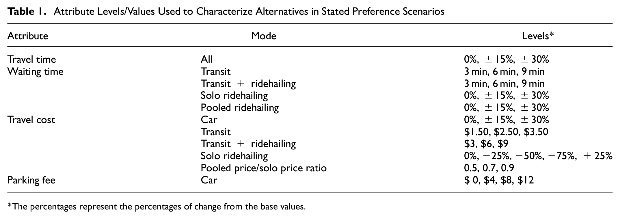
The percentages represent the percentages of change from the base values.

Data Collection

Because of the large number of alternatives and their associated attributes, we conducted a random sampling approach to reduce respondent burden. We used a fractional factorial experimental design to develop a balanced and orthogonal set of 9,000 choice scenarios including 6,000 choice scenarios with conventional vehicles in block sizes of four, and 3,000 choice scenarios with AVs in block sizes of two. These scenarios were then partitioned randomly into sets of six. We checked the balance and orthogonality of the resulting design and found that the main effects and two-way interactions were unconfounded. The “AlgDesign” R package was used to generate the fractional orthogonal designs.

Each respondent was presented with a total of six scenarios. In scenarios 1 to 4 they had to choose between conventional modes. Each respondent was presented with three or four alternatives per scenario and was asked to choose the preferred alternative for his/her daily commute trip from home to work. If someone reported driving as their current mode, they did not get a pure transit alternative, and if they were currently a transit commuter, they did not see a driving alternative. All ridehailing services were shown to each respondent, except that the transit plus ridehailing mode was displayed only if respondents’ commute trip took longer than 30 min by transit or included a transfer. The modes shown in scenarios 1 to 4 were the same in each case but with different attribute levels.

In scenarios 5 to 6, respondents chose between two modes only. One was their current commute mode (e.g., driving) and the second mode was randomly selected from the other four modes (e.g., solo ridehailing, pooled ridehailing, transit, transit plus ridehailing). One of these two modes was randomly displayed as autonomous (For the case of transit, its autonomous version would be transit plus autonomous ridehailing). The modes shown in scenario 6 were the same as those shown in scenario 5 but with different attribute levels.

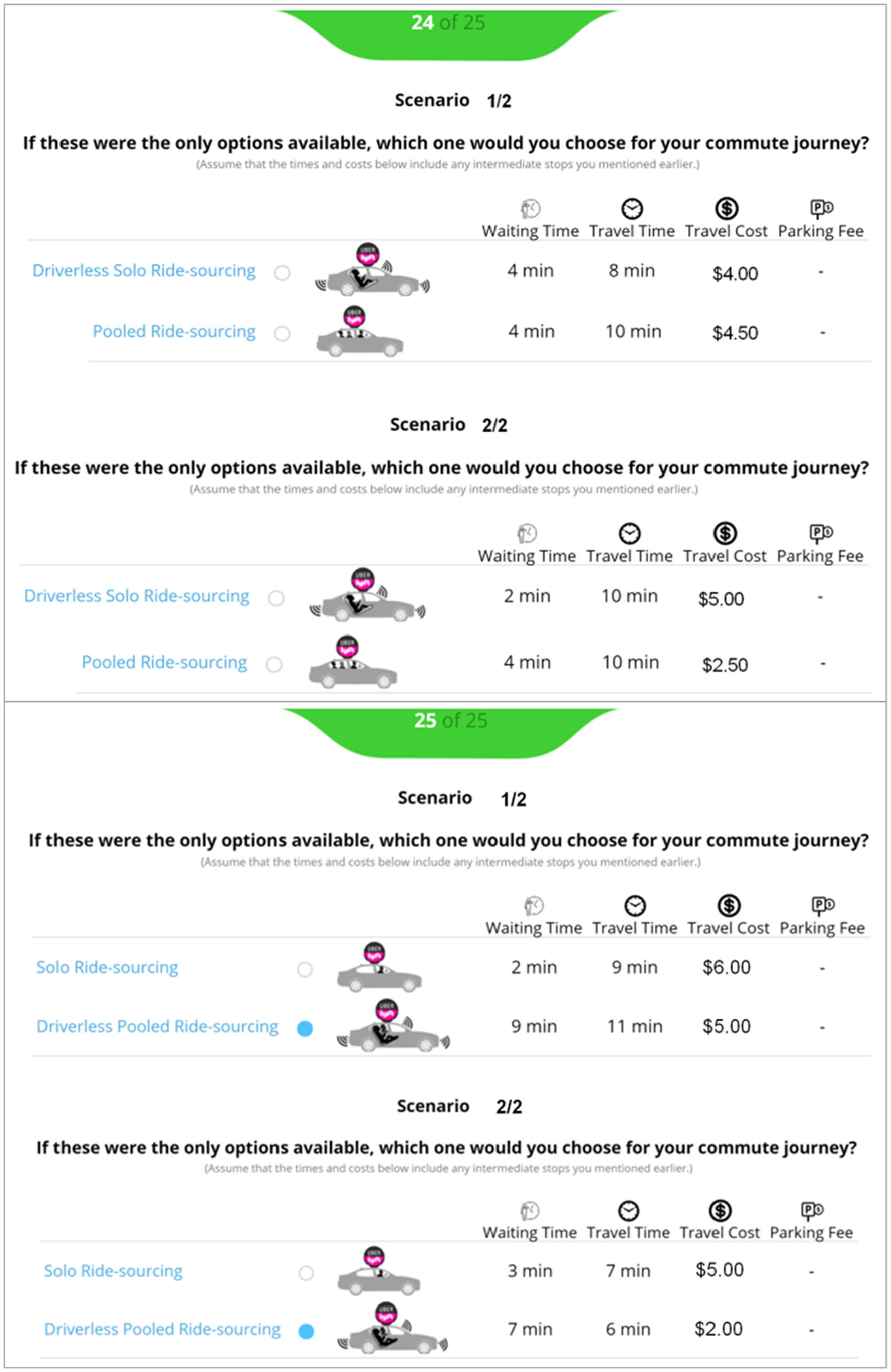
Figure 1 shows examples of two scenarios shown to different respondents in the final two choice scenarios (i.e., scenarios 5–6). For example, if a respondent reported “solo ridehailing” as his/her current commute mode, he/she was asked to choose either between “solo ridehailing” and autonomous version of a random mode, or between “autonomous solo ridehailing” and a random conventional mode. The random mode was randomly selected from the modes not currently used by the respondent (i.e., car, transit, transit plus ridehailing, and pooled ridehailing in this example).

Figure 1.

Examples of two sets of scenarios 5–6 shown to two different respondents.

The survey was implemented on Amazon Web Services (AWS) and was administered on Amazon’s Mechanical Turk (MTurk). MTurk is an online crowdsourcing marketplace that makes it easier for individuals and businesses to outsource their processes and jobs to a distributed workforce who can perform these tasks virtually. This could include anything from conducting simple data validation and research to more subjective tasks like survey participation, content moderation, and more. To have high-quality data, only the respondents with approval rates of 95% or higher on at least 100 previously completed MTurk tasks were qualified to take this survey. Although MTurk is widely used for data collection, the sample could be biased by MTurk respondents perhaps being younger, more educated, and more familiar with technology applications ( 29 – 33 ). The use of SP–RP analysis can help to reduce the impact of this bias on estimates, by bringing predicted market shares closer to actual market shares ( 25 , 28 ).

The survey was released in March 2019 on a nation-wide scale with a target sample size of 1,500 respondents, distributed proportionally to the population living in each of the four continental US time zones. This generated a total of 9,000 SP observations. To control data quality, we applied established quality-control techniques to identify and filter out data of low quality. In our experiment, low-quality data may result from several concerns. A particular concern with respondents being paid to complete a survey is that some may respond without giving adequate consideration to questions, or even randomly. To address these concerns, we conducted a consistency check across the sample to check for inconsistent responses. Also, we flagged the respondents with very long or very short survey completion times. Finally, after dropping respondents with current modes of walk or bike because of their low share, unemployed respondents, and those working from home, 6,753 observations were retained.

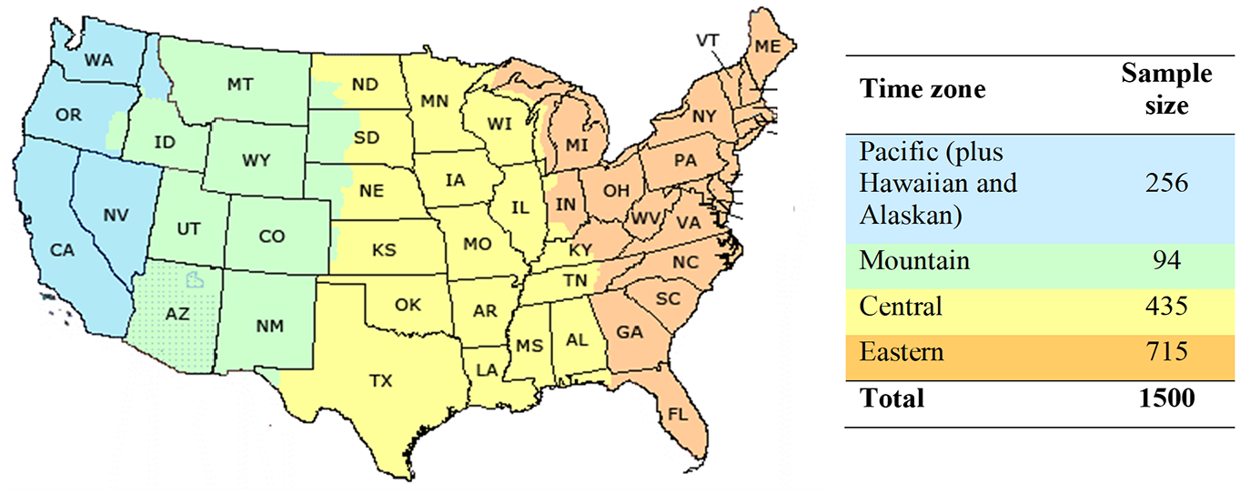
The geographic distribution of all the respondents who participated in the survey is displayed in Figure 2 , and Table 2 presents a summary of demographic statistics for the retained respondents in the final sample.

Figure 2.

Geographic distribution of the respondents around the US.

Table 2.

Summary of the Demographic Statistics of the Final Sample

Demographic variable	Category	Value (sample)	Value (US population)
Current commute travel mode	Car driver and car passenger	85.5%	85.6%
	Transit	9.0%	5.2%
	Bike	1.6%	0.6%
	Walk	2.2%	2.8%
	Solo ridesourcing	1.4%	NA
	Pooled ridesourcing	0.3%	NA
	Other	NA	5.8%
Mean travel time	Car	20.6 min	26.9 min
Mean travel time	Transit	54.0 min	51.0 min
Gender	Female	46.5%	49.9%
Gender	Male	53.5%	50.1%
Age	18–24	7.7%	9.5%
	25–34	42.6%	13.8%
	35–44	25.6%	12.6%
	45–54	15.5%	13.0%
	55–64	7.8%	12.9%
	65 or more	0.8%	15.6%
Education	Less than high school	0.4%	NA
	High school graduate	7.3%	NA
	BSc and higher	61.0%	32.0%
	Graduate and higher	16.0%	12.3%
Job	Full-time	86.4%	66.3%
	Part-time	11.1%	33.7%
	Student	2.5%	NA
Median age		34.0	37.8
Median household annual income	Under $20,000	4.6%	15.5%
	$20,000 to $39,999	19.2%	18.3%
	$40,000 to $59,999	21.0%	15.9%
	$60,000 to $99,999	34.6%	22.5%
	$100,000 to $199,999	18.0%	20.9%
	$200,000 or more	2.6%	6.9%
Mean persons per household		2.7	2.6
Mean vehicles per household		2.6	2.0

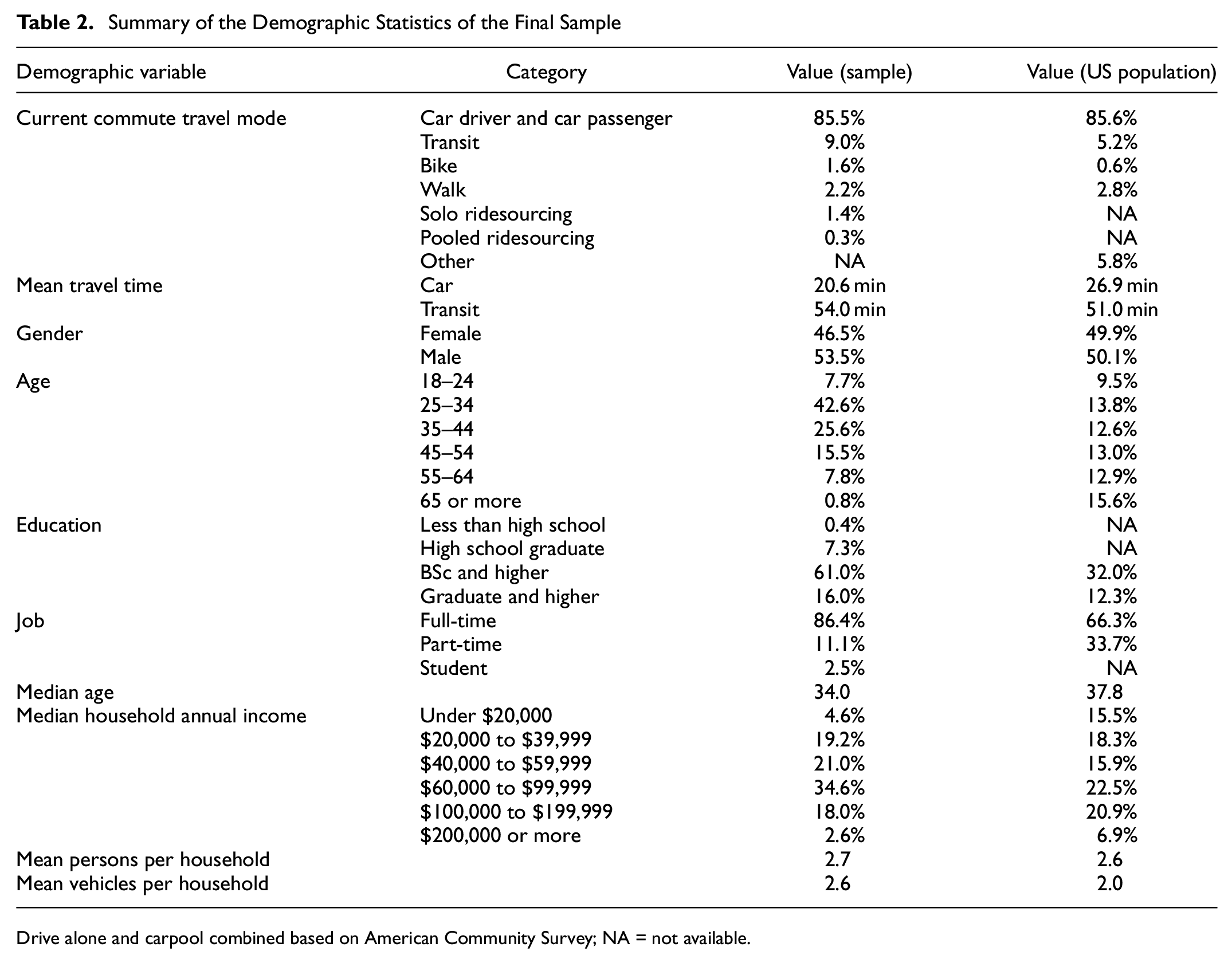
Drive alone and carpool combined based on American Community Survey; NA = not available.

Methods

A model developed based on pure SP data is prone to over- or under-estimating market shares because of hypothetical bias ( 25 ). The inclusion of RP data ensures that estimation is anchored to observed behavior, resulting in more realistic market share predictions.

Although the “nested logit trick” is the most common approach to pooling RP and SP data, it cannot account for correlations between repeated observations of the same respondent, such as in the six repeated choices made by each respondent in this study. More importantly, joint SP–RP estimation can cause a “state dependence” effect, defined as the impact of actual choice data (RP) on the individual’s stated choices (SP data) ( 34 ). Habit persistence or inertia in seeking an alternative may lead to a positive effect of state dependence, while a negative effect may result from the desire for variety or from latent dissatisfaction associated with the current alternative ( 34 ).

Most SP–RP studies ignore state dependence and adopt fixed parameters in pooling SP–RP data. This study has accommodated such unobserved heterogeneity in the state dependence effect of the RP choice on SP choices based on the approach suggested by Bhat and Castelar ( 34 ): see section 19 of ( 25 ) for more detail.

To model the mode choice behavior of commuters, using the joint SP–RP data, a mixed logit (MXL) model was built that can account for an error structure between alternatives including unobserved preference heterogeneity, correlated choice sets, SP–RP scale difference, and state dependency.

The mixed logit model develops as the vector form of the individual-specific parameter, β_i. We begin with the basic form of the MXL model, with alternative-specific constants, α_ji, and attributes, x_ji, for individuals i in choice setting t and a choice set comprising several alternatives including the qth and the jth:

β_{ki} = β_{k} + σ_{k} * ν_{ik};

(1)

and

α_{ji} = α_{j} + σ_{j} * ν_{ji}

(2)

where

β_k is the population mean;

v_ik is the individual-specific heterogeneity, with mean 0 and standard deviation 1;

σ_k is the standard deviation of the distribution of β_iks around β_k; and

α_ji represents the choice-specific constants.

The elements of β_i are randomly distributed across individuals with fixed means. The v_jkis are the source of the heterogeneity as individual and choice-specific unobserved random terms.

An additional layer of individual heterogeneity can be applied to the model in the form of error components capturing alternatives-related influences. This is done by creating a set of independent individual terms that can be applied to the utility functions. This system allows us to create what is a model of random effects and, moreover, a very general type of alternative nesting. Let independent individual terms be e_in (n = 1, . . ., N), normally distributed with mean 0 and standard deviation 1 (i.e., N[0,1]), and θ_n be the scale parameter (standard deviation) associated with these effects. Then, each utility function could be written as

U_{ijt} = α_{ji} + β_{j} X_{jit} + (any of {θ_{1}}_{i 1}, {θ_{2}}_{i 2}, \dots ., {θ_{N}}_{iN})

(3)

Assume a structure in a model with four utility functions as follows:

U_{i 1 t} = V_{i 1 t} + {θ_{1}}_{i 1} + θ_{2} e_{i 2}

(4)

U_{i 2 t} = V_{i 2 t} + θ_{2} e_{i 2}

(5)

U_{i 3 t} = V_{i 3 t} + {θ_{1}}_{i 1} + θ_{3} e_{i 3}

(6)

U_{i 4 t} = V_{i 4 t} + θ_{4} e_{i 4}

(7)

Therefore, there is a correlation between U_i_1t and U_i₂t and between U_i_1t and U_i_3t, while U_i_4t has its own uncorrelated effect. The simplest way to allow different structures is to use binary variables, d_jn = 1, if the random term e_n occurs in utility function j and 0 otherwise.

Some specific characteristics of the model of interest in joint estimation with multiple datasets (i.e., SP and RP datasets) include the possibility of “state (reference) dependence” created in the SP data as a derivative of a market context of RP data; and the differences in the scale parameters for the SP data compared with the RP data. State dependence is defined by Bhat and Castelar ( 34 ) as

φ_{q} (1 - δ_{qt, RP})

(8)

where δ_qt, _RP = 1 if an RP observation, 0 otherwise, and φ_q is the state dependency parameter which can be fixed or random. For each SP alternative, this variable enters the utility function, with the ability to select a generic specification.

The scale parameter for the SP dataset relative to the RP dataset is obtained through the introduction of a set of alternative-specific constants (ASCs) that have a zero mean and free variance in the SP data while the scale for the RP dataset is normalized to 1.0 ( 35 ). The scale parameter is calculated using

λ_{qt} = [(1 - δ_{qt, RP}) λ] + δ_{qt, RP}

(9)

According to Equation 9 , the δ_qt, _RP was defined above and λ is inversely proportional to the estimated standard deviation of the ASC of an alternative, according to the EV1 distribution,

λ = \frac{π}{\sqrt{6} * Standard Deviation of ASC}

Then a model with error components for each alternative is identified. Unlike other specifications ( 36 ) that use the results to identify the scale factors in the disturbances of the utility functions, the logic is not used to identify the parameters on the attributes; and in the conditional distribution we are looking at here, the error components act as attributes, not as disturbances. Also, the θ parameters are estimated as if they are weights on attributes, not scales on disturbances. The parameters are identified in the same way that the βs are identified on the attributes.

As the error components are not observed, their scale is not identified. Therefore, the parameter on the error component is (δ_nσ_n) in which σ_n is the standard deviation. Given that the θ carries the magnitude and sign of the parameter on the component, the scale is normalized to 1 for estimation purposes as it is unidentified. Also, since the sign of δ_m is not identified, we normalize the sign to plus, and estimate |δ_m| with the sign and the value of σ_m normalized for identification purposes.

Results

Model Results

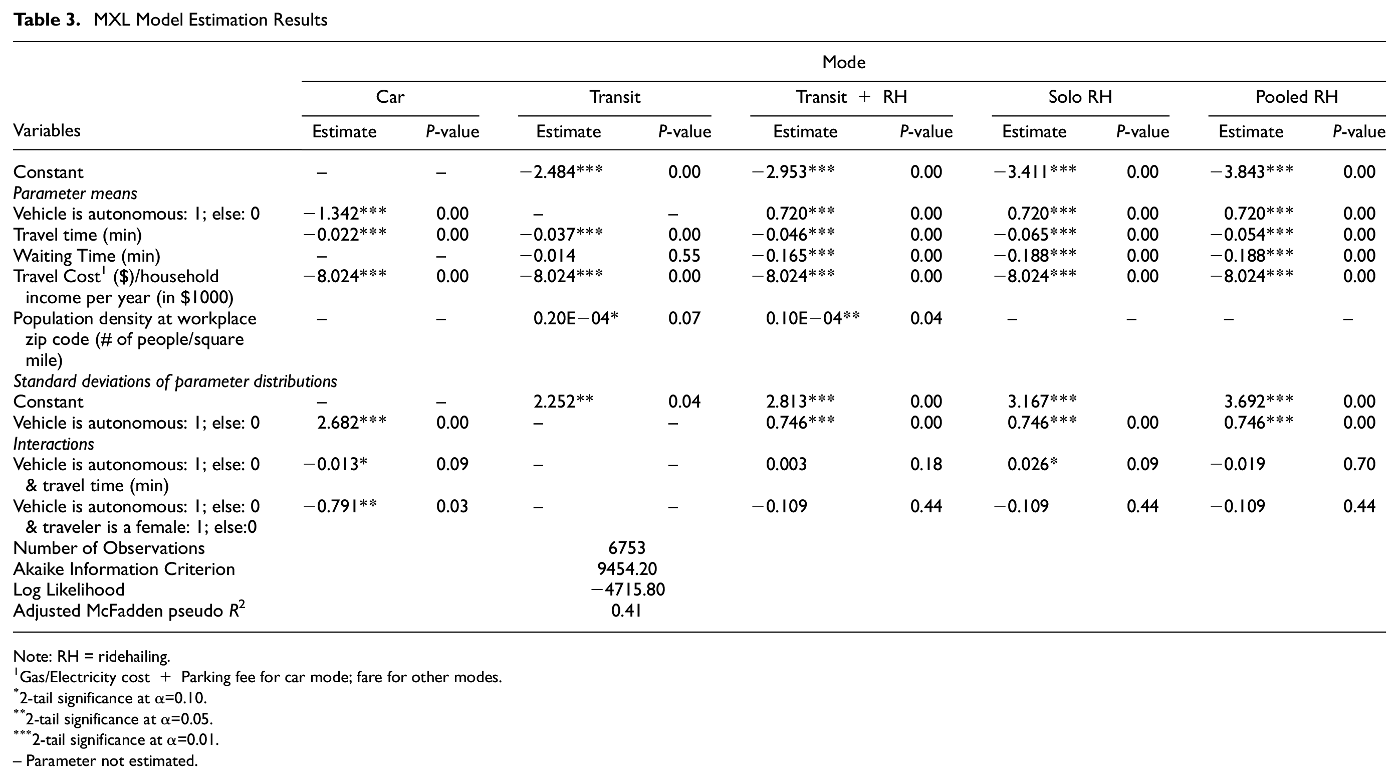
The results of the mixed logit model estimated in BIOGEME 3.2.5 are presented in Table 3 . To find the possible factors affecting the mode choice behavior of individuals, the pairwise Spearman correlation test was conducted, and the variables with acceptable levels of significance (α = 0.01, α = 0.05, and α = 0.10) were identified for the modeling process.

Table 3.

MXL Model Estimation Results

Variables	Mode
	Car		Transit		Transit + RH		Solo RH		Pooled RH
	Estimate	P-value	Estimate	P-value	Estimate	P-value	Estimate	P-value	Estimate	P-value
Constant	–	–	−2.484***	0.00	−2.953***	0.00	−3.411***	0.00	−3.843***	0.00
Parameter means
Vehicle is autonomous: 1; else: 0	−1.342***	0.00	–	–	0.720***	0.00	0.720***	0.00	0.720***	0.00
Travel time (min)	−0.022***	0.00	−0.037***	0.00	−0.046***	0.00	−0.065***	0.00	−0.054***	0.00
Waiting Time (min)	–	–	−0.014	0.55	−0.165***	0.00	−0.188***	0.00	−0.188***	0.00
Travel Cost¹ ($)/household income per year (in $1000)	−8.024***	0.00	−8.024***	0.00	−8.024***	0.00	−8.024***	0.00	−8.024***	0.00
Population density at workplace zip code (# of people/square mile)	–	–	0.20E−04*	0.07	0.10E−04**	0.04	–	–	–	–
Standard deviations of parameter distributions
Constant	–	–	2.252**	0.04	2.813***	0.00	3.167***		3.692***	0.00
Vehicle is autonomous: 1; else: 0	2.682***	0.00	–	–	0.746***	0.00	0.746***	0.00	0.746***	0.00
Interactions
Vehicle is autonomous: 1; else: 0 & travel time (min)	−0.013*	0.09	–	–	0.003	0.18	0.026*	0.09	−0.019	0.70
Vehicle is autonomous: 1; else: 0 & traveler is a female: 1; else:0	−0.791**	0.03	–	–	−0.109	0.44	−0.109	0.44	−0.109	0.44
Number of Observations	6753
Akaike Information Criterion	9454.20
Log Likelihood	−4715.80
Adjusted McFadden pseudo R²	0.41

Note: RH = ridehailing.

Gas/Electricity cost + Parking fee for car mode; fare for other modes.

2-tail significance at α=0.10.

2-tail significance at α=0.05.

***

2-tail significance at α=0.01.– Parameter not estimated.

Several models were developed with different attributes including socio-economic variables, population density of home and workplace location, and interactions of different income bins and travel cost.

Random parameters in normal distributions have been employed for ASCs and for the automation attribute. Automation has been adopted as an attribute for car and for solo and pooled ridehailing modes including the ridehailing used for the first-/last-mile connection in transit plus ridehailing mode. The coefficients of automation were also assumed to be the same for all ridehailing modes (solo, pooled, and transit plus ridehailing). In addition, the coefficients of waiting time were assumed to be the same for solo and pooled ridehailing. Travel cost was divided by the midpoint of the income category reported by the respondent and was implemented as a generic variable with the same coefficient in all the utility functions.

All travel time parameters were found significant with negative signs for coefficients, which is consistent with intuition. The coefficients for waiting time also have negative signs, but waiting time is statistically insignificant for the transit alternative.

The results also showed that the population density at the respondent’s workplace location has a positive impact on choosing transit and transit plus ridehailing. This might be related to the higher level of transit accessibility in dense areas with a lot of parking and congestion issues, which makes non-car modes often more favorable in these settings.

Furthermore, several covariates were investigated as possible sources of heterogeneity around the means of the random parameter estimates. In effect, interacting random parameters with other covariates decomposes the heterogeneity observed within the random parameter, offering an explanation as to why that heterogeneity may exist ( 25 ). The random parameters for which a covariate was found to partly explain the variation in marginal utilities included car automation, car travel time, and travel cost for all modes. The statistically significant and negative parameter for the interaction term of the random parameter, car automation, and the covariate, gender of a traveler, suggests that female travelers are generally less willing to ride in AVs. Other variables including age and car ownership were also interacted with automation but were found to be statistically insignificant as sources of heterogeneity in our sample. Also, the interaction of the random parameter, car automation, with travel time attribute indicates that automation might lead to an increase in the average value of travel time savings (VTTS) for private cars and a decrease in the VTTS for solo ridehailing. The VTTS values implied by our results for each mode are reported in Table 4 , along with 95% confidence limits.

Table 4.

Value of Travel Time Savings (VTTS)

Travel mode	VTTS ($/h)
Travel mode	Conventional	Autonomous
Car	11.1 [8.2, 14.0]*	17.7 [6.1, 29.4]
Transit	17.8 [14.1, 21.6]	na
Transit + ridehailing	22.4 [20.1, 24.7]	21 [15.4, 26.6]
Solo ridehailing	31.3 [26.6, 36.0]	18.4 [15.2, 21.6]
Pooled ridehailing	26.7 [22.4, 31.0]	35.7 [25.6, 45.8]

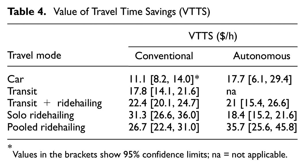
Values in the brackets show 95% confidence limits; na = not applicable.

The VTTS for autonomous ridehailing was found to be higher than that of a conventional car. This result is counterintuitive, as in theory it is believed that being freed from the need to drive would decrease the VTTS. However, a few other studies also found the same results ( 14 , 37 , 38 ), suggesting that since AVs are not yet commercially available, people are not familiar/comfortable enough with autonomous cars and their stated choices today may not reflect choices they make in the future. The VTTS for autonomous pooled ridehailing is higher than that of autonomous solo ridehailing. This may reflect concerns with sharing a ride in an autonomous car with strangers when no driver is present. Since we do not have the data necessary to test these hypotheses, we leave it to other studies in the future.

Sensitivity Analysis

After building the choice model, a sensitivity analysis was conducted to measure the impact of automation on the behavior of transit commuters. Automation and electric propulsion technologies are predicted to allow a substantial decrease in prices for all modes ( 39 ). Furthermore, automation is expected to affect the perceived cost of travel by drivers ( 37 , 38 , 40 ), and it is expected to reduce the travel time and waiting time by optimizing the efficiency of mobility services ( 19 , 41 , 42 ).

Therefore, this section explores the potential mode share effects of a decrease in the price, travel time, and waiting time of ridehailing in two scenarios. The ranges of decreases in the attributes are consistent with ranges of variable values covered in the experimental design in Table 1 .

Scenario 1

In this scenario, it is assumed that none of the modes are autonomous, and the effects of varying price, travel time, and waiting time of conventional ridehailing modes on the attraction of transit commuters are simulated. The baseline for this analysis is status quo; that is, when all modes are conventional, and they keep their current attribute values.

A. Price

As shown in Figure 3 , the price of conventional ridehailing modes has been decreased by 10% increments (X axis) and the market share for each of the three conventional ridehailing modes (i.e., solo, pooled, and first/last mile) along with the transit market share has been calculated (Y axis).

B. Travel time and waiting time

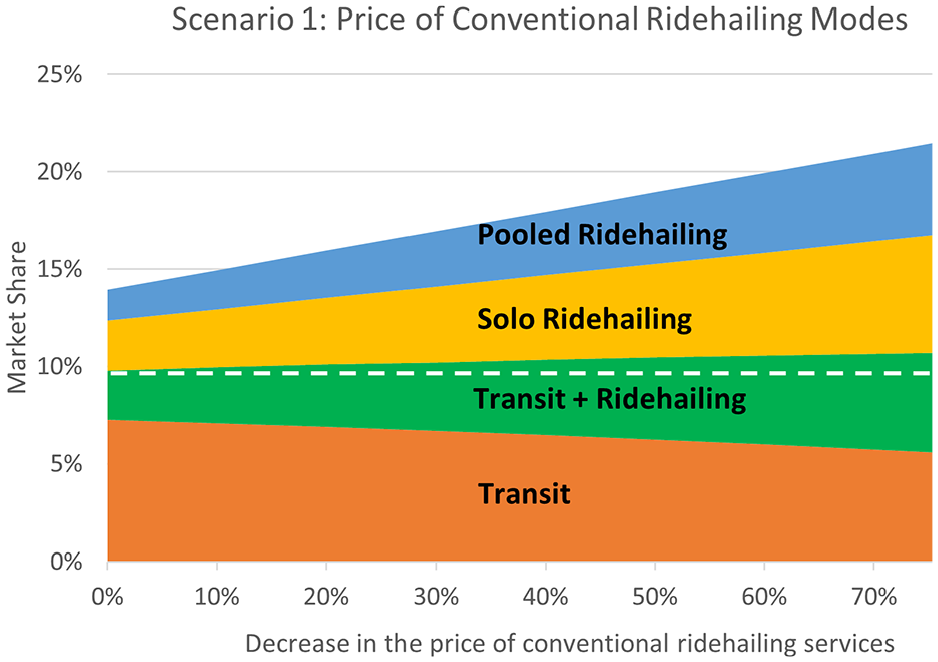
Figures 4 and 5 show how the market shares of the three conventional ridehailing modes (i.e., solo, pooled, and first/last mile) and transit depend on the ridehailing travel time and waiting time, respectively.

Figure 3.

Change in the market share of transit and ridehailing modes as a result of decreased price of conventional ridehailing services.

Figure 4.

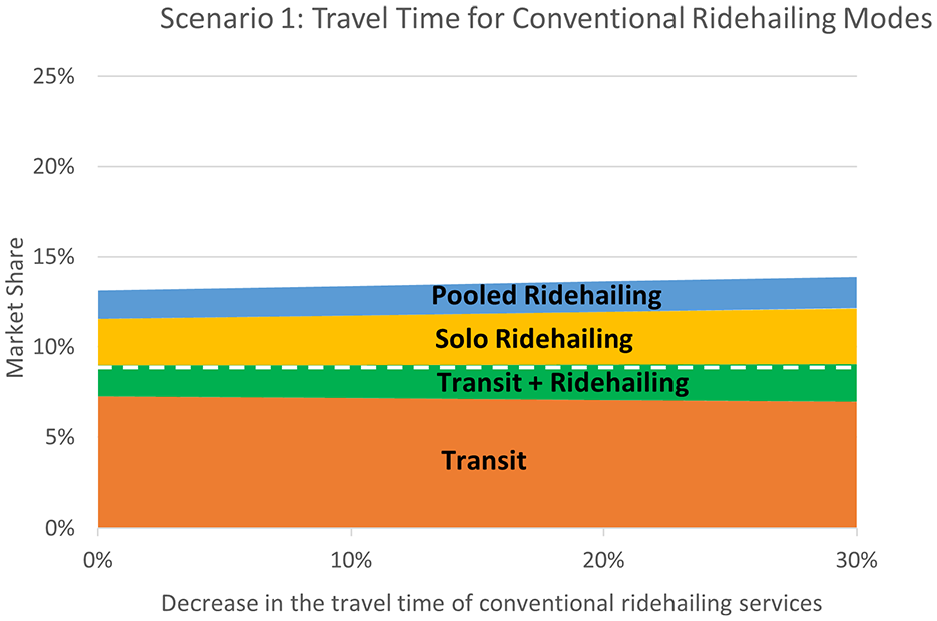
Change in the market share of transit and ridehailing modes as a result of decreased travel time for conventional ridehailing services.

Figure 5.

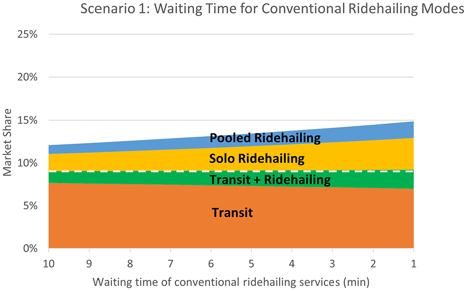
Change in the market share of transit and ridehailing modes as a result of decreased waiting time for conventional ridehailing services.

Figure 3 , which involves conventional modes, shows that as the transit market share is decreased, the market shares of ridehailing services increase. Among ridehailing modes, the market shares of solo and pooled ridehailing grow faster than that of ridehailing as a first-/last-mile connection to transit. It is also shown that transit-only market share decreases, but overall transit share, including transit-only riders and those who use ridehailing for first-/last-mile connection to transit, remains mostly constant, or slightly increases (compared with the horizontal white dashed line).

Figures 4 and 5 , which involve conventional modes, indicate that a decrease in the travel time and waiting time of conventional ridehailing services leads to a decrease in the market share of transit-only mode while the total market share for transit, including transit-only riders and those who use ridehailing for first-/last-mile connection to transit, remains mostly constant (indicated by the white dashed line).

Scenario 2

In this scenario, all modes are assumed to be autonomous, and again the effects of varying the price, travel time, and waiting time of autonomous ridehailing modes on the market share of transit commuters are simulated. The baseline for this analysis is when all modes are autonomous, but they keep their other attributes at current levels.

A. Price

As can be seen in Figure 6 , The price of autonomous ridehailing has been decreased by 10% in each step (X axis) and the market share for each of the three autonomous ridehailing modes (i.e., solo, pooled, and first/last mile) along with transit market share has been calculated (Y axis).

B. Travel time & Waiting time

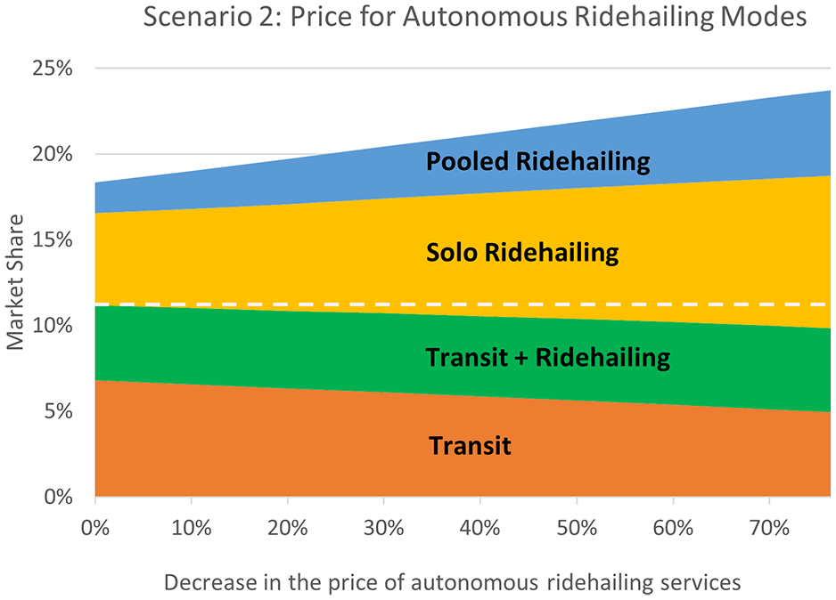
Figures 7 and 8 show how the market shares of the three autonomous ridehailing modes (i.e., solo, pooled, and first/last mile) and transit depend on the autonomous ridehailing travel time and waiting time, respectively.

Figure 6.

Change in the market share of transit and ridehailing modes as a result of decreased price of autonomous ridehailing services.

Figure 7.

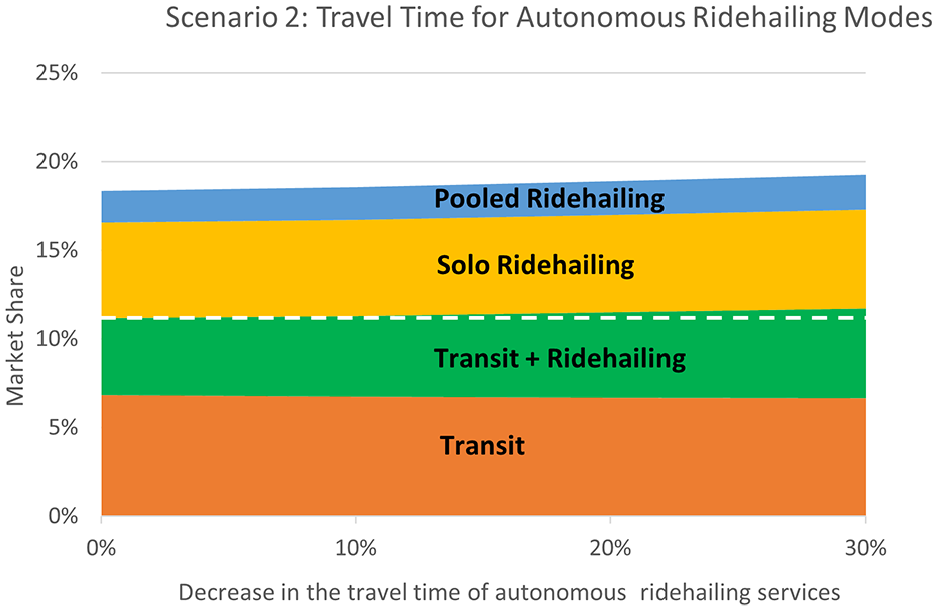
Change in the market share of transit and ridehailing modes as a result of decreased travel time for autonomous ridehailing services.

Figure 8.

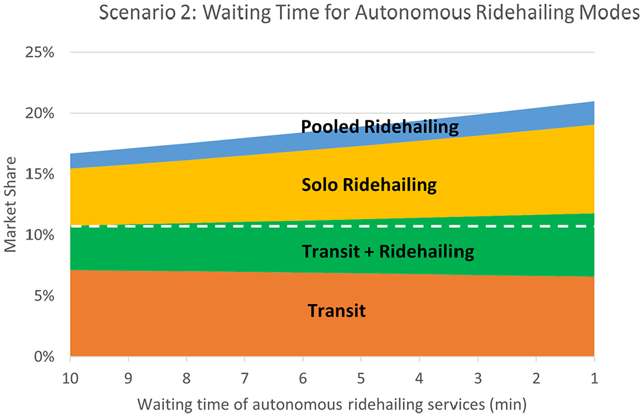
Change in the market share of transit and ridehailing modes as a result of decreased waiting time for autonomous ridehailing services.

In Figure 6 , which involves autonomous services, transit-only market share decreases, while the market share of transit plus ridehailing as first-/last-mile connection remains roughly constant. Therefore, overall transit share decreases slightly as indicated by the white dashed line.

In Figures 7 and 8 which involves autonomous services, reduction in travel time and waiting time has led to an increase in the market share of ridehailing services while the transit-only market share has dropped. However, the overall transit market share suggests an increase as indicated by the white dashed line.

Furthermore, comparing Figure 3 with Figure 6 reveals that a potential decrease in the price of ridehailing services caused by automation accelerates the trend of shifting from transit to solo ridehailing and transit plus ridehailing, while pooled ridehailing might not benefit too much from automation. This could be related to discomfort and privacy concerns caused by sharing a ride in an autonomous car with strangers when no driver is present ( 39 ). Although people generally prefer the privacy of their own car to the shared environment of a bus ride, many still consider it burdensome to share a car-sized vehicle with strangers ( 43 ).

According to Figure 3 , price reduction in conventional ridehailing services could keep the total transit market share constant by encouraging more transit users to use inexpensive ridehailing for the first-/last-mile connection to transit. In Figures 4 and 5 , like price reduction, travel time, and waiting time reduction in conventional ridehailing services could keep the total transit market share approximately constant.

As can be seen in Figure 6 , price reduction in autonomous ridehailing services could decrease the total transit market share by encouraging more transit users to shift to inexpensive autonomous ridehailing services, especially to solo ridehailing. In Figures 7 and 8 , unlike price reduction, travel time and waiting time reduction could maintain (yet increase) the total transit market share resulting from the increase in the usage of autonomous ridehailing as the first-/last-mile connection to transit.

Conclusions

In this study, we explored how the automation of ridehailing might affect transit market share. To understand how the changes in the commute mode shares depend on the characteristics of transportation modes, a survey was designed and distributed nationally that consisted of three parts: socio-economic questions, actual mode choice questions (i.e., RP data), and hypothetical mode choice questions (i.e., SP data). In the third part, various choice scenarios were developed that included five transportation modes: car, transit, transit plus ridehailing for the first/last mile, solo ridehailing, and pooled ridehailing. To model the behavior of commuters a mixed logit model was employed using joint SP–RP data, considering car as the reference mode.

The model results indicated that travel cost, waiting time, and travel time decrease utility of all modes, and higher population density at the work location increases the utility of transit and transit plus ridehailing modes. In addition to the choice model analysis, we also built and analyzed different scenarios, assuming different prices, waiting time, and travel times for ridehailing services as well as assuming the services being autonomous or conventional.

It was found that ridehailing per se might not be a significant competitor to transit, especially if it is integrated with transit as a first-/last-mile service. With conventional ridehailing services, the total transit mode share (transit-only riders plus those who use transit in connection with ridehailing for first/last mile) remains largely flat even if ridehailing fares decrease. On the other hand, if automation significantly reduces the price of ridehailing services, our analysis suggests a decline in total transit ridership and an increase in ridehailing, especially for solo ridehailing in commute trips. This could lead to major challenges with traffic congestion and emissions. Ridehailing services already face taxation and other regulations by cities, and additional policies may be needed in a future with autonomous ridehailing to offset the effects of automation-enabled labor cost reductions. The results also suggest that the better services by ridehailing companies to minimize travelers’ waiting time and travel time may not negatively affect the total transit market share, regardless of the service being conventional or autonomous. The results also imply that autonomous pooled ridehailing might not be as attractive to commuters as autonomous solo ridehailing, which could be an important insight for transportation network companies (TNCs).

In future studies, it will be interesting to include other modes such as walking and biking to figure out the shift between those and ridehailing services, as automation is introduced and/or prices change. Also, future studies could focus on the attitudes of individuals toward autonomous pooled ridehailing to gain insights about the reluctancy or willingness of people to the automation of this mode. Since the workplace population density was found to have a positive and statistically significant effect on choosing transit and transit plus ridehailing modes, it would be desirable to examine how other land use attributes such as employment density and land use diversity affect the choice between transit and ridehailing services, particularly given the future availability of AVs. Finally, we should note that the data for this study were collected a year before the COVID-19 pandemic hit the US, and so the data and market share estimates might not reflect current or near future attitudes toward ridehailing and/or transit services.

Footnotes

Declaration of Conflicting Interests

The author(s) declared no potential conflicts of interest with respect to the research, authorship, and/or publication of this article.

Funding

The author(s) disclosed receipt of the following financial support for the research, authorship, and/or publication of this article: This research was provided by Toyota Motor Engineering & Manufacturing North America Inc.

ORCID iDs

Andisheh Ranjbari

Ken Laberteaux

Don Mackenzie

References

MacKenzie

(2021). The Evolution, Usage and Trip Patterns of Taxis & Ridesourcing Services: Evidence from 2001, 2009 & 2017 US National Household Travel Survey. Transportation. https://doi.org/10.1007/s11116-021-10177-5.

Hall

J. D.

Palsson

Price

Is Uber a Substitute or Complement for Public Transit?

Journal of Urban Economics, Vol. 108, 2018, pp. 36–50.

Rayle

Dai

Chan

Cervero

Shaheen

Just a Better Taxi? A Survey-Based Comparison of Taxis, Transit, and Ridesourcing Services in San Francisco. Journal of Transport Policy, Vol. 45, 2016, pp. 168–178.

Greenwood

B. N.

Wattal

Show Me the Way to Go Home: An Empirical Investigation of Ride Sharing and Alcohol Related Motor Vehicle Homicide. Management Information Systems Quarterly, Vol. 41, No. 1, 2017, pp. 163–188.

Smith

B. W.

Managing Autonomous Transportation Demand. Santa Clara Law Review, Vol. 52, 2012, p. 1401.

Anderson

J. M.

Nidhi

Stanley

K. D.

Sorensen

Samaras

Oluwatola

O. A.

Autonomous Vehicle Technology: A Guide for Policymakers. RAND Corporation, Santa Monica, CA, 2016.

Gruel

Stanford

J. M.

Assessing the Long-Term Effects of Autonomous Vehicles: A Speculative Approach. Transportation Research Procedia, Vol. 13, 2016, pp. 18–29.

Wen

Chen

Y. X.

Nassir

Zhao

Transit-Oriented Autonomous Vehicle Operations with Integrated Demand-Supply Interaction. Transportation Research Part C: Emerging Technologies, Vol. 97, 2018, pp. 216–234.

Levin

M. W.

Boyles

S. D.

Effects of Autonomous Vehicle Ownership on Trip, Mode, and Route Choice. Transportation Research Record: Journal of the Transportation Research Board, 2015. 2493: 29–38.

10.

Liang

de Almeida Correia

G. H.

Van Arem

Optimizing the Service Area and Trip Selection of an Electric Automated Taxi System Used for the Last Mile of Train Trips. Transportation Research Part E: Logistics and Transportation Review, Vol. 93, 2016, pp. 115–129.

11.

Vakayil

Gruel

Samaranayake

Integrating Shared-Vehicle Mobility-On-Demand Systems with Public Transit. Technical Report17-05439. Transportation Research Board of the National Academies, Washington, D.C., 2017.

12.

Shen

Zhang

Zhao

Integrating Shared Autonomous Vehicle in Public Transportation System: A Supply-Side Simulation of the First-Mile Service in Singapore. Transportation Research Part A: Policy and Practice, Vol. 113, 2018, pp. 125–136.

13.

Lenz

Fraedrich

New Mobility Concepts and Autonomous Driving: The Potential for Change. In Autonomous Driving: Technical, Legal and Social Aspects ( Markus Maurer

Gerdes

Lenz

Winner

, eds.), Springer, Berlin Heidelberg, 2016, pp. 173–191. https://doi.org/10.1007/978-3-662-48847-8.

14.

Yap

M. D.

Correia

van Arem

Preferences of Travelers for Using Automated Vehicles as Last Mile Public Transport of Multimodal Train Trips. Transportation Research Part A: Policy and Practice, Vol. 94, 2016, pp. 1–16.

15.

Moorthy

De Kleine

Keoleian

Good

Lewis

Shared Autonomous Vehicles as a Sustainable Solution to the Last Mile Problem: A Case Study of Ann Arbor-Detroit Area. SAE International Journal of Passenger Cars-Electronic and Electrical Systems, Vol. 10, 2017, pp. 328–336.

16.

Pinto

H. K.

Hyland

M. F.

Mahmassani

H. S.

Verbas

I. Ö.

Joint Design of Multimodal Transit Networks and Shared Autonomous Mobility Fleets. Transportation Research Part C: Emerging Technologies, Vol. 113, 2020, pp. 2–20.

17.

Alemi

Rodier

Simulation of Ridesourcing Using Agent-Based Demand and Supply Models Regional: Potential Market Demand for First Mile Transit Travel and Reduction in Vehicle Miles Traveled in the San Francisco Bay Area. No. 18-05283. National Center for Sustainable Transportation, UC Davis, 2018.

18.

Fagnant

D. J.

Kockelman

K. M.

The Travel and Environmental Implications of Shared Autonomous Vehicles, Using Agent-Based Model Scenarios. Transportation Research Part C: Emerging Technologies. 40: 1–13.

19.

Fagnant

D. J.

Kockelman

K. M.

Bansal

Operations of Shared Autonomous Vehicle Fleet for Austin, Texas, Market. Transportation Research Record: Journal of the Transportation Research Board, 2015. 2536: 98–106.

20.

Marczuk

K. A.

Hong

H. S. S.

Azevedo

C. M. L.

Adnan

Pendleton

S. D.

Frazzoli

, et al. Autonomous Mobility on Demand in Simmobility: Case Study of the Central Business District in Singapore. In: Proc., IEEE 7th International Conference on Cybernetics and Intelligent Systems (CIS) and IEEE Conference on Robotics, Automation and Mechatronics (RAM), Siem Reap, Cambodia, July 15–17, 2015, IEEE, pp. 167–172.

21.

Martinez

L. M.

Correia

G. H.

Viegas

J. M.

An Agent-Based Simulation Model to Assess the Impacts of Introducing a Shared-Taxi System: An Application to Lisbon (Portugal). Journal of Advanced Transportation, Vol. 49, 2015, pp. 475–495.

22.

Kloostra

Roorda

M. J.

Fully Autonomous Vehicles: Analyzing Transportation Network Performance and Operating Scenarios in the Greater Toronto Area, Canada. Technical Report 17-00418. Transportation Research Board of the National Academies, Washington, D.C., 2017.

23.

Zhu

Kornhauser

A. L.

The Interplay between Fleet Size, Level-of-Service and Empty Vehicle Repositioning Strategies in Large-Scale, Shared-Ride Autonomous Taxi Mobility-On-Demand Scenarios. Technical Report 17-05960. Transportation Research Board of the National Academies, Washington, D.C., 2017.

24.

Swait

Louviere

Williams

A Sequential Approach to Exploiting the Combined Strengths of SP and RP Data: Application to Freight Shipper Choice. Transportation, Vol. 21, 1994, pp. 135–152.

25.

Hensher

D. A.

Rose

J. M.

Greene

W. H.

Applied Choice Analysis: A Primer. Cambridge University Press, New York, 2015.

26.

Freeman

A. M.

The Measurement of Environmental and Resource Values. Resources for the Future Press, Baltimore, 1993.

27.

Greene

W. G.

The HEV Model: A Note. Department of Economics, Stern School of Business, New York University, 1997.

28.

Louviere

J. J.

Hensher

D. A.

Swait

Stated Choice Methods: Analysis and Applications in Marketing. Transportation and Environmental Valuation, Cambridge University Press, Cambridge, 2000.

29.

Keith

M. G.

Tay

Harms

P. D.

Systems Perspective of Amazon Mechanical Turk for Organizational Research: Review and Recommendations. Frontiers in Psychology, Vol. 8, 2017, Article 1359.

30.

BouMjahed

Mahmassani

H. S.

Wired at Birth: Childhood, Technology Engagement, and Travel Behavior. Transportation Research Record: Journal of the Transportation Research Board, 2018. 2672: 66–78.

31.

Ranjbari

Lewis

E. O.

Barber

MacKenzie

Defining Psychometric Variables Related to Use of Autonomous Vehicles. Transportation Research Record: Journal of the Transportation Research Board, 2019. 2673: 655–669.

32.

Zou

Khaloei

MacKenzie

Effects of Charging Infrastructure Characteristics on Electric Vehicle Preferences of New and Used Car Buyers in the United States. Transportation Research Record: Journal of the Transportation Research Board, 2020. 2674: 165–175.

33.

Misra

Gooze

Watkins

Asad

Le Dantec

C. A.

Crowdsourcing and Its Application to Transportation Data Collection and Management. Transportation Research Record: Journal of the Transportation Research Board, 2014. 2414: 1–8.

34.

Bhat

C. R.

Castelar

A Unified Mixed Logit Framework for Modeling Revealed and Stated Preferences: Formulation and Application to Congestion Pricing Analysis in the San Francisco Bay Area. Transportation Research Part B: Methodological, Vol. 36, 2002, pp. 577–669.

35.

Brownstone

Bunch

D. S.

Train

Joint Mixed Logit Models of Stated and Revealed Preferences for Alternative-Fuel Vehicles. Transportation Research Part B: Methodological, Vol. 34, No. 5, 2000, pp. 315–338.

36.

Ben-Akiva

McFadden

Train

Walker

Bhat

Bierlaire

Bolduc

BoerschSupan

Brownstone

Bunch

Daly

de Palma

Gopinath

Karlstrom

Munizaga

M. A.

Hybrid Choice Models: Progress and Challenges. Marketing Letters, Vol. 13, No. 3, 2002, pp. 163–175.

37.

Gao

Ranjbari

MacKenzie

Would Being Driven by Others Affect the Value of Travel Time? Ridehailing as an Analogy for Automated Vehicles. Transportation, Vol. 46, No. 6, 2019, pp. 2103–2116.

38.

De Looff

Correia

G. D. A.

van Cranenburgh

Snelder

van Arem

Potential Changes in Value of Travel Time as a Result of Vehicle Automation: A Case Study in the Netherlands. Presented at 97th Annual Meeting of the Transportation Research Board, Washington, D.C., 2018.

39.

Bösch

P. M.

Becker

Axhausen

K. W.

Cost-Based Analysis of Autonomous Mobility Services. Transport Policy, Vol. 64, 2018, pp. 76–91.

40.

Khaloei

Ranjbari

MacKenzie

Analyzing the Shift in Travel Modes’ Market Shares with the Deployment of Autonomous Vehicle Technology. Presented at 99th Annual Meeting of the Transportation Research Board, Washington, D.C., 2020.

41.

Zhong

Lee

E. E.

Nejad

Lee

Influence of CAV Clustering Strategies on Mixed Traffic Flow Characteristics: An Analysis of Vehicle Trajectory Data. Transportation Research Part C: Emerging Technologies, Vol. 115, 2020, p. 102611.

42.

Soteropoulos

Berger

Ciari

Impacts of Automated Vehicles on Travel Behavior and Land Use: An International Review of Modelling Studies. Transport Reviews, Vol. 39, No. 1, 2019, pp. 29–49.

43.

Schmid

Schmutz

Axhausen

K. W.

Explaining Mode Choice, Taste Heterogeneity and Cost Sensitivity in a Post-Car World. Presented at the 95th Annual Meeting of the Transportation Research Board, Washington, D.C., 2016.