Daily Traffic Count Imputation for Bicycle and Pedestrian Traffic: Comparing Existing Methods with Machine Learning Approaches

Abstract

Monitoring nonmotorized traffic is becoming increasingly common practice at local and state departments of transportation. These travel activity data are necessary to monitor the system and track progress toward active transportation policy and program goals. A common problem is that permanent count site data are often missing, making those sites less useful. Being able to accurately estimate those missing data records functionally increases the amount of data available to use by themselves as metrics for monitoring traffic but also makes available more data for factoring short-term sites. Using nonmotorized traffic counts from several cities in Oregon, this research compared the ability of day-of-year (DOY) factors, a statistical model, and machine learning algorithms to accurately impute daily traffic records for annual traffic estimation. Based on exhaustive cross-validation experiments using data not missing at random scenarios, this research concluded that random forest and DOY factor approaches could be used to impute daily counts for nonmotorized traffic but each approach comes with tradeoffs. Though for many missing data scenarios random forest performed best, this method is complicated to estimate and apply. DOY factor-based methods are simpler to create and apply, and though more accurate in scenarios with significant amounts of missing data, they were less flexible given the need for data from neighboring count sites. Negative binomial regression was also found to work well in scenarios with moderate to low amounts of missing data. This work can inform nonmotorized traffic count programs needing vetted solutions for traffic data imputation.

Monitoring bicycle and pedestrian traffic is becoming increasingly common practice at local and state departments of transportation (DOTs). These travel activity data are necessary to monitor the system and track progress toward active transportation policy and program goals. Reliable traffic count data help practitioners measure travel activity before and after new infrastructure are built, as well as for use in safety analyses: these data can properly account for exposure and isolate the effect of the treatment under evaluation. Proper monitoring requires a combination of permanent counters collecting data throughout the year to develop reliable seasonable adjustment factors, which are applied to short-term counts. These short-term counts are most useful when extrapolated to an annual average daily traffic (AADT) estimate using expansion factors derived from permanent count sites ( 1 ).

A common problem however is that permanent count site data are often missing, making the data from those sites less useful. Being able to accurately estimate or impute those missing data records would functionally increase the amount of data available to use by themselves as metrics for monitoring traffic as well as make available more data for expanding short-duration count sites. If an agency has a large number of permanent nonmotorized traffic counters with similar traffic patterns, then previously tested day-of-year (DOY) methods may be sufficient. However, if permanent count sites are few or they exhibit sufficiently divergent temporal patterns, more sophisticated statistical methods or machine learning methods are more appropriate. If a given permanent count site exhibits a unique temporal pattern and has a significant amount of missing data, imputation using machine learning may be the best option.

This paper documents parametric and nonparametric approaches in addition to more simplistic factoring methods of nonmotorized traffic data to demonstrate that reliable estimation of missing data records is achievable through imputation. This research examined the tradeoffs to each of the approaches in relation to accuracy, complexity, and practicality for different real-world situations faced by DOTs managing traffic count data. The work documented here concluded that no one method worked best in all missing data scenarios and the applied imputation approach should therefore be tailored to the missing data scenario. These methods were tested in detail following a review of traffic imputation methods, including a more in-depth dive into existing expansion factor and imputation methods for nonmotorized traffic data.

Literature Review

In the past, motorized vehicle traffic count data imputation was relatively widespread with Albright documenting at least 23 states using some procedure for imputation on their permanent counter devices ( 2 ). Imputation is often necessary because of the common occurrence of missing data in automatic traffic recorders or ITS data collection devices ( 3 ). Though widespread, data imputation became a questionable practice as public agencies neglected to flag data that were imputed from those that were actually observed, leading to a small crisis of confidence in the traffic count data. In the early 1990s, the American Society for Testing and Materials and the Association of State Highway Transportation Officials adopted a base data integrity principle that highlighted the significance of raw traffic measurements being retained without modification or adjustment. Further, the principle of truth in data directs highway agencies to clearly document any procedures applied in imputation ( 3 ). As ITS systems that collect traffic volume data have expanded, imputation methods are needed both to fill in missing data and to forecast traffic conditions on a short-term basis for operational needs. Missing data for these systems have been reported to be as much as 15% ( 4 ) and 14% ( 5 ). Most of the recent literature documents statistically principled techniques for data imputation and seems to shed the simplistic methods of the past, using them as baseline methods for comparison. Comparison across studies is hard because some authors report estimation results for hourly counts whereas others look at monthly or annual estimation quantities.

Traffic count imputation uses three broad categories of methods, including historical and factor-based, time series analysis, and machine learning. Historical or factor-based methods use historical observations of traffic at a given location to fill in missing data or develop factors using traditional factoring approaches to estimate missing data. Moving average techniques use varying levels of sophistication to employ larger sets of observations to inform imputed values for missing data. Machine learning approaches may utilize a variety of algorithmic techniques including tree-based, ensemble, and neural networks.

In a survey of state DOT monitoring programs from 1990, it was found that at least seven states used simplistic procedures for imputing missing vehicle traffic-count records. For instance, it was found that South Dakota DOT would use the previous 3 years of counts for the same period needed for imputation to inform their missing values, whereas Delaware DOT would look at the same period during the previous and following month to inform their missing data estimate ( 2 ). Some of these approaches were reviewed ( 6 ) and found that for estimating hourly traffic counts, these simplistic, historical approaches resulted in more error compared with a relatively more sophisticated moving average approach. Alternatively, Turner and Park tested historical factor approaches on a number of scenarios for which data were missing at random and also not at random, finding that even when missing up to 8 months of data, error was low at less than 5% ( 7 ).

A time series is a chronological series of data on a given variable, in this case traffic count data collected on a 5 min, hourly, or daily basis. Time series data are analyzed in the hope of finding a historical pattern, for use in forecasting unknown, typically future values. Time series modeling is based on the assumption that previous trends offer information to predict future values ( 8 ). Numerous techniques exist for modeling univariate time series analysis, such as Holt–Winters, exponential smoothing and Box–Jenkins. Exponential smoothing should not be applied to data with seasonal variation; instead, the Holt–Winters procedure should be applied. The Box–Jenkins procedure is a common tool for time series analysis and is more commonly referred to as the autoregressive integrated moving average (ARIMA) model. Autoregressive and moving average components are considered in these models, thus the designation “integrated” model since the stationary model that is estimated to the differenced data has to be summed or integrated to provide a model for the nonstationary data ( 9 ). It has been noted that the ARIMA model with exponential smoothing and Holt–Winters approaches are equivalent ( 10 ). Sharma and colleagues used an ARIMA model and found it worked better for predicting hourly volumes compared with a time delay neural network, and the factor approach ( 11 ). Various versions of the moving average procedure have been used in traffic imputation since at least the 1990s when it was employed by London’s Department of Transportation ( 12 ). Zhong et al. found the moving average approach employed by London DOT performed better than the historic and factor-based approaches of some state DOTs ( 6 ).

Traffic imputation for bicycle and pedestrian traffic has been researched less than motorized traffic, though a significant body of work has been crafted looking at the question of short-duration traffic expansion methodologies. Traffic expansion factors are used to expand a short-duration traffic count, typically a period of 1 to 7 days, to be more representative of the annual traffic volume. This approach uses relatively simplistic multiplicative factors or ratios based on observed temporal conditions at permanent traffic count locations ( 13 , 14 ). Though the expansion of short-duration counts to an annual average volume can be thought of as a data imputation problem in which missing data are very high, strictly speaking imputation is not the problem most of these researchers are trying to solve. Because of this, the research previously done on expansion factor methods is not performed in a way that provides actionable information for practitioners using these methods for imputation ( 15 – 21 ). That being said, factoring has shown itself to be an important method for expanding short-duration counts. Of all the factoring methods explored in the literature there is growing consensus that the DOY method is best at minimizing annual traffic estimation ( 15 ). Nordback et al. reviewed past research on expansion factors, concluding that the DOY factor disaggregated by weather conditions outperforms traditional factors. Multiple papers investigating DOY factor approaches show that for expanding short-duration counts using the DOY method, mean absolute error is 23% ( 16 ) 23% ( 17 ), 20% ( 18 ), 17.5%, ( 19 ) 12% ( 20 ), 10% ( 21 ) in the best circumstances. These mean absolute error measures are subject to multiple conditions including the number of sites included in the tests, the independence of factor development data to testing data, and the process by which simulated short-duration count sites are matched to reference sites. Nevertheless they provide a decent benchmark with which to compare the results of the methods evaluated in this research. Results from past research do not typically test short-duration counts of more than 4 weeks and therefore leave questions regarding the application of the DOY method to longer periods of missing data.

Another limitation of the DOY factor approach is the need to match short-term sites with a single or a group of reference sites. This process introduces unknown error when applying factors if short-duration sites are not properly matched to a reference site or group or if insufficient sites exist in the expansion group ( 15 ). Beitel et al. enlists the DOY method for a data imputation problem to test the accuracy of imputation using DOY expansion factors ( 22 ). The authors propose a method for matching sites based on a correlation coefficient of 0.75 for sites where the annual average daily bicycle traffic is 250 bicycles per day or more. This research illustrated the effectiveness of the DOY factoring approach for data imputation when traffic count sites can be matched with other permanent sites. This approach however, requires enough data and counters to match the traffic count site to a reference site or group with similar DOY factors, which is not always possible. If conditions can be met for this method, error appears to be low, though in this research Beitel et al. did not examine the ability of the method to impute pedestrian counts ( 22 ). Since the DOY method works best when used to expand short-duration counts and has been used in research investigating a missing data problem, this method served as a baseline for comparing the methods proposed in this research, with more discussion below.

Other studies have investigated solutions for missing bicycle traffic data. El Esawey tested a Monte Carlo Markov Chain (MCMC) multiple imputation model to impute missing data including data missing completely at random (MCR) and data not missing at random (NMR) ( 18 ). The idea behind this approach is to take advantage of information from historical data from the count station and patterns in data from neighboring stations to develop an estimate of missing data. The tests found that the MCR tests were better than the NMR but only tested missing data scenarios of up to 4 months. The work also found the MCMC was significantly better than the baseline method of using monthly factors. In the NMR data scenarios, the maximum error for 2, 3, and 4 months of missing data was 10%, 13%, and 19% respectively using the MCMC method. El Esawey investigated the spatiotemporal relationships between permanent bicycle count stations to establish the use of neighboring count sites to impute missing data at a site of interest ( 23 ). The reported absolute percent error was 19.5% when sites’ daily traffic patterns met an arbitrary 0.6 Pearson correlation threshold, whereas the error was further reduced by increasing the correlation threshold to 0.7 and 0.8 with absolute percent errors of 17.1% and 14.8% respectively ( 23 ). The author notes that when the threshold is increased the number of sites that qualify for imputation drop, meaning some sites would not have data imputed using this method.

Building on the knowledge that traffic at neighboring bicycle count sites correlate with each other, El Esawey et al. tested the use of a machine-learning-based technique called artificial neural networks (ANNs) to impute missing daily count data ( 24 ). Using information from neighboring locations in conjunction with historic data from the test site, the ANN method was reported to achieve a mean absolute percent error of 10% when 30% of the data were missing. The training data was partitioned based on a random selection of 70% of the available data making this research an investigation of an MCR data imputation problem. Additional research by El Esawey used an MCMC and multiple imputation aiming to utilize the spatial temporal relationships between counters and the daily bicycle traffic’s relationship to weather fluctuations ( 25 ). This approach aimed to test MCR missing data scenarios in which 10% to 90% of the data were missing, finding that mean absolute percent error was about 27% at 80% missing data and 12% at 10% missing data. Further analysis of the validation tests concluded that information from the neighboring sites alone was useful in creating imputed values with low error, though the author notes that including weather variables can increase the flexibility of this approach when applied in practice. El Esawey also tested statistical models using weather variables, days of the week, and variables for months of the year and compared them with historical average methods, finding that the statistical model resulted in a mean absolute percent error of 20% with the historical average model performing much worse. Roll and Proulx tested the use of simulated short-term counts in a negative binomial statistical model to estimate annual traffic ( 26 ). Though these methods were tested to determine their use as an expansion factor method replacement and not explicitly as an imputation experiment, the results show that the statistical model can produce annual estimates of traffic with as little as 2% error using as few as 6 weeks of data.

Machine learning has become a more common analytic approach when analyzing data sets containing complex interactions among covariates or features, and has been shown to compare well with traditional methods ( 27 , 28 ). Several kinds of machine learning algorithms exist and include supervised learning methods, for which a response variable is defined by the user, as well as unsupervised in which the algorithm determines patterns of importance. Machine learning tasks are typically categorized as either a classification or a regression problem. In classification problems the algorithm learns to predict a binary or categorical variable, whereas in a regression problem, the model predicts a continuous variable. This research employed supervised learning algorithms for a regression problem (traffic counts) using tree-based methods including conditional inference and recursive partitioning as well as ensemble methods including random forest. Mathematical details of these machine learning approaches are outside the scope of this paper but the summary descriptions of each approach tested in this research are offered in Methods and Data. In addition, a detailed example of a tree-based machine learning approach is explored in the next section.

The conditional inference tree model is a commonly used decision tree model that explains the variable in the independent variable by recursively splitting the data feature into more homogenous groups using a combination of predictors. At each node split, data are divided into two groups based on a threshold value of one of the predictors with the aim of reducing the variance measured after the split compared with the variable before the split ( 29 ). This process is repeated until a specified criterion is met that maximizes predictive performance while executing the fewest number of splits. Conditional inference decision trees are implemented using Hothorn et al.’s statistical inference framework and represent an improvement over previous methods by solving two key problems ( 30 ). The first issue of overfitting is handled by using a test of statistical significance at each split, thus reducing this problem. The second issue regards feature selection: whereas traditional decision tree methods select predictors in order of binary, categorical, and numerical features, Hothorn et al. do so using an unbiased selection method ( 30 ).

Random forest algorithms work by drawing random samples of data from the input data set and fitting a single classification tree to each sample. Classification trees are constructed recursively by selecting the next splitting variable by locally optimizing a criterion such as Gini gain ( 31 ). Because of the random nature of the samples, single classification trees can be unstable but when multiple trees are combined into a forest or ensemble, prediction accuracy increases as those predictions are averaged. Multiple studies have been undertaken to demonstrate the accuracy of these predictions across various fields ( 32 – 34 ). Ensembles or forests help to smooth the hard edges of decision trees because of random selection, some features enter the set of predictor variables that may otherwise be outperformed by other features. This characteristic of random forests may reveal important interaction effects with other variables that would have otherwise been missed ( 31 ). These approaches have been shown to be useful in multiple missing data problems ( 35 ).

Methods and Data

The section describes the different methods tested to determine performance of various imputation approaches, as well as detailing the experimental method deployed to test the accuracy of each method. The first method used a DOY factoring approach following the methods documented in Beitel et al., where Site_i is matched to one or more sites using the measured correlation of their DOY factors ( 22 ). DOY factors are calculated by dividing the daily traffic count by the annual traffic total. The factors from the matched site are then applied to the counts available at Site_j, and then aggregated for an estimated annual and average annual traffic count. Beitel et al. recommend matching sites using a correlation coefficient of 0.75, which this research followed ( 22 ). In addition, these recommendations suggest making sure that at least three sites are present in the group of matched reference sites, which is not always attained in this deployment of the DOY method. The implications of this are examined in the Results section.

The second approach tested in this research used a negative binomial regression model in which the daily count was a function of daily variables including the maximum daily temperature, daily precipitation, snowfall, minutes of daylight, and whether the count was taken on a weekday or weekend. This model can be formally described below in Equation 1,

\begin{matrix} Y_{id} ~ NegBinom (μ_{id}) \\ \log (μ_{id}) = β_{i} X_{id} \end{matrix}

(1)

where

$Y_{id} =$ 24-h bicycle traffic volume on day d at site I,

$β_{i}$ = vector of parameters for count site I, and

$X_{id}$ = vector of observed covariates for count site i on day d.

Application of machine learning algorithms made up the third set of methods tested in this research and included conditional inference, recursive partitioning, and random forest. The machine learning algorithms were implemented in the R statistical computing environment using the caret package ( 36 ), as were the negative binomial models, which used the MASS package ( 37 ). Tenfold cross-validation was used to test model accuracy using absolute percent error as the model performance metrics. In all model training, data were separated by user type and models were estimated specifically for bicycle and pedestrian traffic.

Understanding Tree-Based and Ensemble-Based Machine Learning Models

This section aims to help practitioners understand how tree-based machine learning techniques function within the “black box” since they are more complex than even the statistical models. Machine learning algorithms have fewer measures to help users understand how the model works compared with a statistical model. However, information about variable importance can be a helpful guide to understand how the model works. Because many audiences are not familiar with machine learning generally, variable importance deserves its own explanation and review to better acquaint readers with the type of information this measure can provide. This section will discuss how variable importance is calculated for random forest machine learning algorithms.

For this research the measure used for describing variable importance was limited to Gini impurity, which is essentially a measure of the number of times a feature is used to make a node split for a given tree in a given forest ( 44 ). In most calculations of feature importance using Gini impurity the sum of the Gini decreases for every tree in the forest that is aggregated for each time that feature is chosen as a splitting variable. This aggregate value is then divided by the number of trees in the forest to give an average. The scale of the final measure is not important, but its comparison to other features gives model users the relative importance of that variable compared with the others. This research documented feature importance as a way to diagnose how the model was utilizing input features.

The variable importance measure for tree-based learning algorithms essentially measures the usefulness of each feature in the construction of the trees or, more simply, the number of times a feature is used to make a split in a tree at a node. For illustrative purposes, an example decision tree for daily counts modeling is presented in Figure 1 for a single count site using data available to this research. The tree shows how the recursive partitioning tree determines the splitting criteria, including features and feature values. For example, starting at Node 1 (denoted by the value at the top of the node) where all 357 observations in this data set are present (n = 357, mean value = 37), the data is split by the TMAX (maximum daily temperature) variable based on whether the counts were taken on a day with a temperature less than or more than 63°F. If the maximum daily temperature is less than 63°F the decision tree moves left to Node 2 (n = 176, mean value = 20) where temperature is used to split the data further, this time at 53°F (Node 5, n = 74, mean value = 28). If the temperature is more than 53°F the decision tree uses another feature, a dummy variable for weekday or weekend, to make a splitting decision. If the counts were taken on a weekend, the branch moves left (to Node 10, n = 26, mean = 18) or if the count was on a weekday the branch moves right (to Node 11, n = 48, mean = 33).

Figure 1.

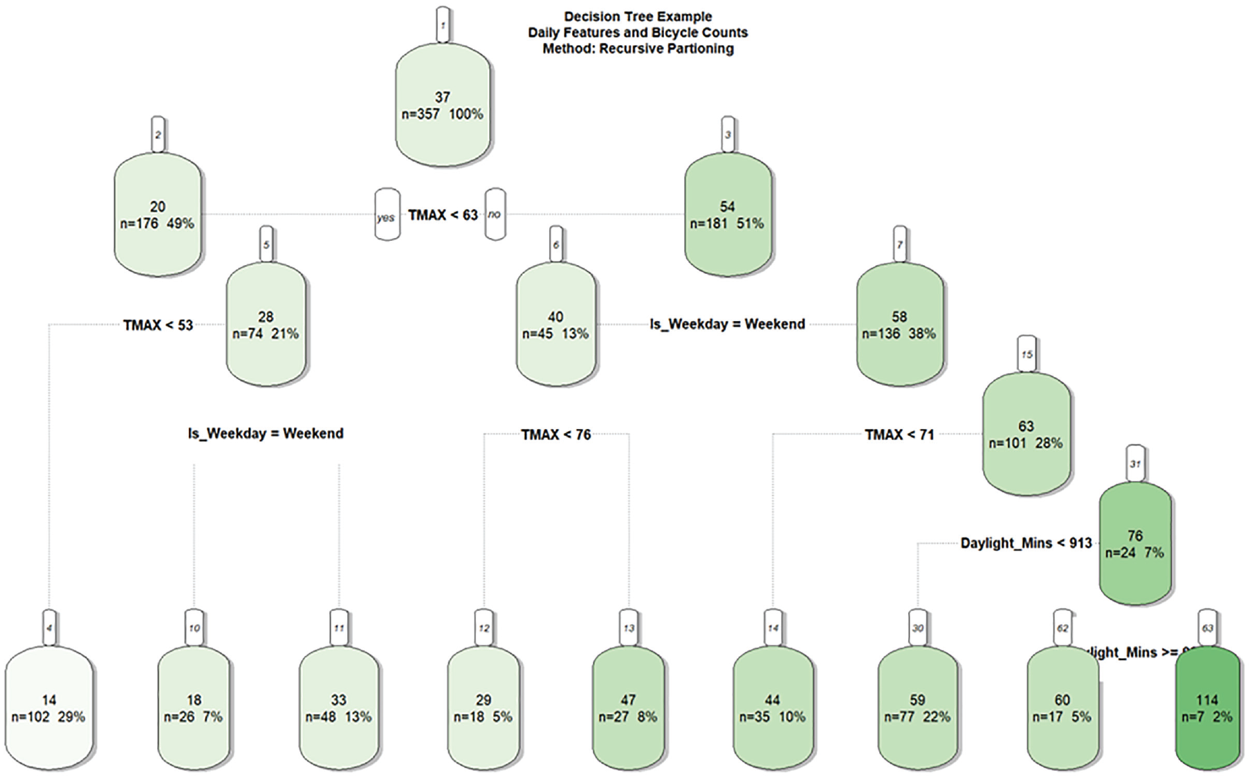
Recursive partition-based machine learning model example for daily bicycle counts imputation.

From this description it is clear that TMAX and Is_Weekday (dummy for weekend or weekday) were important variables used for splitting data at nodes. These outcomes inform the variable importance measures, where the more instances of features being used as splitting criteria the higher their variable importance measure becomes.

Now that an explanation of the variable importance measures has been given, these measures will be presented for the working models from the data imputation experiment. Because there were models estimated for multiple locations, Figure 2 summarizes these using relative representations based on color. The variable importance summary is broken down by (a) bicycle and (b) pedestrian traffic counts. This figure shows how maximum daily temperature is important for both bicycle and pedestrian traffic for all sites, albeit less so for the pedestrian Newport Avenue location. Daily precipitation and minutes of daylight were also found to be important variables for most location-specific models.

Figure 2.

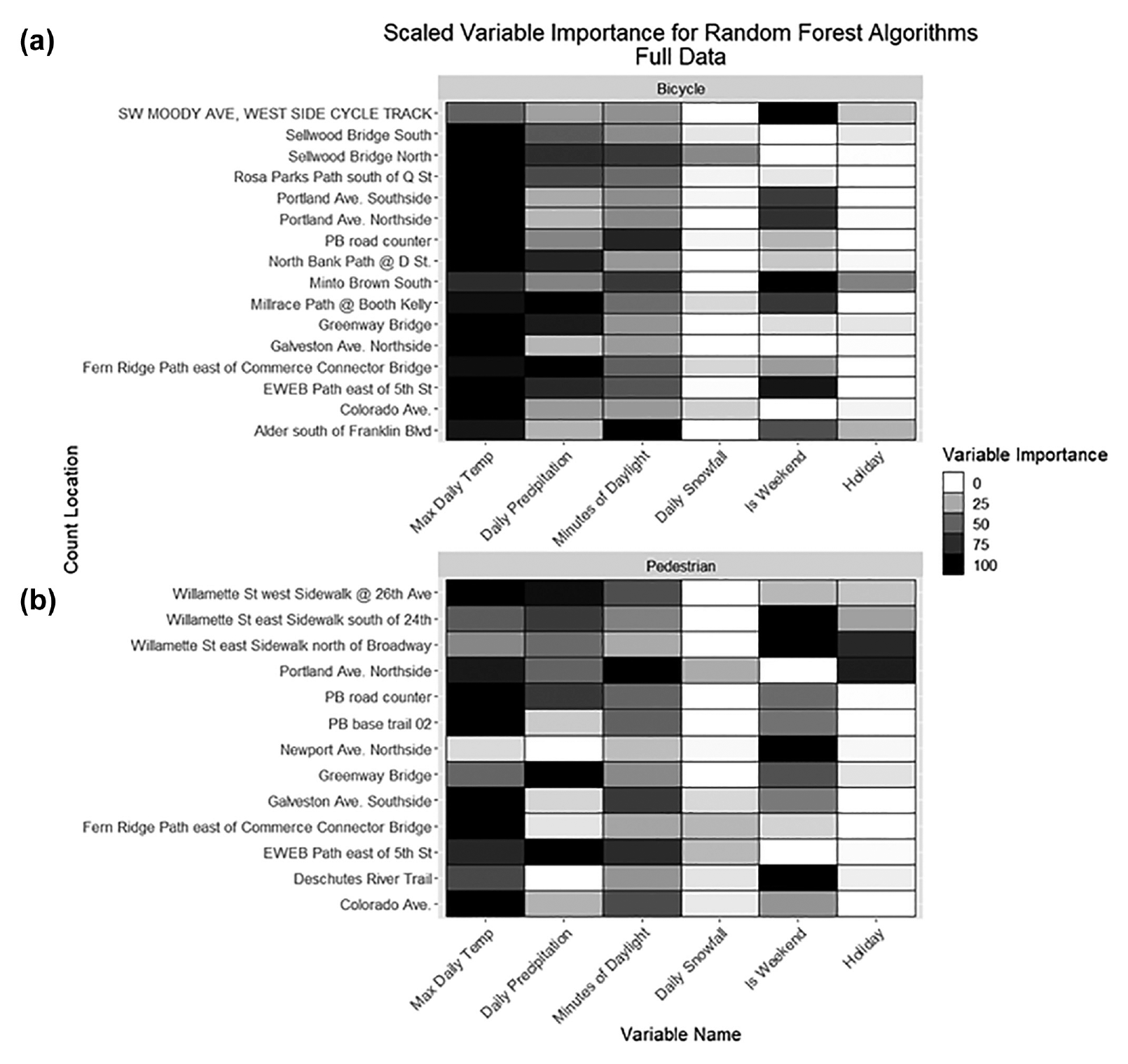
Variable importance for random forest machine learning models: (a) bicycle traffic counts and (b) pedestrian traffic counts.

Using variable importance we can check whether our models are working as expected by assessing whether the decision tree splitting variables align with the documented research and theoretical foundation. Based on the results in Figure 2 and on what has previously been documented ( 24 – 29 ) specifying the role of daily conditions and their impact on daily nonmotorized traffic counts, the models seemed to be working as expected. Presenting machine learning diagnostics, such as those in Figures 1 and 2, can also help build understanding with model users about how the model uses input features, ideally building trust with practitioners and cracking the black box pejorative of machine learning techniques.

Imputation Experimental Design

To test the efficacy of data imputation using the aforementioned methods, the experimental approach reflecteds practical imputation needs using an NMR hold design. For the statistical model and machine learning methods, daily conditions such as daily temperature, precipitation, and day of the week were used to predict the daily traffic count. What seemed to be most common in the nonmotorized count data for Oregon, were extended periods of time when the traffic sensor was either not working or not transmitting data (and forever being lost). These continuous periods of missing data informed the experimental design of the imputation tests but to simplify reporting on results, whole months were removed. The experimental design considered all possible unique combinations without replacement of months missing, which resulted in 4,094 tests for each device. Each of the 4,094 scenarios resulted in an application of each of the given imputation methods. Using a full year of counts from traffic sensors across Oregon, we simulated these missing data outages to better understand the likely error under different data outage circumstances. For instance, in Test 1 we simulated a scenario when traffic counts were available for January but missing for February through December. January data were used to train a model using the daily conditions as predictors of daily traffic counts and then the model was applied to estimate February through December (11 months) traffic counts. For the DOY factoring approach the experimental design was similar but instead of the training data being used to train a statistical or machine learning model, the test data were used like a short-duration count site where the factors from a site with correlated DOY factors within the 0.75 correlation coefficient threshold were employed to compute estimated daily and annual traffic volumes. We then compared those estimated counts from each of the methods to the actual counts and computed the absolute percent error (APE). APE is calculated using Equation 2,

APE = | \frac{AAD T_{obs} - AAD T_{est}}{AAD T_{obs}} |

(2)

where $AAD T_{obs} =$ observed daily traffic count, and $AAD T_{est} =$ estimated daily traffic count.

Imputation Experiment Data Description

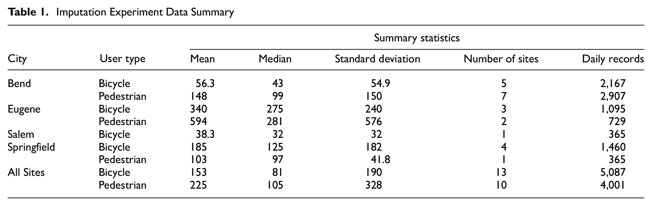
Table 1 summarizes the daily traffic count data used in this imputation experiment. Nearly 9,100 daily traffic records from years 2018 and 2019 were utilized for this research. These data were derived from 23 unique count locations throughout Oregon. Because complete annual data sets were hard to achieve, only 18 of 25 locations (combination of location and year) had a full year of data, the other eight locations had at least 351 days, or 98% of annual data. All of the count locations in this research were featured on multiuse paths. The mean values in Table 1 show that the nonmotorized traffic volumes were generally at the lower end, with Bend exhibiting the lowest counts and Eugene the highest of the data used in this research.

Table 1.

Imputation Experiment Data Summary

City	User type	Summary statistics
City	User type	Mean	Median	Standard deviation	Number of sites	Daily records
Bend	Bicycle	56.3	43	54.9	5	2,167
Bend	Pedestrian	148	99	150	7	2,907
Eugene	Bicycle	340	275	240	3	1,095
Eugene	Pedestrian	594	281	576	2	729
Salem	Bicycle	38.3	32	32	1	365
Springfield	Bicycle	185	125	182	4	1,460
Springfield	Pedestrian	103	97	41.8	1	365
All Sites	Bicycle	153	81	190	13	5,087
All Sites	Pedestrian	225	105	328	10	4,001

This research utilized supervised machine learning algorithms and regression models, relying on the documented relationships between weather, day of the week, and minutes of sunlight to predict the traffic counts ( 38 – 42 ). Historical climate data originating from the National Oceanic and Atmospheric Administration and accessed using the rnoaa library ( 43 ) were used as features in the machine learning and negative binomial regression approaches. Climate data stations for each city, typically the nearest airport, were queried and assigned to the traffic count locations nearest the station.

Imputation Experiment Results

Table 2 shows the mean APE (MAPE) and median APE for annual traffic estimation using each of the tested methods. These results were split into two groups according to whether the sites could be matched to a factor group based on the criterion recommended in Beitel et al. ( 22 ) and El Esawey ( 23 ). This process required that the daily counts were correlated with the reference group at the 0.75 level and that at least three sites were included in the reference group. If the results were based on sites that met the recommended threshold they were labeled “DOY Qualified Sites,” and those that did not meet the recommended number of sites are classified as “All Sites.” Since previous research testing the DOY factors, including the series of work by El Esawey ( 23 ) and work by Beitel et al. ( 22 ) did not include pedestrian traffic, the same criteria were not applied to the pedestrian imputation results. To ensure clarity on these points the following summary is offered:

Bicycle DOY Qualified Sites – Count sites that both met the 0.75 correlation coefficient threshold and used DOY factors from a reference group with at least three sites;

Bicycle All Sites – All sites available to this research effort including the DOY Qualified Sites with some sites only having one site included in the reference group; and

Pedestrian All Sites – All sites available to this research. Results include those that matched with reference sites at a minimum 0.40 correlation coefficient with some sites only having one site included in the reference group.

The annual results summary compared the entire year of estimates plus observed months, not just the estimate, with an observed annual count since the experiment only ever imputes 1 to 11 months of data. For instance, if the given experimental test focused on imputing January through June, by training a model on July through December, the estimated quantities used in the APE calculation would combine the January through June testing data (estimated) with the June through December training data (observed) since this is what would be done in practice. This way we can show the overall annual error when we add imputed quantities for missing data plus the remaining observed data.

The results for the bicycle traffic featured in Table 2 show that for sites that qualified for the DOY factoring method, MAPE was lowest using the negative binomial statistical model followed by the random forest and conditional inference machine learning approaches. The DOY factor approach was third best for the DOY Qualified Sites and, interestingly, when summarizing results for All Sites the DOY method marginally outperformed the other methods based on MAPE, though based on median APE, random forest performed best for the All Sites summary followed by conditional inference and recursive partitioning. For bicycle traffic estimation results, the MAPE from the negative binomial approach looked poor owing to a small number of poorly performing imputation scenarios, but the median APE showed this method was competitive with the other methods.

Table 2.

Annual Estimation Results for All Imputation Methods, Years and User Types

User type	Imputation method	DOY qualified sites		Sites analyzed	All sites		Sites analyzed
User type	Imputation method	Mean APE (%)	Median APE (%)	Sites analyzed	Mean APE (%)	Median APE (%)	Sites analyzed
Bicycle	Conditional inference	2.9	3.7	6	4.8	5.2	9
	DOY	3.3	4.0		4.2	5.4
	Negative binomial	2.4	3.1		952.0	6.5
	Random forest	2.8	3.6		4.3	4.8
	Recursive partition	5.1	4.5		4.6	5.2
Pedestrian	Conditional inference	NA			5.7	8.7	6
	DOY				9.4	13.7
	Negative binomial				96.0	8.9
	Random forest				5.5	8.1
	Recursive partition				5.8	8.6

Note: APE = absolute percent error.

Table 2 also presents results for the pedestrian traffic estimation tests. As mentioned, past research has mostly focused on missing bicycle traffic problems with less focus on missing pedestrian data problems. The best performing method based on MAPE was the random forest machine learning approach, followed closely by the conditional inference and recursive partitioning machine learning approaches with 5.5%, 5.7%, and 5.8% respectively. DOY was the next best performing method at 9.4% with the negative binomial statistical model having much higher MAPE mostly owing to some very poor performing scenarios. The overall performance ranking did not change when looking at the median error.

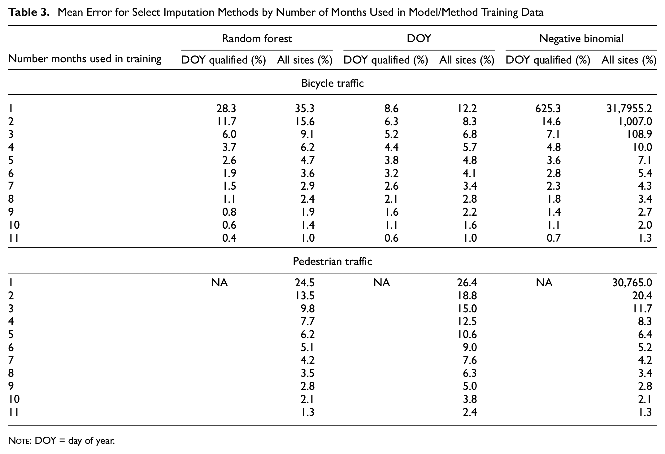
Table 3 summarizes the MAPE for selected imputation methods including the random forest machine learning method, DOY, and the negative binomial statistical model. These results were summarized based on the number of months of data used in the training. Error was summarized for sites that qualified based on previous DOY methods and for All Sites. Looking at the DOY Qualified results for bicycle traffic, the table shows that when three or fewer months of data were used in the model training the DOY approach outperformed the random forest method (and other machine learning methods, though not shown in table) and the negative binomial statistical approach. However, when four or more months of data were available the random forest approach began to outperform the DOY approach and at 5 months of training data the negative binomial approach began to outperform the DOY approach. The error from the random forest approach in the scenarios where 5 months of data or more were used was not vastly different from that of the DOY approach, though it was nearly a whole percentage point more accurate, which may not seem like a lot but if year to year variation in bicycle traffic volumes are in single digits, this level of precision is important.

Table 3.

Mean Error for Select Imputation Methods by Number of Months Used in Model/Method Training Data

Number months used in training	Random forest		DOY		Negative binomial
Number months used in training	DOY qualified (%)	All sites (%)	DOY qualified (%)	All sites (%)	DOY qualified (%)	All sites (%)
Bicycle traffic
1	28.3	35.3	8.6	12.2	625.3	31,7955.2
2	11.7	15.6	6.3	8.3	14.6	1,007.0
3	6.0	9.1	5.2	6.8	7.1	108.9
4	3.7	6.2	4.4	5.7	4.8	10.0
5	2.6	4.7	3.8	4.8	3.6	7.1
6	1.9	3.6	3.2	4.1	2.8	5.4
7	1.5	2.9	2.6	3.4	2.3	4.3
8	1.1	2.4	2.1	2.8	1.8	3.4
9	0.8	1.9	1.6	2.2	1.4	2.7
10	0.6	1.4	1.1	1.6	1.1	2.0
11	0.4	1.0	0.6	1.0	0.7	1.3
Pedestrian traffic
1	NA	24.5	NA	26.4	NA	30,765.0
2		13.5		18.8		20.4
3		9.8		15.0		11.7
4		7.7		12.5		8.3
5		6.2		10.6		6.4
6		5.1		9.0		5.2
7		4.2		7.6		4.2
8		3.5		6.3		3.4
9		2.8		5.0		2.8
10		2.1		3.8		2.1
11		1.3		2.4		1.3

Note: DOY = day of year.

Evaluating the All Sites results showed a similar story, with the DOY method outperforming the other methods when four or fewer months of data were available for training. The negative binomial method performed especially weakly when only 1 month of data were available, probably a result of the inability of the statistical model to make decent inferences for warm, high volume months when using data from months of the year that exhibit low volumes owing to the cold and rain. An in-depth review of the extremely high error results showed single month training scenarios most often used the months of January, February, or December and the estimated model parameters had counterintuitive signs and strength.

The results presented in Table 3also show the results for the pedestrian traffic imputation experiments. These results showed that the random forest approach outperformed the DOY and negative binomial statistical approaches no matter how many months were used in the training of the model. The difference between the random forest and DOY methods for pedestrian traffic was more distinct than for the bicycle traffic, likely owing to the lower threshold used to match the sites to reference groups in the DOY factoring process.

A helpful way to look at the imputation results for practitioners is to look at the likely upper bound of the estimation error to determine the worst case error. The results in Figure 3 present the 95th percentile error results of all imputation tests based on the number of months used in the training of each imputation approach. This chart essentially shows how 95% of the imputation experiments performed for each method. The results in the figure are for the random forest and DOY methods; the DOY Qualified and All Sites scenarios are also presented. For bicycle traffic, the DOY method outperformed the random forest approach when just 1 or 2 months were used in the training; when 3 months of data were available, the random forest began to outperform the DOY method. Looking at the DOY Qualified Sites the DOY method stagnated at about 20% error from 2 through 4 months of data used in the method, whereas the random forest method improved from 41% error to 9% error. The 95th percentile error results for pedestrian traffic showed that the random forest method outperformed the DOY method for all scenarios presented.

Figure 3.

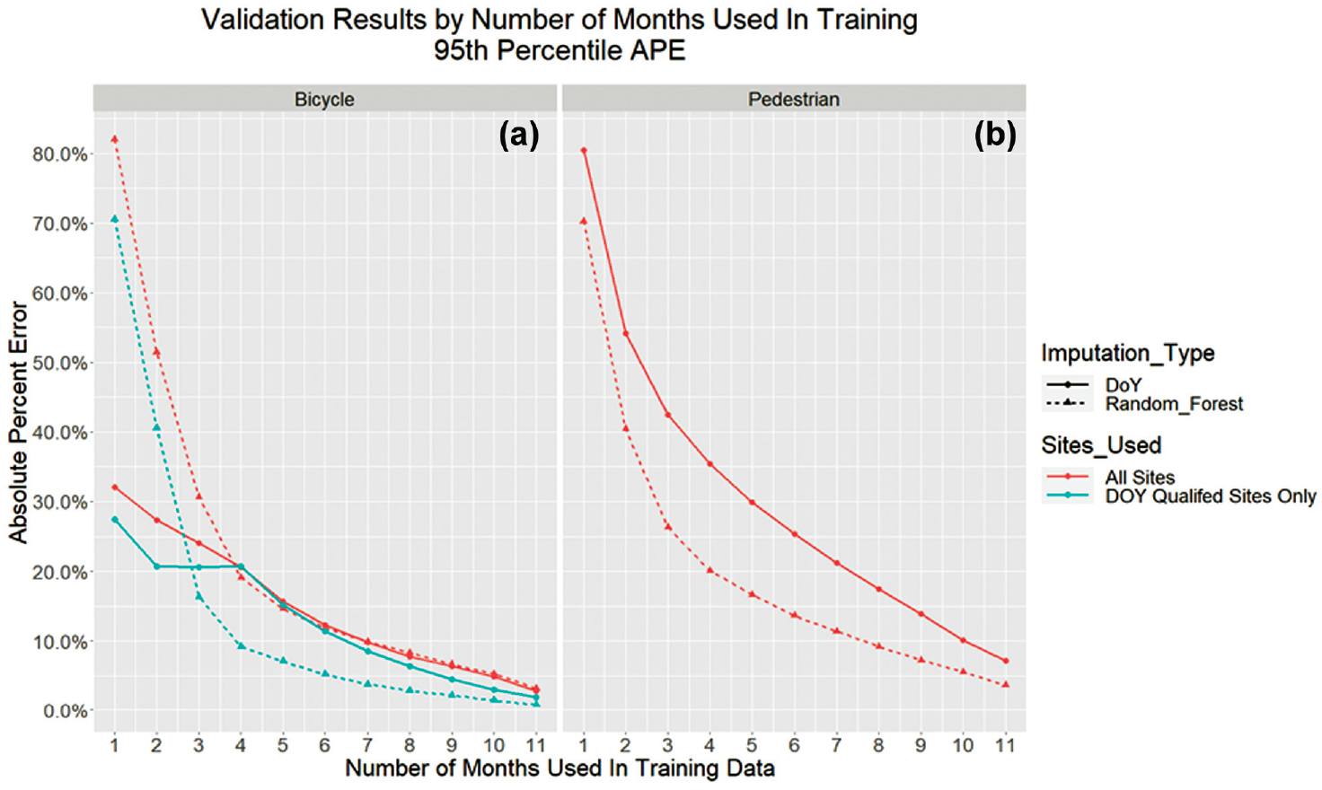
Imputation results for DOY and random forest at 95th percentile – comparing number of months in training data: (a) bicycle and (b) pedestrian.

Discussion and Recommendations for Count Program Application

There is a significant need for reliable methods to impute nonmotorized traffic data since traffic sensors experience frequent technical issues resulting in data loss and for many nonmotorized traffic programs with fewer dedicated staff to monitor hardware health data, data outages are likely to be higher. Multiple imputation methods were tested in this study including simplistic DOY factoring and more sophisticated statistical and machine learning models.

Table 4 summarizes the strengths and weaknesses of the DOY and random forest machine learning approaches. The DOY factors worked well, their simplicity notwithstanding, but the ability to apply these methods to all available sites was hampered by the current criteria guiding their application, specifically that they require the ability to match with a reference site group using correlation analysis, and that those groups should have at least three sites. It was found that when these criteria were not met accuracy was affected, as expected, and thus made the DOY less flexible to apply in practice. An example of this inflexibility was that none of the pedestrian traffic sites met the recommended criteria for applying the DOY and so, in practice, without an alternative solution, those sites would be left with data gaps. Another criterion that Beitel et al. recommended was that only sites with an AADT of 250 or more be considered when applying the DOY method, which would mean that none of the sites used would have qualified ( 22 ). However, this research demonstrated that the 250 AADT threshold is probably not necessary considering the accuracy from the DOY approach presented in this research.

Table 4.

Strengths and Weaknesses of DOY and Random Forest Imputation Method

DOY method	Random forest method
Strengths
Accurate for most missing data situations	Accurate in low through moderate missing data scenarios
Simple method to understand and apply	More flexible, does not require partner sites to apply
	Improves with multiple years of data available
	Less sensitive to particular months missing form training data
Weaknesses
Less flexible, requires multiple partner sites with similar temporal patterns	More complicated to estimate and apply
Less accurate in certain missing data scenarios	Less accurate in very high missing data scenarios
Does not benefit from multiple years of data available	Sensitive to combination of months used
More sensitive to certain months not used in factor development	Sensitive to combination of months used

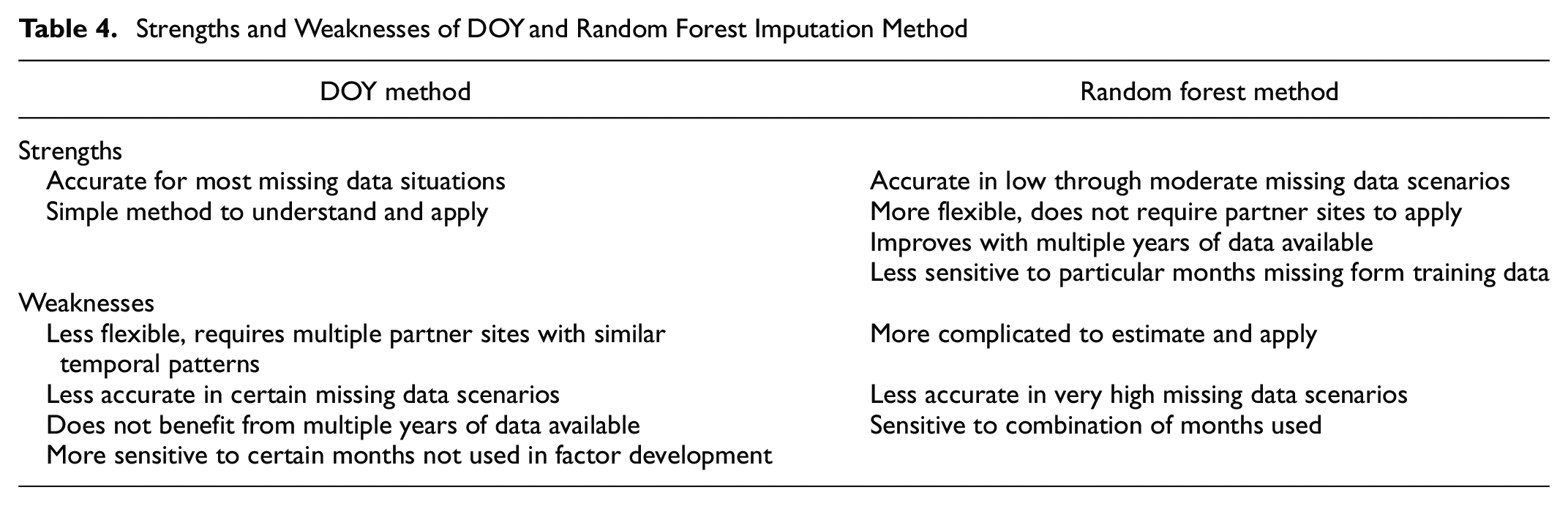
A major strength of the DOY method is its simplicity, which makes application more likely in public agencies in which data scientist job classifications are rare. However, the random forest imputation approach offers a number of advantages including higher accuracy in low to moderate missing data scenarios. Though this accuracy is just a percentage point or so, this could mean the difference in accurately accounting for small changes in travel demand that might be experienced at many sites for nonmotorized travel. And though the random forest model performed less well in low data scenarios, in practice such a scenario may not ever take place since machine learning approaches (as well as parametric approaches) can utilize information from multiple years of data. This research only tested scenarios for which 1 year of data was used in both training and testing data sets, but in practice it is likely that a previous year’s data or many previous years’ worth of data would be available to add to the training data and make high missing data situations uncommon. This highlights one of the DOY weaknesses in that the method does not improve with multiple years of data, whereas the random forest model would conceivably grow in power as more years of data are fed into the training process. Future research should explore this potential strength in more detail. The last item to consider the sensitivity of the DOY method to the particular months used in factor development and the random forest appraoch needing data from months that represent well, the weather conditions throughout the time period being estimated. Whereas the DOY method can be impacted by a high volume month like May or October, random forest model is less sensitive to these missing data scenarios but would struggle if missing all the months with little precipitation and thus more sensitive to the combination of months used. Depending on the missing data scenario this could play in favor of one method over the other.

This research compares favorably with other bicycle traffic imputation research. Though El Esawey tested different missing data scenarios, that research resulted in 10% MAPE when 30% of the data were missing, whereas this research’s most comparable scenario was when 8 to 9 months of data were missing ( 23 ). The random forest and DOY methods resulted in MAPEs of 6.0% and 5.2% respectively for missing 9 months (25% missing data) of data and 3.7% and 4.4% respectively for missing 8 months (34.4% missing data).

This research also summarized measures of variable importance to help illuminate the black box perception of machine learning in the hope of building more acceptance from practitioners. Another barrier to widespread adoption of machine learning imputation techniques is the lack of agency staff with the data science skills necessary to estimate and apply these more complicated methods. Though estimated and applied in the R open source statistical computing environment, adaption to existing traffic count database architecture would probably require traffic count database vendor acceptance. This research offers documented pathways for implementing data imputation methods in agency run nonmotorized traffic count programs.

Footnotes

Author Contributions

The author confirms sole responsibility for the following: study conception and design, data collection, analysis and interpretation of results, and manuscript preparation.

Declaration of Conflicting Interests

The author declared no potential conflicts of interest with respect to the research, authorship, and/or publication of this article.

Funding

The author received no financial support for the research, authorship, and/or publication of this article.

References

Federal Highway Administration. Traffic Monitoring Guide. FHWA-PL-95-031. U.S. Department of Transportation, Federal Highway Administration, Office of Highway Information Management, 2016. https://www.fhwa.dot.gov/policyinformation/tmguide/tmg_fhwa_pl_17_003.pdf

New Mexico State Highway and Transportation Department. 1990 Survey of Traffic Monitoring Practices among State Transportation Agencies of the United States. Report No. FHWA-HRP-NM-90-05. New Mexico State Highway and Transportation Department, Santa Fe, 1990.

ASTM E2759-10. Standard Practice for Highway Traffic Monitoring Truth-in-Data. ASTM International, West Conshohocken, PA, 2018. www.astm.org.

Al-Deek

H. M.

Venkata

Chandra

S. R.

New Algorithms for Filtering and Imputation of Real-Time and Archived Dual-Loop Detector Data in I-4 Data Warehouse. Transportation Research Record: Journal of the Transportation Research Board, 2004. 1867: 116–126.

Leonard

J. D.

Guin

Feng

Multiple Imputation Scheme for Overcoming the Missing Values and Variability Issues in ITS Data. Journal of Transportation Engineering, Vol. 131, No. 12, 2005, pp. 931–938.

Zhong

Sharma

Liu

Assessing Robustness of Imputation Models Based on Data from Different Jurisdictions: Examples of Alberta and Saskatchewan, Canada. Transportation Research Record: Journal of the Transportation Research Board, 2005. 1917: 116–126.

Turner

Park

E. S.

Incomplete Archived Data of Intelligent Transportation Systems for Calculation of Annual Average Traffic Statistics: What Level of Missing Data Causes Problems?

Transportation Research Record: Journal of the Transportation Research Board, 2008. 2049: 1–13.

Box

Jenkins

Time Series Analysis: Forecasting and Control. Holden-Day, San Francisco, 1970.

Chatfield

The Analysis of Time Series: An Introduction, 4th ed. Chapman and Hall, New York, 1989.

10.

Castro-Neto

Jeong

M. K.

Han

L. D.

AADT Prediction Using Support Vector Regression with Data-Dependent Parameters. Expert Systems with Applications, Vol. 36, No. 2, 2009, pp. 2979–2986. https://doi.org/10.1016/j.eswa.2008.01.073

11.

Zhong

Sharma

Lingras

Genetically Designed Models for Accurate Imputation of Missing Traffic Counts. Transportation Research Record: Journal of the Transportation Research Board, 2004. 1879: 71–79.

12.

Tight

M. R.

Redfern

E. J.

Watson

S. M.

Clark

S. D.

Outlier Detection and Missing Value Estimation in Time Series Traffic Count Data: Final Report of SERC Project GR/G23180. Working Paper 401. Institute of Transport Studies, University of Leeds, UK, 1993. https://eprints.whiterose.ac.uk/2174/1/ITS295_WP401_uploadable.pdf

13.

Nordback

Marshall

Janson

Stolz

Estimating Annual Average Daily Bicyclists: Error and Accuracy. Transportation Research Record: Journal of the Transportation Research Board, 2013. 2339: 90–97.

14.

Beitel

Miranda-Moreno

Methods for Improving and Automating the Estimation of Average Annual Daily Bicyclists. Presented at 95th Annual Meeting of the Transportation Research Board, Washington, D.C., 2016.

15.

Nordback

Kothuri

Johnstone

Lindsey

Ryan

Raw

Minimizing Annual Average Daily Nonmotorized Traffic Estimation Errors: How Many Counters Are Needed Per Factor Group?

Transportation Research Record: Journal of the Transportation Research Board, 2019. 2673: 295–310.

16.

El Esawey

Lim

Sayed

Mosa

A. I.

Development of Daily Adjustment Factors for Bicycle Traffic. Journal of Transportation Engineering, Vol. 139, No. 8, 2013, pp. 859–871.

17.

El Esawey

Estimation of Annual Average Daily Bicycle Traffic with Adjustment Factors. Transportation Research Record: Journal of the Transportation Research Board, 2014. 2443: 106–114.

18.

El Esawey

Impact of Data Gaps on the Accuracy of Annual and Monthly Average Daily Bicycle Volume Calculation at Permanent Count Locations. Computers, Environment, and Urban Systems, Vol. 70, 2018, pp. 125–137.

19.

El Esawey

Toward a Better Estimation of Annual Average Daily Bicycle Traffic: Comparison of Methods for Calculating Daily Adjustment Factors. Transportation Research Record: Journal of the Transportation Research Board, 2016. 2593: 28–36.

20.

Hankey

Lindsey

Marshall

Day-of-Year Scaling Factors and Design Considerations for Nonmotorized Traffic Monitoring Programs. Transportation Research Record: Journal of the Transportation Research Board, 2014. 2468: 64–73.

21.

Nosal

Miranda-Moreno

L. F.

Krstulic

Incorporating Weather: Comparative Analysis of Annual Average Daily Bicyclist Traffic Estimation Methods. Transportation Research Record: Journal of the Transportation Research Board, 2014. 2468: 100–110.

22.

Beitel

McNee

McLaughlin

Miranda-Moreno

L. F.

Automated Validation and Interpolation of Long-Duration Bicycle Counting Data. Transportation Research Record: Journal of the Transportation Research Board, 2018. 2672: 75–86.

23.

El Esawey

Daily Bicycle Traffic Volume Estimation: Comparison of Historical Average and Count Models. Journal of Urban Planning and Development, Vol. 144, No. 2, 2018, p. 04018011.

24.

El Esawey

Moda

Nasr

Estimation of Daily Bicycle Traffic Volumes Using Sparse Data. Computers, Environment and Urban Systems, Vol. 54, 2015, pp. 195–203.

25.

El Esawey

Estimation of Daily Bicycle Traffic Volumes using Spatiotemporal Relationships. Journal of Transportation Engineering, Part A: Systems, Vol. 143, No. 11, 2017, p. 04017056.

26.

Roll

J. F.

Proulx

F. R.

Estimating Annual Average Daily Bicycle Traffic without Permanent Counter Stations. Transportation Research Record: Journal of the Transportation Research Board, 2018. 2672: 145–153.

27.

Díaz-Uriarte

de Andrés

S. A.

Gene Selection and Classification of Microarray Data Using Random Forest. BMC Bioinformatics, Vol. 7, 2006, p. 3.

28.

Heidema

A. G.

Boer

J. M. A.

Nagelkerke

Mariman

E. C. M.

Feskens

E. J. M.

The Challenge for Genetic Epidemiologists: How to Analyze Large Numbers of SNPs in Relation to Complex Diseases. BMC Genetics, Vol. 7, 2006, p. 23.

29.

Ryo

Rillig

M. C.

Statistically Reinforced Machine Learning for Nonlinear Patterns and Variable Interactions. Ecosphere, Vol. 8, No. 11, 2017, p. e01976.

30.

Hothorn

Hornik

van de Wiel

M. A.

Zeileis

A Lego System for Conditional Inference. American Statistician, Vol. 60, 2006, pp. 257–263.

31.

Strobl

Boulesteix

A.-L.

Kneib

Augustin

Zeileis

Conditional Variable Importance for Random Forests. BMC Bioinformatics, Vol. 9, 2008, p. 307. https://doi.org/10.1186/1471-2105-9-307

32.

Bauer

Kohavi

An Empirical Comparison of Voting Classification Algorithms: Bagging, Boosting, and Variants. Machine Learning, Vol. 36, No. 1–2, pp. 105–139.

33.

Breiman

Bagging Predictors. Machine Learning, Vol. 24, No. 2, 1996, pp. 123–140.

34.

Dietterich

T. G.

An Experimental Comparison of Three Methods for Constructing Ensembles of Decision Trees: Bagging, Boosting, and Randomization. Machine Learning, Vol. 40, No. 2, 2000, pp. 139–157.

35.

Tang

Ishwaran

Random Forest Missing Data Algorithms. Statistical Analysis and Data Mining, Vol. 10, No. 6, 2017, pp. 363–377. https://doi.org/10.1002/sam.11348

36.

Kuhn

Wing

Weston

Williams

Keefer

Engelhardt

Cooper

Mayer

Kenkel

Lescarbeau

Ziem

Scrucca

Tang

Candan

Hunt

caret: Classification and Regression Training. R Package Version 6.0-84. https://CRAN.R-project.org/package=caret.

37.

Venables

W. N.

Ripley

B. D.

Modern Applied Statistics with S, 4th ed. Springer, New York, 2002.

38.

Miranda-Moreno

L. F.

Nosal

Weather or Not to Cycle: Temporal Trends and Impact of Weather on Cycling in an Urban Environment. Transportation Research Record: Journal of the Transportation Research Board, 2011. 2247: 42–52.

39.

Tin

S. T.

Woodward

Robinson

Ameratunga

Temporal, Seasonal and Weather Effects on Cycle Volume: An Ecological Study. Environmental Health: A Global Access Science Source, Vol. 11, 2012, p. 12.

40.

Rose

Ahmed

Figliozzi

Jakob

Quantifying and Comparing Effects of Weather on Bicycle Demand in Melbourne, Australia, and Portland, Oregon. Presented at 90th Transportation Research Board Annual Meeting, Transportation Research Board of the National Academics, Washington, D.C., 2011.

41.

Lewin

Temporal and Weather Impacts on Bicycle Volumes. Transportation Research Record: Journal of the Transportation Research Board, 2011. 2536: 42–52.

42.

Nosal

Miranda-Moreno

L. F.

Cycling and Weather: A Multi-City and Multi-Facility Study in North America. Presented at 91st Annual Meeting of the Transportation Research Board, Transportation Research Board of the National Academics, Washington, D.C., 2012.

43.

Chamberlain

rnoaa: ‘NOAA’ Weather Data from R. R Package Version 0.9.4, 2019. https://CRAN.R-project.org/package=rnoaa.

44.

Guyon

Elisseeff

An Introduction to Variable and Feature Selection. Journal of Machine Learning Research, Vol. 3, 2003, pp. 1157–1182. https://doi.org/10.1162/153244303322753616