Novel Algorithm for Mutual Alignment of Railway Track Geometry Measurements

Abstract

Track geometry measurements are regularly collected to monitor the condition of a railway network. To detect deterioration patterns and enable predictive maintenance, sequential measurement runs must be mutually aligned which has been proven a serious challenge. This paper presents a novel algorithm for mutual alignment of track geometry signal data. It resolves several previously intractable alignment problems: highly segmented data with variable sample rate, spatially correlated and uncorrelated measurement errors, convergence to true locations, and consistency over time. The algorithm adjusts spatial measurement errors by splitting signals in continuous segments. Re-sampled, error-corrected signals are mutually aligned using cross correlation, and this process is repeated until the mutual alignment meets a pre-defined precision threshold. Missing measurement values are handled by imputing an interpolated offset from nearby segments, ensuring that the signals remain continuous. By using weighted average offsets over all aligned signals, the law of large numbers guarantees convergence and consistency. The practical feasibility of the algorithm is demonstrated on empirical track geometry measurement data from the British railway network, owned and operated by Network Rail.

In order for railway networks to meet higher standards of service level and safety, condition monitoring and predictive maintenance are becoming increasingly important. Collection of track geometry data is an established procedure to facilitate evaluation of the functional condition and deterioration patterns of the railway track ( 1 – 3 ). Track geometry data are normally collected from sensors, either on dedicated track recording vehicles or on in-service vehicles. Sensor measurement indicators, techniques, and accuracy are well-studied and constantly improving topics. Some recent examples on advancements in the railway sector include replacement condition detection of railway points ( 4 ), degradation of railway crossings ( 5 ), image-based detection of track geometric parameters ( 6 ), fault diagnostics of railway axle bearings ( 7 ), image detection of fasteners ( 8 ), machine learning for analyzing the effect of geocell installation on track geometry quality ( 9 ), and novel filtering and smoothing algorithms for railway track surveying ( 10 ). However, predictive models usually need data from sequential condition monitoring runs to estimate deterioration patterns. As stated by Weston et al: ( 11 ) “Mutually aligning data is critical for obtaining the changes in track condition over time. Mutual alignment of data from different runs over the same track presents a serious challenge.” These challenges are present in monitoring systems based on both tachometers and global navigation satellite systems (GNSS). For tachometers, Weston et al. ( 11 ) points out that a slightly different wheel radius will cause an accumulation of distance errors. For GNSS-positioning, various sources of measurement errors occur, including, for example, clock-related errors, signal propagation errors, receiver noise, signal jamming, and signal spoofing ( 12 ).

Previous studies have dealt with alignment of multiple signals in different ways. Common techniques to improve accuracy in positioning of condition measurements are data fusion between GNSS and INS (inertial navigation systems), on which there is extensive research ( 13 , 14 ). Another technique to identify the actual position of a train or measurement is map matching ( 15 , 16 ). Both of these methods can improve the position accuracy of a single run, and thus significantly simplify the process of mutually aligning several measurement runs. However, according to Al-Douri and Tretten ( 17 ), existing studies have not adequately dealt with the problem of sufficient mutual alignment from a maintenance decision-making point of view.

To further improve alignment, post-processing algorithms can be imposed. In his dissertation, Faiz evaluates three different algorithms for mutually aligning track geometry data: distance alignment, fixed-window-based alignment, and parameter-based alignment. Faiz et al. ( 18 ) conclude that the latter provides the most accurate signal data alignment. The parameter-based alignment finds the closest match for each parameter value by incrementally shifting each parameter one row and calculating the minimum absolute error over time. This method works well when the signals have an overlap between different runs, but signal measurements from disjoint segments of a railway track will not be well aligned. As non-overlapping segments are very common in practice, an algorithm intended to work in a predictive maintenance setting needs to address this issue.

Bergquist et al. ( 19 ) conclude that pattern matching between runs, and then the use of the average location for all measurements, is a straightforward alignment algorithm in theory. However, because of post-processing, measurement errors, differences in measurement equipment, and potential loss of data in the collection process, alignment in this fashion faces significant problems. They also propose that for regular maintenance, the exact location of point defects is not as important as monitoring deterioration of an extended segment ( 19 ).

Even though the exact location of a defect is not a requirement for predictive maintenance, the mutual alignment algorithm must ensure a location estimate that is accurate enough to enable maintenance actions on the track. Al-Douri and Tretten ( 17 ) state that current research has not yet solved this issue: “Overall, data are inaccurate, there is no testing phase using realistic data, and existing models are insufficient. This has a negative impact on maintenance decisions.”

We address these concerns by proposing an algorithm for mutual alignment of sensor measurement data of track geometry parameters. Novel aspects of the algorithm are:

Alignment of highly segmented data, that is, aligning signals which do not necessarily have an overlap with other signals.

Alignment of data with variable sample rate.

Alignment of data with various aspects of measurement errors, spatial errors, missing locations, and missing measurements.

Alignment ensuring convergence toward the true location.

Alignment which is consistent over time, that is, data are aligned even after maintenance has occurred and changed the track geometry.

In summary, the algorithm presents a working method to align large amounts of track geometry data, in spite of measurement errors and/or missing data which are common in practice. The algorithm addresses several issues pointed out in available literature, such as accuracy and practical feasibility. To our knowledge, no previous method has resolved all of the above stated issues.

Materials and Methods

Data Material

The algorithm described in this paper is used to align real track geometry data from the British railway network, owned and operated by Network Rail. The example data was collected from Network Rail’s Engineer’s Line References (ELR) VTB3 1100, going from Earlswood mileage change to Brighton. Measurements were made between June 26, 2017 and July 1, 2019. In total, this dataset consists of 20 measurement runs, ranging from 2,047 m to 46,775 m in length.

The track geometry data is collected by Network Rail’s fleet of track recording vehicles. Measurements are pre-processed using data fusion between an onboard RTPS (real time positioning system) and map matching. The RTPS consists of D-GPS (differential global positioning system), inertial measurement unit, and tachometer. Spatial positions of each query run are derived and map matched to an integrated network map, the route setting (RS) files, providing information about the route. The reference RS files may not align fully to RTPS which can cause inaccurate distances.

Because measurement vehicle layout is different, the reference position of each track geometry system and RTPS varies between vehicles. In practice, trains running in the same orientation show a more consistent alignment when data is overlaid. However, recordings of the same section of track result in locations varying several meters between runs from the same vehicle running in a different orientation, or different vehicles in running in different orientations.

Track geometry measurements are spatially sampled approximately every 200 mm by a tachometer which is independent of the GPS providing its location. Each data point receives an applied position that may or may not equate to 200 mm. Recording vehicles will also have different tachometer counts, causing initial unpredictable drifts, which the RTPS tries to compensate for. The GPS-positioning adjusts the location continuously, which means it sometimes re-adjusts locations, causing visual overlaps in the signal measurements.

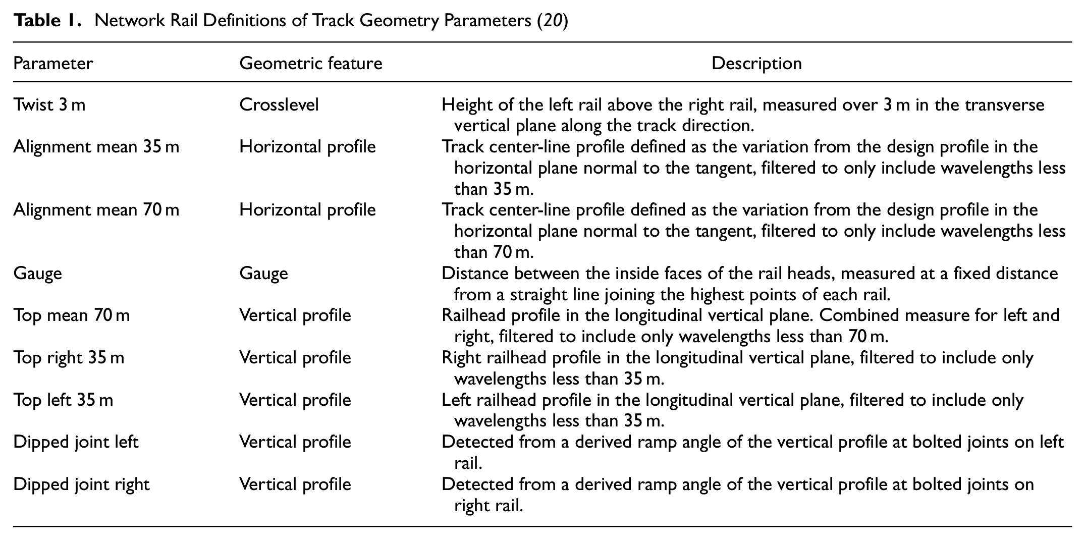
Table 1 describes nine track geometry parameters which are aligned using the proposed algorithm.

Table 1.

Network Rail Definitions of Track Geometry Parameters ( 20 )

Parameter	Geometric feature	Description
Twist 3 m	Crosslevel	Height of the left rail above the right rail, measured over 3 m in the transverse vertical plane along the track direction.
Alignment mean 35 m	Horizontal profile	Track center-line profile defined as the variation from the design profile in the horizontal plane normal to the tangent, filtered to only include wavelengths less than 35 m.
Alignment mean 70 m	Horizontal profile	Track center-line profile defined as the variation from the design profile in the horizontal plane normal to the tangent, filtered to only include wavelengths less than 70 m.
Gauge	Gauge	Distance between the inside faces of the rail heads, measured at a fixed distance from a straight line joining the highest points of each rail.
Top mean 70 m	Vertical profile	Railhead profile in the longitudinal vertical plane. Combined measure for left and right, filtered to include only wavelengths less than 70 m.
Top right 35 m	Vertical profile	Right railhead profile in the longitudinal vertical plane, filtered to include only wavelengths less than 35 m.
Top left 35 m	Vertical profile	Left railhead profile in the longitudinal vertical plane, filtered to include only wavelengths less than 35 m.
Dipped joint left	Vertical profile	Detected from a derived ramp angle of the vertical profile at bolted joints on left rail.
Dipped joint right	Vertical profile	Detected from a derived ramp angle of the vertical profile at bolted joints on right rail.

Algorithm

Figure 1 provides a flow chart of the algorithm. Examples of alignment performance are presented in in a case study in the Results section.

Figure 1.

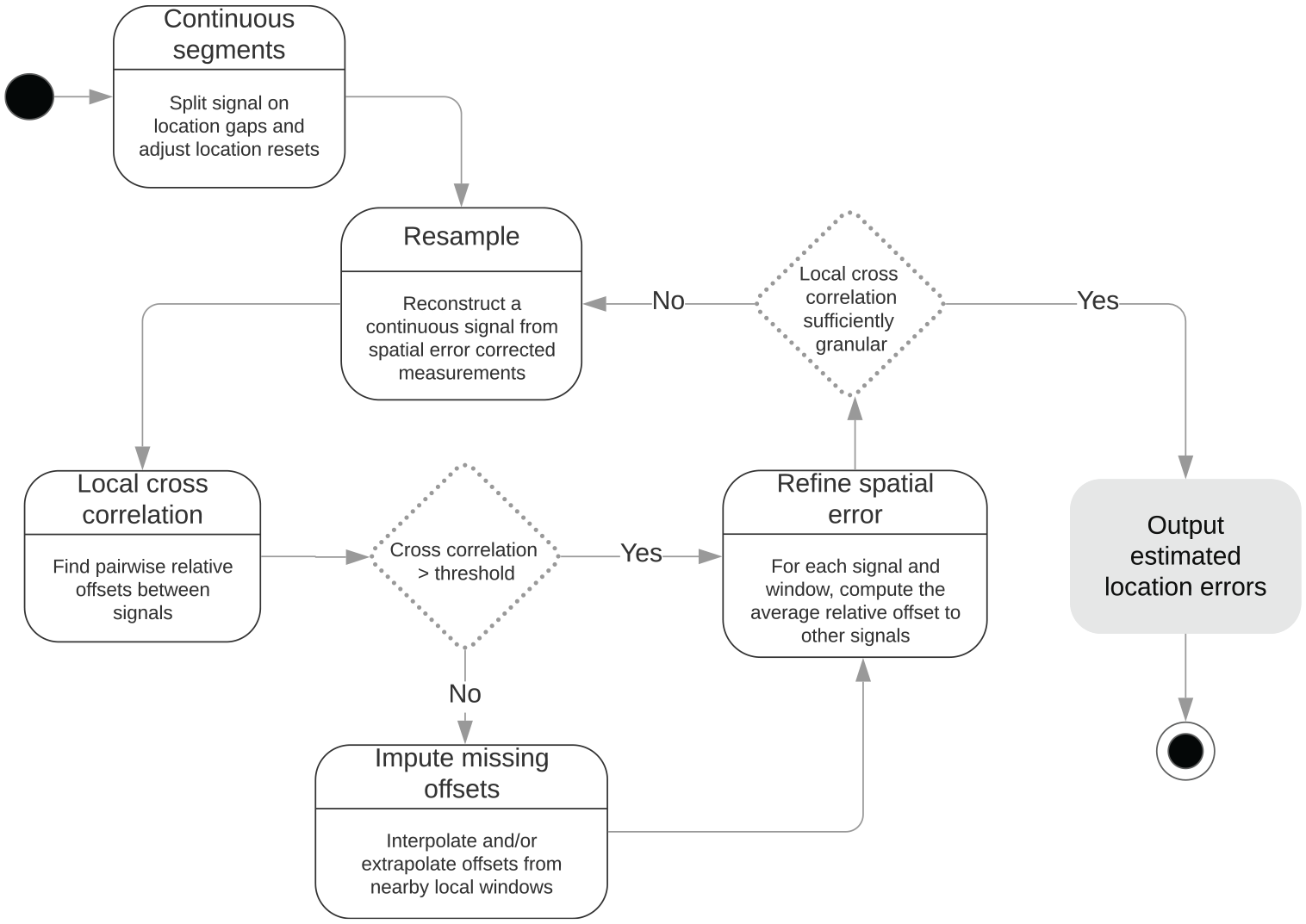
Flow chart for the alignment algorithm.

Sampling

The true signal sampled by the track measurement equipment is modeled as a continuous function of location $\hat{y} (\hat{x})$ and band-limited with an upper bound of $f_{s} / 2$ . This signal is piecewise sampled at an approximate sample rate $f_{s}$ in a series of observations $(x [i], y [i]), i \in N$ with errors in both value measurement $γ [i]$ and spatial measurement $ϵ [i]$ :

\hat{y} (x [i] - ϵ [i]) = y [i] - γ [i] = \hat{y} [i]

(1)

Repeated measurements form a time series of signals ${\hat{y}}_{1} (\hat{x}), {\hat{y}}_{2} (\hat{x}), \dots$ where overlapping segments can describe degradation in railway track quality over time. Our method estimates the spatial measurement error $\hat{ϵ}$ to mutually align signals. We assume that errors in value measurement $γ = y - \hat{y}$ are iid (independent identically distributed) and make no attempts at estimating them here.

The signal of every track geometry parameter is sampled unevenly, and with occasional spatial gaps between measurements. The spatial measurement errors $ϵ$ have a tendency to drift and are thus spatially correlated. The spatial errors can also make sudden smaller jumps without breaking the continuity of the modeled signal $\hat{y}$ .

Continuous Segments

To simplify processing and notation we split a sampled signal into segments and model continuous pieces of the full continuous signal. In each a segment a zeroth order location estimate ${\hat{x}}_{0}$ has a step size that approximately corresponds to the sample rate $f_{s}$ .

Δ {\hat{x}}_{0} [i] \approx 1 / f_{s}

(2)

{\hat{x}}_{0} [i] = x [i] - \hat{ϵ} [i]

(3)

where $Δ x [i]$ is defined as the forward finite difference:

Δ x [i] : = x [i + 1] - x [i]

(4)

Gaps

A sample may have gaps that are not explicitly marked in the sequence of observations. Such gaps can, however, be identified by verifying that the distance to the next location is much greater than expected with Inequality 5 or, more specifically, Inequality 6:

Δ x [i] >> 1 / f_{s}

(5)

Δ x [i] > T_{g}

(6)

where $T_{g}$ is a threshold configuration parameter defining where a sample signal is split into segments representing a continuous piece of the signal. In subsequent sections we assume that a sample x has no gaps.

Location Resets

As the tachometer sequentially samples a signal y, the RTPS records the location x. The RTPS has a correction mechanism that periodically resets the location, which causes sudden jumps in the location sequence even though the track recording vehicle is steadily moving in one direction (see detailed description in the Materials and Methods section). Such jumps are characterized by an unexpected distance between two consecutive observations (Inequality 7). These sudden jumps can even make the measurement locations non-monotonic ( $Δ x [i] < 0$ ) as illustrated in Figure 2.

Δ x [i] ≉ 1 / f_{s}

(7)

When the situation represented by Inequality 7 is detected a fixed step size is imputed in the estimated location:

Δ \hat{x} [i] \approx 1 / f_{s}

Δ \hat{x} [i] = {\begin{matrix} Δ x [i], if Δ x [i] \approx 1 / f_{s} \\ 1 / f_{s} \end{matrix}

This implies that the estimated error $\hat{ϵ} [i]$ at each observation i affects the next error estimate $\hat{ϵ} [i + 1]$ :

\begin{matrix} Δ x [i] ≉ 1 / f_{s} \Rightarrow \\ Δ \hat{x} [i] = 1 / f_{s} \Leftrightarrow \\ Δ x [i] - Δ \hat{ϵ} [i] = 1 / f_{s} \Leftrightarrow \\ Δ \hat{ϵ} [i] = Δ x [i] - 1 / f_{s} \Leftrightarrow \\ \hat{ϵ} [i + 1] - \hat{ϵ} [i] = Δ x [i] - 1 / f_{s} \Leftrightarrow \\ \hat{ϵ} [i + 1] = \hat{ϵ} [i] + Δ x [i] - 1 / f_{s} \end{matrix}

(8)

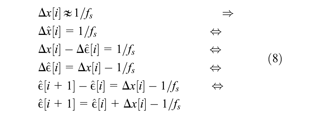
We construct an estimated location $\hat{x}$ by recursively adding up potentially adjusted errors in both the forward direction ${\hat{ϵ}}_{f}$ and the backward direction ${\hat{ϵ}}_{b}$ . We make no assumption about whether the position is more accurate before or after a position reset, or even if the value before or after is the new location reset by the RTPS.

\begin{matrix} {\hat{ϵ}}_{f} [i + 1] = {\hat{ϵ}}_{f} [i] + {\begin{matrix} 0 Δ x [i] \approx 1 / f_{s} \\ Δ x [i] - 1 / f_{s} \end{matrix} \\ {\hat{ϵ}}_{f} [0] = 0 \\ \hat{ϵ} = \frac{{\hat{ϵ}}_{f} + {\hat{ϵ}}_{b}}{2} \\ {\hat{ϵ}}_{f} [i + 1] = {\hat{ϵ}}_{f} [i] - {\begin{matrix} 0 Δ \hat{ϵ} [i] \approx 1 / f_{s} \\ Δ x [i] \end{matrix} \\ {\hat{ϵ}}_{f} [0] = 0 \\ \hat{ϵ} = \frac{{\hat{ϵ}}_{f} + {\hat{ϵ}}_{b}}{2} \end{matrix}

(9)

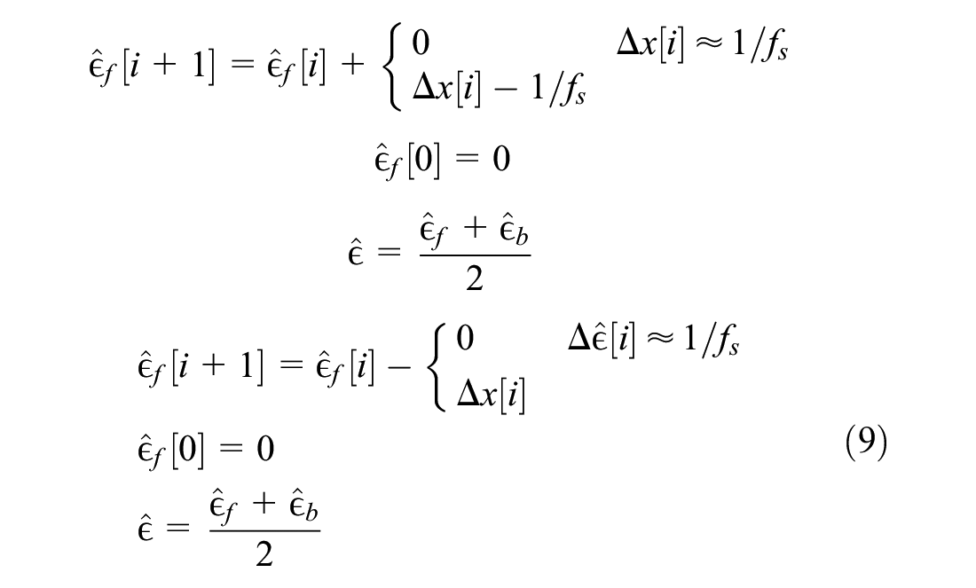
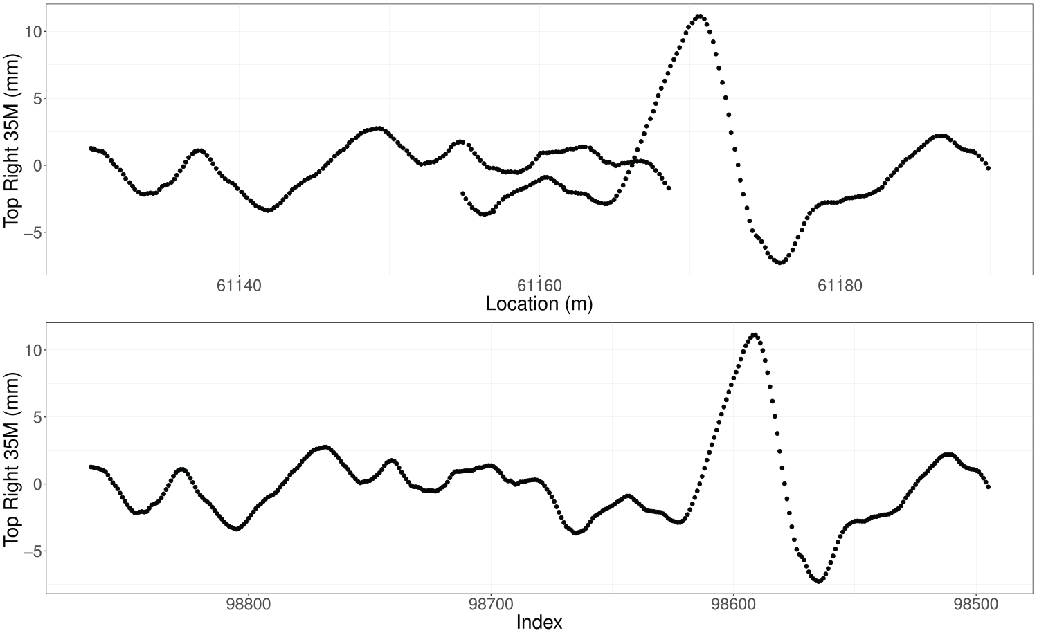
Since the the operation is symmetric, the average error is $\bar{ϵ} = 0$ . In subsequent sections we assume that a sample x has no position resets.

Figure 2.

Non-monotonic locations. Upper panel: Signal by location. Lower panel: Signal by index.

Convergence to True Location

Repeated samples $(x_{1}, y_{1}), (x_{2}, y_{2}), \dots, (x_{\infty}, y_{\infty})$ are independent. According to the law of large numbers ( 21 ), the average spatial error signal $ϵ$ tends to $0$ for any given location $\hat{x}$ as the number of independent sample signals increases.

\frac{1}{n} \sum_{i}^{n} {\hat{ϵ}}_{i} (\hat{x}) = 0

(10)

Drift

Consecutive measurements in a given sample $x_{k} [0], x_{k} [1], x_{k} [\dots]$ are, however, not independent. Their spatial errors ${\hat{ϵ}}_{k} [i]$ are strongly correlated and create a band-limited signal that drifts slowly (Inequality 11) and smoothly with an upper frequency bound $f_{d}$ (Inequality 12). Further we assume an absolute upper bound on the largest drift possible (Inequality 13).

| \frac{d}{d x} \hat{ϵ} (x) | << 1

(11)

f_{d} << f_{s}

(12)

| \hat{ϵ} | < T_{d}

(13)

These restrictions let us start with a coarse local alignment of the samples based on the largest drift possible (Inequality 13) and refine details (Inequality 12) with increasingly local (Inequality 11) alignment steps.

A drift that changes with frequency f and amplitude a will oscillate from $- a$ to a over the distance $1 / 2 f$ . A local alignment window thus needs to be shorter than $1 / 2 f$ to detect a drift of frequency f. Inequality 11 ensures that larger changes in drift have lower frequencies. Higher frequency drifts can be found in small local windows; that is, it is not necessary to search for potential drifts further away in other signals than the length of the alignment window.

Cross Correlation

The offset between two signals is found through cross correlation, a standard signal processing technique to search for similarity between signals which has been used extensively in various fields ( 22 , 23 ). Some examples from a wide variety of topics are high-speed sampling oscilloscopes ( 24 ), DNA sequence alignment ( 25 ), identifying street poles from images ( 26 ), and alignment of cosmic waves ( 27 ).

For continuous signals f and g, the cross correlation is defined as:

(f ★ g) (τ) \overset{Δ}{=} \int_{- \infty}^{\infty} \bar{f (t)} g (t + τ) dt

(14)

where $\bar{f (t)}$ is defined as the complex conjugate of $f (t)$ and $τ$ is the displacement or lag of the signals; that is, a feature in f at t occurs in g at $t + τ$ .

For signals measured at discrete points f and g, the cross correlation is defined as:

(f ★ g) [n] \overset{Δ}{=} \sum_{m = - \infty}^{\infty} \bar{f [m]} g [m + n]

(15)

where $\bar{f [m]}$ is defined as the complex conjugate of $f [m]$ and n is the displacement or lag of the signals; that is, a feature in f at m occurs in g at $m + n$ .

Alignment

An iteration of alignment starts by reconstructing an estimated signal. Let $y (x)$ denote a continuous signal reconstructed from spatially error-corrected measurements:

y (x [i] - e_{j}) = y [i]

(16)

The reconstructed signal is undefined for all x where the nearest sampled observation is further away than $T_{g}$ . Reconstructed signals are then pairwise compared using local cross correlations to find relative offsets. Let $o_{u, v} [i]$ denote the estimated relative offset between two signals u and v at window $W [i]$ .

o_{u, v} [i] = \arg max_{τ} (W_{i} {\hat{y}}_{u} ★ W_{i} {\hat{y}}_{v}) (τ)

(17)

A discrete approximation of this function uses a sample rate $f_{s}$ for the function $y (x)$ and interpolates the maximum of the cross correlation with a two-degree polynomial at the discrete $\arg max$ and its two neighbors.

o is undefined if the maximum correlation is less than a pre-defined threshold $T_{ρ}$ , or if either of $y_{u}$ or $y_{v}$ is undefined within the window. For each o let d be the distance to the nearest defined offset, with $d = 0$ if the corresponding offset o is defined.

Imputation

Let $\overset{\cdot}{o}$ be an imputed offset that interpolates from nearby windows where o is undefined. $\overset{\cdot}{o}$ has a corresponding weight $w = \max (0, 1 - d / T_{d})$ . Let the ( $j + 1$ )th estimated drift error be the weighted mean of the relative offsets:

{\hat{ϵ}}_{u}^{j + 1} = {\hat{ϵ}}_{u}^{j} + \frac{\sum_{v} {\overset{\cdot}{o}}_{u, v}^{j} w_{u, v}^{j}}{2 \sum_{v} w_{u, v}^{j}}

(18)

with ${\hat{ϵ}}_{u}^{j + 1} = 0$ if $\sum_{v} w_{u, v}^{j} = 0$ . ${\hat{ϵ}}_{u} = {\hat{ϵ}}_{u}^{J}$ denotes the estimated location error for measurement u. The aligned signals are then reconstructed from $y - γ = \hat{y} (\hat{x}) = \hat{y} (x - \hat{ϵ})$ .

Refinement of Spatial Error Estimate

The refined spatial error $ϵ$ can then be estimated for each sample by imposing that a weighted average within each window should still be 0 (Equation 10), where the weight depends on the distance from the nearest estimated relative offset. For windows without any relative offsets, we interpolate from the nearest relative offsets. At the edges, we extrapolate the first and last value.

r [i] = \frac{\sum_{j, k} {\hat{ϵ}}_{j, k} [i] w_{j, k} [i]}{\sum_{j_{k}} w_{j, k} [i]}

(19)

\hat{ϵ} [i] = (\sum_{j, j} o_{j, k} [i] - r_{w}) / 2

(20)

{\hat{\hat{ϵ}}}_{j} = {\hat{ϵ}}_{j} + \hat{ϵ} [i]

(21)

The refined spatial errors are estimated through iterating with half the window size until the window is small enough to capture the fastest changes in drift that are of interest (Inequality 11).

Results

Case Study

The visual alignment is how the end user perceives the performance of the algorithm. Figure 3 shows an alignment of a track geometry parameter where multiple window sizes are needed to mutually align the signals. QueryFileDate represents the date of the track measurement in the format yyyymmdd. Measurement running 20170526 to 20190114 have a drift of approximately 15 m, but the locations of the measurements from 20190211 drift approximately 60 m from the other runs.

Figure 3.

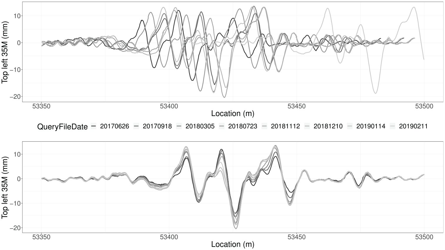
Example of drift where different window sizes are needed for mutual alignment. Upper panel: Signal before alignment. Lower panel: Signal after alignment.

Figure 4 shows the estimated spatial error signal for the alignment shown in Figure 3. The offsets for the different measurement runs differ between 5 and 60 m. Figure 5 shows an example of algorithm performance when the measurements of a track geometry parameter have a heterogeneous behavior, possibly because of maintenance activities. Measurements from 20170821 to 20180528 are well aligned, while another group of measurements from 20180625 to 20190701 show a different behavior. A possibly incorrect signal, measured on 20190311, is not well aligned to either of the groups. In the lower panel of Figure 5, showing the measurements before alignment, it is almost impossible to distinguish different signal behaviors.

Figure 4.

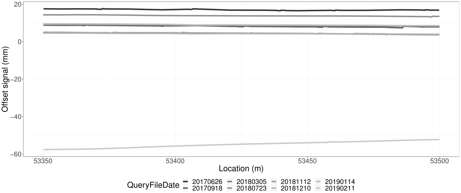
Estimated spatial error signals corresponding to Figure 3.

Figure 5.

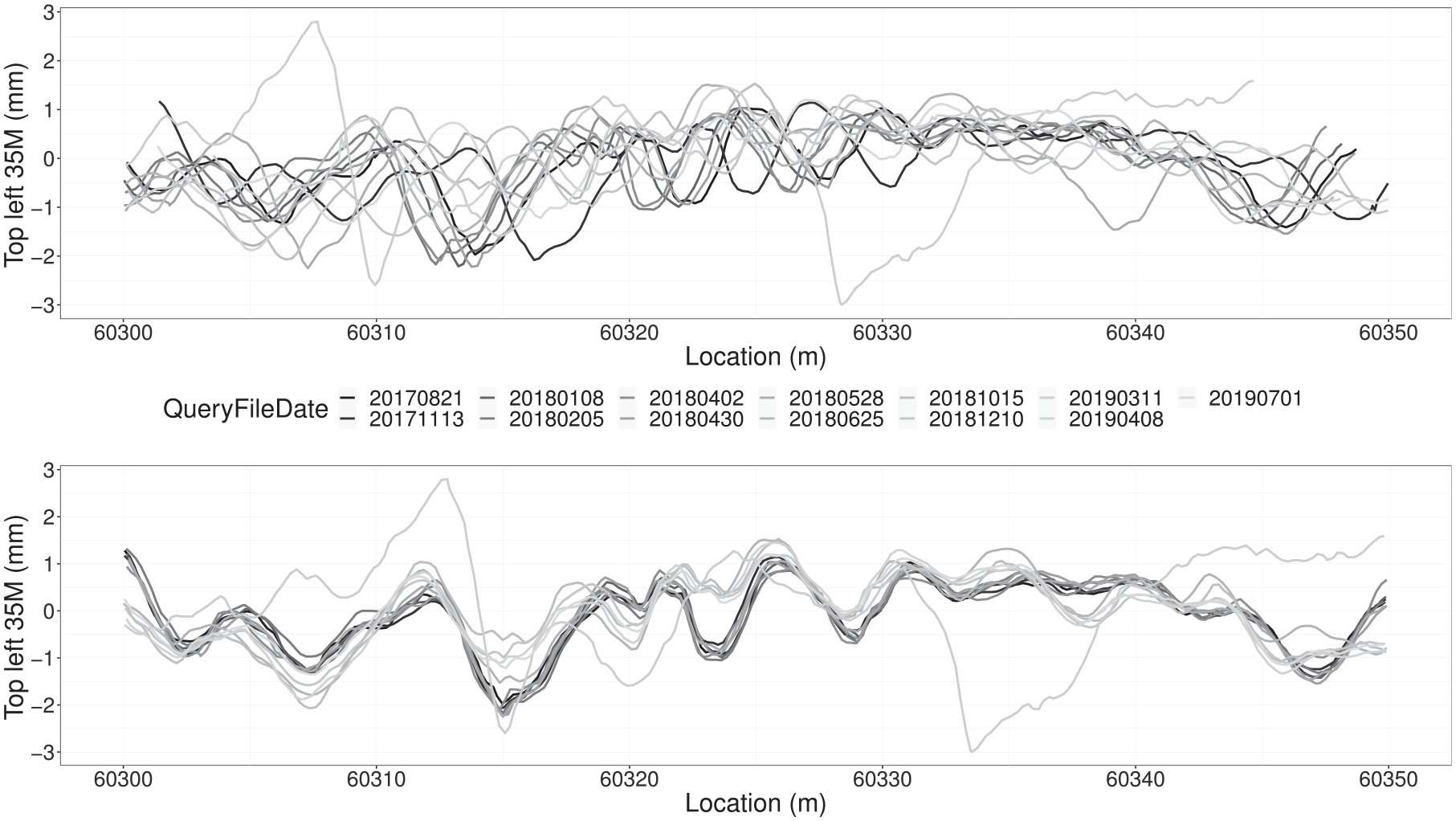
Example of signal with two different aligned groups, and one erratic signal QueryFileDate 20190311. Upper panel: Signal before alignment. Lower panel: Signal after alignment.

Discussion

Five challenging and previously unresolved aspects of mutually aligning track geometry signal data were stated in the Introduction: segmented data, variable sample rate, measurement errors, convergence to true locations, and consistency. This section discusses how our algorithm addresses each one of them.

Aligning Segmented Data

Aligning signals with cross correlation requires evenly sampled signals, equal in length. As shown in the section on Materials and Methods, measurement runs can range from 2,000 up to 47,000 m in length and not all runs may overlap.

By splitting each measurement run into continuous pieces, local cross correlation can be used to calculate the offset between pairwise continuous windows of two signals. For windows where the offset is undefined, that is, segments with no continuous overlap between signals, imputed offsets interpolated from nearby windows ensure that the estimated spatial error signal is continuous.

As highlighted in previous literature, it is critical to prove that mutual alignment works on realistic, empirical railway infrastructure data ( 17 ). Because measurement runs often differ in length and there may not be overlap between runs, an algorithm for mutual alignment must address this issue to be useful in practice. Our proposed algorithm successfully aligns segmented, empirical data with a very high precision in the alignment.

Variable Sample Rate

As described in section on Materials and Methods, the sample rate of the track geometry parameters measured by a tachometer is 200 mm. However, the GPS does not match the locations exactly to the tachometer sample rate. This mismatch must be adjusted to allow mutual alignment between signals.

Location resets in the RTPS causing mismatches between the track geometry parameter and locations are handled by creating an estimated location without resets. With resets removed, an accurate representation of the signal with one location per track geometry measurement point is achieved.

Measurement Errors

Our algorithm identifies spatial gaps in the sample signal and splits the signal into continuous pieces accordingly. Imputation of offsets (as described in the subsection Imputation) ensures that the signal is spatially correlated over the entire measurement run, despite the gaps.

The drift between measurement runs, that is, the spatially correlated measurement errors, is adjusted using an incremental reduction of local cross correlation windows. As seen in Figure 3, the drift varies vastly between different runs. At the same time, the precision of the alignment needs to be high enough to identify deterioration in the track geometry parameters. By iterating the algorithm using smaller cross correlation windows until sufficient granularity of the alignment is achieved (Figure 1), the proposed algorithm can mutually align signals with large drifts as well as obtain any desired level of precision.

Measurement errors in the track geometry parameters are not addressed by the algorithm. However, as can be seen in Figure 5, the alignment allows for erratic or incorrect signals to be identified. If the pre-defined correlation threshold is not met (see the section on Alignment), the offset of the estimated spatial error for that window is imputed from the nearest neighboring window. This procedure ensures that signals suffering from large measurement errors in the track geometry parameters will not affect the accuracy of the mutual alignment, and inaccurate measurements are more easily distinguished from accurate measurements.

Convergence

Through the law of large numbers, the mean of the estimated spatial errors will converge to zero, which ensures that the adjusted locations converge to the true locations. Previous literature concludes that monitoring deterioration of an exact location is not a prerequisite for effective maintenance ( 19 ). Although not crucial, convergence is a very attractive feature of the algorithm. It provides a reliable, stable estimate of the true location, reducing the need for other accuracy checks such as map matching.

Consistency

The railway track undergoes regular maintenance activities which are reflected in the measurements of the track geometry parameters. A static alignment algorithm, that is, aligning signals to a fixed reference, will inevitably cause inconsistencies when maintenance actions change the geometry of the track.

To achieve an alignment that is consistent over time, the algorithm must be able to update the alignment dynamically. When the track geometry parameters change because of maintenance, a new series of mutually aligned signals will occur, as seen in Figure 5.

Our algorithm attains consistency through two different steps. First, it imposes a threshold of each local cross correlation. This ensures that when the signal of a track geometry parameter changes characteristic because of maintenance, it is mutually aligned with other signals exhibiting a similar pattern. Second, the refinement of the estimated spatial error ensures that different groups of mutually aligned signals have an accurate location. By setting the sum of a weighted average over all windows to zero (as described in the section Refinement of Spatial Error Estimate), the estimated locations are consistent over time despite maintenance activities taking place.

In a production setting, consistency is maintained by running the alignment algorithm each time a new measurement run is added to the database.

Limitations

The law of large numbers implies that a sufficient amount of data must be aligned to ensure convergence. With only a few measurement runs, convergence to true locations cannot be guaranteed. The algorithm does not use fixed reference points, which is an advantage in terms of flexibility. However, in certain practical applications, for example, when compiling several geospatial data sources, fixed references might sometimes be required. This can be achieved by fixing the algorithm at a specific alignment, but by doing so, the algorithm does no longer converge to true locations as more data is added.

Conclusion

Condition monitoring is a crucial aspects for railway safety as well as efficient maintenance planning. The novel algorithm for mutual alignment of track geometry data presented in this paper addresses five key features which must be resolved to enable monitoring of deterioration over time as well as predictive maintenance. The algorithm successfully solves alignment of segmented data sampled at variable sample rates, spatially correlated and uncorrelated measurement errors, convergence to true locations, and consistent alignment over time. The limitations of the algorithm mainly apply to the amount of data and flexibility in the alignment required to ensure convergence. The advantages of the algorithm are shown in a case study by aligning nine different track geometry parameters on a reference line operated by British Network Rail.

Footnotes

Acknowledgements

The authors wish to acknowledge the support from Network Rail for releasing the algorithm to public knowledge. Special thanks to Jonathan Schofield for proofreading and insights, and Russell Licence for providing knowledge about the positioning systems on Network Rail’s measurement trains. Three anonymous reviewers contributed to improve the quality of this paper.

Author Contributions

Authors have contributed as follows: conceptualization: K. Eklöf and A. Nwichi-Holdsworth; methodology: K. Eklöf and J. Eklöf; validation: J. Eklöf; formal analysis: K. Eklöf; investigation: A. Nwichi-Holdsworth; resources: A. Nwichi-Holdsworth; data curation: K. Eklöf; writing—original draft preparation: K. Eklöf; writing—review and editing: K. Eklöf; visualization: K. Eklöf.

Declaration of Conflicting Interests

The author(s) declared no potential conflicts of interest with respect to the research, authorship, and/or publication of this article.

Funding

The author(s) received no financial support for the research, authorship, and/or publication of this article.

ORCID iD

Kristin Eklöf

References

Ebersöhn

Selig

E. T.

Use of Track Geometry Measurements for Maintenance Planning. Transportation Research Record: Journal of the Transportation Research Board, 1994. 1470: 84–92.

Hyslip

J. P.

Fractal Analysis of Track Geometry Data. Transportation Research Record: Journal of the Transportation Research Board, 2002. 1785(1): 50–57.

Sadeghi

Development of Railway Track Geometry Indexes Based on Statistical Distribution of Geometry Data. Journal of Transportation Engineering, Vol. 136, No. 8, 2010, pp. 693–700.

Choi

Chung

Kim

H.-Y.

Park

Yoon

Replacement Condition Detection of Railway Point Machines Using an Electric Current Sensor. Sensors, Vol. 17, No. 2, 2017, p. 263.

Wei

Núñez

Dollevoet

Evaluating Degradation at Railway Crossings Using Axle Box Acceleration Measurements. Sensors, Vol. 17, No. 10, 2017, p. 2236.

Gabara

Sawicki

A New Approach for Inspection of Selected Geometric Parameters of a Railway Track Using Image-Based Point Clouds. Sensors, Vol. 18, No. 3, 2018, p. 791.

Lin

Zhang

Ding

Faults Diagnostics of Railway Axle Bearings Based on IMF’s Confidence Index Algorithm for Ensemble EMD. Sensors, Vol. 15, No. 5, 2015, pp. 10991–11011.

Yang

Tao

Liu

Zhang

Zhao

An Efficient Direction Field-Based Method for the Detection of Fasteners on High-Speed Railways. Sensors, Vol. 11, No. 8, 2011, pp. 7364–7381.

Martey

E. N.

Ahmed

Attoh-Okine

Track Geometry Big Data Analysis: A Machine Learning Approach. Proc., 2017 IEEE International Conference on Big Data (Big Data). IEEE, 2017, pp. 3800–3809.

10.

Jiang

A New Filtering and Smoothing Algorithm for Railway Track Surveying Based on Landmark and IMU/Odometer. Sensors, Vol. 17, No. 6, 2017, p. 1438.

11.

Weston

Roberts

Yeo

Stewart

Perspectives on Railway Track Geometry Condition Monitoring from In-Service Railway Vehicles. Vehicle System Dynamics, Vol. 53, No. 7, 2015, pp. 1063–1091.

12.

Karaim

Elsheikh

Noureldin

Rustamov

GNSS Error Sources. In Multifunctional Operation and Application of GPS ( Rustamov

R. B.

Hashimov

A. M.

, eds.), IntechOpen, London, 2018, pp. 69–85.

13.

Chen

Niu

Zhang

Cheng

Railway Track Irregularity Measuring by GNSS/INS Integration. Navigation: Journal of the Institute of Navigation, Vol. 62, No. 1, 2015, pp. 83–93.

14.

Reimer

Müller

Hinüber

INS/GNSS/Odometer Data Fusion in Railway Applications. Proc., 2016 DGON Inertial Sensors and Systems (ISS). IEEE, 2016, pp. 1–14.

15.

Saab

S. S.

A Map Matching Approach for Train Positioning. I. Development and Analysis. IEEE Transactions on Vehicular Technology, Vol. 49, No. 2, 2000, pp. 467–475.

16.

Saab

S. S.

A Map Matching Approach for Train Positioning. II. Application and Experimentation. IEEE Transactions on Vehicular Technology, Vol. 49, No. 2, 2000, pp. 476–484.

17.

Al-Douri

Y. K.

Tretten

A Critical Review of Information Assurance (IA) Framework for Condition-Based Maintenance of Railway Tracks. In European Safety and Reliability Conference (ESREL 2016), Glasgow, 25/09/2016-29/09/2016. CRC Press, 2017, pp. 1072–1078.

18.

Faiz

R. B.

Edirisinghe

Singh

An Empirical Rail Track Degradation Model Based on Predictive Analysis of Rail Profile and Track Geometry. PhD thesis. Loughborough University, 2010.

19.

Bergquist

Söderholm

Kauppila

Vanhatalo

Cleaning of Railway Track Measurement Data for Better Maintenance Decisions. Proc., 5th International Workshop and Congress on eMaintenance. 2019, p. 9.

20.

Lewis

Track Geometry Recording and Usage at Network Rail. Network Rail, Derby, 2008.

21.

Dekking

F. M.

Kraaikamp

Lopuhaä

H. P.

Meester

L. E.

A Modern Introduction to Probability and Statistics: Understanding Why and How. Springer Science & Business Media, 2005.

22.

Bracewell

Pentagram Notation for Cross Correlation. The Fourier Transform and Its Applications. McGraw-Hill, New York, Vol. 46, 1965, p. 243.

23.

Rabiner

L. R.

Schafer

R. W.

Theory and Applications of Digital Speech Processing, Vol. 64. Pearson Upper Saddle River, NJ, 2011.

24.

Coakley

K. J.

Hale

Alignment of Noisy Signals. IEEE Transactions on Instrumentation and Measurement, Vol. 50, No. 1, 2001, pp. 141–149.

25.

Rockwood

A. L.

Crockett

D. K.

Oliphant

J. R.

Elenitoba-Johnson

K. S.

Sequence Alignment by Cross-Correlation. Journal of Biomolecular Techniques: JBT, Vol. 16, No. 4, 2005, p. 453.

26.

Abdalla

Easa

S. M.

Extracting Streetlight Poles from Orthophotos: Methodology and Case Study in Ontario, Canada. Journal of Surveying Engineering, Vol. 133, No. 4, 2007, pp. 184–187.

27.

Troxel

Ishak

Cross-Correlation between Cosmic Microwave Background Lensing and Galaxy Intrinsic Alignment as a Contaminant to Gravitational Lensing Cross-Correlated Probes of the Universe. Physical Review D, Vol. 89, No. 6, 2014, p. 063528.