
Abstract
We propose a new methodology for calibrating Wiedemann-99 vehicle-following parameters for mixed traffic (different conventional vehicle classes) based on trajectory data. The existing acceleration equations of the Wiedemann model are modified to represent more realistic driving behavior. Exploratory analysis of simulation data revealed that different Wiedemann-99 model parameters could lead to similar macroscopic behavior, highlighting the importance of calibration at the microscopic level. Therefore, the proposed methodology is based on optimizing performance measures at the microscopic level (acceleration, speed, and trajectory profiles) to estimate suitable calibration parameters. Further, the goodness of fit for the observed data is sensitive to the numerical integration method used to compute vehicles’ velocity and position. We found that the calibrated parameters using the proposed methodology perform better than other approaches for calibrating mixed traffic. The results reveal that the calibrated parameter values and, consequently, the thresholds that delineate closing, following, emergency braking, and opening regimes, vary between two-wheelers and cars. The window (in the relative speed versus gap plot) for the unconscious following is larger for cars while the free-flow regime is more extensive for two-wheelers. Moreover, under the same relative speed and gap stimulus, two-wheelers and cars may be in different regimes and display different acceleration responses. Thus, accurate calibration of each vehicle’s parameters is essential for developing micro-simulation models for mixed traffic. The calibration analysis results of strict and overlapping staggered car following signify an impact of staggered car following compared with strict car following which demands separate calibration for strict and staggered following.
Microscopic traffic flow models represent traffic in greater detail and generate more performance measures than macroscopic or mesoscopic models. They enable the evaluation of a wide range of traffic interventions and scenarios before implementation. Moreover, they reflect the dynamic and random nature of the transportation system ( 1 ). They are, therefore, robust and cost-efficient tools for modeling them.
A microscopic traffic flow model consists of sub-models that describe human driver behavior such as gap acceptance, speed adaptation, lane changing, ramp merging, overtaking, and car following. The latter, on which we focus here, describes the interactions with preceding vehicles in the same lane including the special case of free flow with no interactions ( 2 ).
One of the critical elements of using microscopic models is calibration. The value of the simulation models’ various parameters is determined to match the observed real traffic behavior. As no single traffic model can represent all traffic conditions, every model must be adapted to local needs using real-world data. Parameter calibration in simulation applications is, therefore, critical to replicate driving behavior in the field. This study focuses on calibrating a widely used psychophysical vehicle-following model (Wiedemann-99 [W-99] model) for India’s mixed traffic conditions using vehicle trajectory data.
The W-99 ( 3 ) model has been widely used in traffic micro-simulation for both lane-based and non-lane-based conditions (1, 4–12). However, this model’s use in non-lane-based states will be substantially different from lane-based conditions and requires careful calibration. These differences arise, in particular, from the presence and composition of additional vehicle types such as two-wheelers or auto-rickshaws, different static and dynamic characteristics of vehicles, and a lack of strict lane discipline. As a result, vehicles are free to occupy any available lateral position on the road space. Moreover, smaller vehicles (two-wheelers) often use gaps between larger vehicles in the traffic stream ( 13 ). Another critical aspect of the non-lane-based mixed traffic condition is the possible difference in the following behavior when the subject vehicle is strictly behind a leading vehicle versus when it is overlapping and staggered compared with the vehicle ahead ( 14 ).
A recently proposed model for lane-free mixed traffic ( 15 ) provides a generalized framework for extending conventional car-following models (including the Wiedemann car-following model) to a fully 2-D microscopic model. In the presence of multiple leaders and staggered following, this framework assumes, with good results, that the longitudinal dynamics depend only on the leader with the strongest interaction and that the repulsive force remains unchanged as long as there is a lateral overlap, that is, the longitudinal acceleration reverts to that of the underlying car-following model. One goal of the present analysis is to test this assumption by distinguishing between the strict and staggered following.
The key feature for calibration of mixed traffic conditions is the response of the driver of a subject vehicle to the vehicles present in the neighborhood and their maneuvers. One should note that the model parameters may vary based on leader, follower, and surrounding vehicle types and their speeds and positions ( 16 ). There is a growing body of work on the calibration of various microscopic models for mixed traffic using multiple models (5, 6, 8–13, 16–20). The analytical forms of some of the Wiedemann model equations are not easily accessible in the literature, making the calibration at the trajectory level difficult. As a result, very few of these studies attempted to analyze the errors entailed in the calibration process of a Wiedemann model and its impact on the accuracy of results at the trajectory level ( 21 ).
In light of the above motivations and gaps in the literature, this paper has the following objectives.
propose and implement an optimization-based procedure for calibrating the W-99 model vehicle-following parameters using trajectory data of mixed traffic;
propose modifications of the acceleration equations to represent more realistic driving behavior;
evaluate alternative numerical integration methods for prediction of speed and position at the trajectory level;
evaluate the proposed calibration with other calibration methods reported in the literature;
analyze differences in the vehicle-following behavior of two-wheelers and cars in mixed traffic; and
investigate differences in parameters between “strict” and “overlapping” following situations for selected vehicle types.
The paper is organized as follows. The next section provides a brief review of the W-99 model and a synthesis of the literature with this study’s objectives. The rationale for calibration of the W-99 model using trajectory data is then presented. This is followed by a description of the data and the calibration methodology. The salient results and findings are discussed before the conclusion.
Literature Review
The W-99 model is presented first, followed by a synthesis of the literature on the calibration of car-following models.
Wiedemann Car-Following Model
As a psychophysical model, the W-99 model ( 3 ) uses thresholds or action points, where the driver changes behavior at discrete time points. Drivers change their response to the local situation (gap, speed, or relative speed) only when these thresholds are reached ( 2 ). This model’s concept is that faster moving drivers approaching slower vehicles start decelerating when they reach their perception threshold. However, because of imperfections in estimating speeds, the speed may become smaller than that of the leader. So, the driver may accelerate slightly again after reaching another threshold ( 7 ). The combined effect of the thresholds and estimation errors leads to a hysteresis when plotting the trajectory in the space given by the relative speed and the gap. Wiedemann ( 22 ) defined the relative speed between the lead and following vehicles as the stimulus, which triggers the following vehicle’s reaction. Using different perception thresholds, four different driving regimes were proposed.
In the free-flow regime, the subject vehicle is not influenced by any other leader; the driver tries to maintain the desired speed and uses a speed-dependent maximum acceleration to reach the desired speed.
In the closing-in regime, the driver has perceived a slower leader and continuously decelerates till the speed matches the leader’s speed (the relative speed becomes zero), and the gap equals the desired gap. Then, the driver enters the following regime.
In the following regime, the driver of the subject vehicle unconsciously follows the leader trying to maintain an ideal gap and zero relative speed using comparatively low accelerations or decelerations.
In the emergency braking regime, if the following distance falls below a critical threshold, the driver reacts by applying the maximum deceleration (within vehicular capabilities) to avoid a potential collision.
Figure 1 shows the boundaries of these regimes, which are defined by following six different perceptual thresholds:
AX: the desired distance between two vehicles in a stopped condition;
ABX: the desired minimum safe following distance in moving state, as a lower limit of the following regime;
SDX: the maximum following distance as the upper limit of the following regime;
SDV: the points at long distances (more than SDX) where drivers perceive that they are approaching slower vehicles;
CLDV: the points at short distances (less than SDX) where drivers perceive that their speeds are higher than their lead vehicle speeds; and
OPDV: the points at short distances (less than SDX) where drivers perceive that they are traveling slower than their leader.
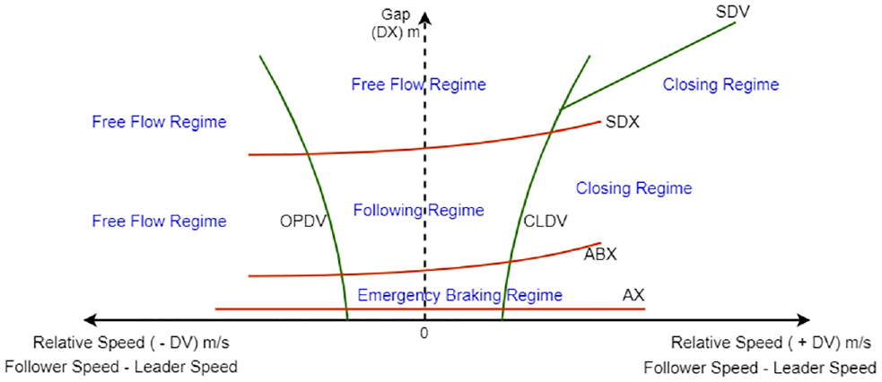
Schematic representation of Wiedemann model ( 22 ).
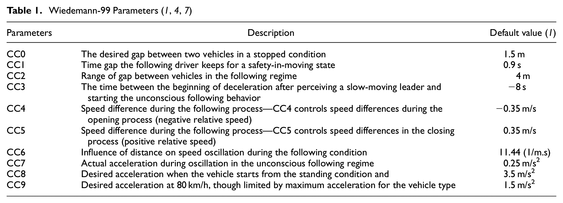
The W-99 model ( 3 ) is calibrated using the driving behavior parameters (CC parameters); these parameters are defined based on regime classification thresholds. The description and the default values of the CC parameters are given in Table 1.
Calibration of Wiedemann Car-Following Models in Heterogeneous Traffic
Many studies ( 1 , 4 , 7 , 23 ) have calibrated the Wiedemann parameters for homogeneous traffic flow data. Some have calibrated a single parameter set for all vehicle classes. In most studies (8–12, 17, 18) calibration procedures are based on matching the macroscopic performance measures from a simulation package (e.g., VISSIM) such as flow, density, speed, or delays with field data, primarily because of data limitations of cross-sectional video measurements. Other studies ( 24 – 26 ) used test track data or synthetic data to calibrate the vehicle-following models and, therefore, the applicability of the parameters to real-world traffic is unclear.
While trajectory data have been used to calibrate other vehicle-following models such as the Gipps model ( 27 ) or the IDM ( 28 ), presumably as a result of the more straightforward equations involved, very few studies ( 23 ) focus on calibrating Wiedemann car-following models using trajectory data based on microscopic performance measures such as the speed profiles of individual vehicles. This lack of research is attributable partly to limitations of the data collected using location-based sensors, which give measurements at only selected cross-sections.
On the issue of mixed traffic, a growing number of studies have investigated the calibration of various vehicle-following models such as Krauss ( 29 ), Gipps ( 27 ), IDM ( 28 ), and W-99 ( 3 ). Again, the majority are based on macroscopic measures of performance. The mixed traffic flow model (MTM) is proposed as a generalized framework for car following ( 15 ). A few other studies ( 13 , 16 , 19 , 20 ) aim to calibrate other models, such as Gipps’s model and the IDM using field data. Still, they do not explicitly capture the differences in driving behaviors across regimes (following, closing, emergency braking, opening, and free flow) sufficiently. Very few studies ( 6 , 7 ) have used microscopic trajectory data for calibrating W-99 models in mixed traffic but use heuristic or data-driven procedures to estimate vehicle-following parameters. Two essential concerns with these procedures include: the parameter estimates are not directly linked to differences between observed and computed trajectories at the microscopic level (position, speed, acceleration profiles of individual vehicles over time), and the quality of the resulting parameters is difficult to assess. Thus, there is a need to use optimization-based procedures to calibrate psychophysical models for mixed traffic using trajectory data. This will enable the evaluation of the effect of the model parameters on the deviation between observed and estimated speed, acceleration, and position profiles. Furthermore, in the context of mixed traffic, there is a need to understand whether, and to what extent, the W-99 parameters vary with the vehicle type (two-wheelers, cars, etc.) Another question is whether the parameter values found by trajectory calibration are comparable to those found with macroscopic calibration Finally, the influence of the kind of following (strict and staggered), specifically regime thresholds, also needs investigation in the context of the W-99 model.
In light of the above gaps, this study focuses on the W-99 car-following model’s calibration using real-world trajectory data under heterogeneous and non-lane-based (mixed traffic) conditions. In this study, the W-99 model’s acceleration equations are used for trajectory estimation rather than VISSIM generated data. W-99 parameters are calibrated by microscopic criteria such as the deviation between observed and estimated speed, acceleration, and position profiles at a microscopic level in mixed traffic data.
Rationale for Calibrating the W-99 Model Using Trajectory Data
This section analyzes the effect of different sets of microscopic vehicle-following parameters for mixed traffic on the resulting macroscopic traffic flow performance measures (average speed, flow, densities).
A study stretch (245 m) on a three-lane midblock section (described below) is considered for this analysis. Three different sets of the calibrated parameter values are input into the VISSIM traffic simulation software and macroscopic and microscopic measures (vehicle level position, speed, and acceleration profiles) are obtained for each set. Parameter sets 1, 2, and 3 (cf. Figure 2) are obtained by applying heuristics based on macroscopic criteria as reported in the literature ( 6 , 7 , 30 ). The vehicular composition and vehicle dimensions (average length and width of each vehicle class) are taken from Kanagaraj et al. ( 31 ). Kinematic parameters (maximum acceleration/deceleration, desired acceleration/deceleration, free-flow speed) are taken from Arasan and Koshy ( 32 ), Asaithambi et al. ( 17 ), and Kashyap et al. ( 14 ). The differences in the CC parameters and associated threshold values across the sets are depicted in Figure 2 (for a constant leader speed of 10 m/s).
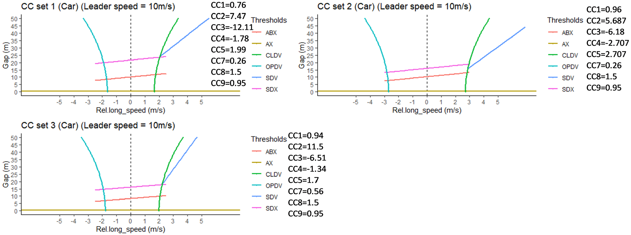
Wiedemann thresholds plots for different sets of driving behavior (CC) parameters.
The simulation model is run for a study period of 30 min for 100 different random seeds for a given set of Wiedemann parameters. The volume, density, and average speed for each vehicle class are calculated, and the procedure is repeated for different sets of Wiedemann parameters.
A set of pair-wise t-tests are performed for equal means of speed and density. In all sets, the equality of mean speed cannot be rejected (p-values were 0.2, 0.36, and 0.16 for CC set 1 and CC set 2, CC set 1 and CC set 3, and CC set 2 and CC set 3, respectively). The mean densities are also not significantly different across the parameter sets (p-values were 0.58, 0.54, and 0.34, respectively, for the above pairs). Thus, the different CC parameter sets yield statistically similar macroscopic performance measures, despite the significant difference in microscopic behavior.
Trajectories of simulated data generated using the same input volume, speed, and acceleration distributions as explained above with the same random seed and different W-99 parameters (CC sets 1, 2, and 3) are plotted in Figure 3. These trajectories are for the same single lane and for the same time interval for all sets of W-99 parameters. The macroscopic measures such as average speed, density, and volume of 100 replications of each set of CC parameters for the three-lane study stretch (described below) are noted in the following plot. Major differences in the trajectories at the same time across different CC sets are marked with circles A, B, and C.
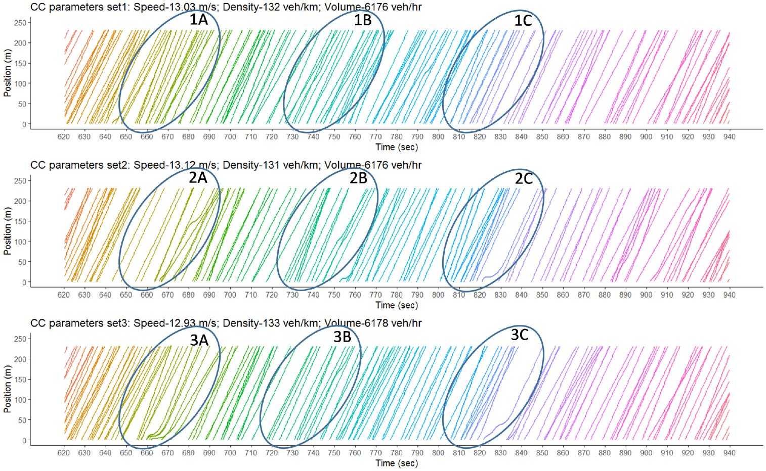
Trajectory plots of simulated data for different sets of driving behavior (CC) parameters.
From left-hand circles (A) of each trajectory plot, we can see that:
1A—trajectories are close to each other;
2A—trajectories are very scattered compared with 1A and 3A; and
3A—there is a difference in the slope of some trajectories as well as some vehicles with some delay at the start.
From central circles (B) of each trajectory plot, we can see that:
1B—trajectories are very close to each other and some vehicles are crossing the trajectories of other vehicles
2B—vehicles in the circle have varied speeds with some vehicles showing delay at time 750; and
3B—vehicles are scattered as compared with 1B and 2B.
From the right-hand circles (C) of each trajectory plot, we can see that:
1C—most vehicles are moving at the same speed as trajectories are parallel, some vehicles are crossing the trajectories of other vehicles;
2C—vehicles are very close to each other for time 810 to 820 and there is some lag in a vehicle starting at time 820; and
3C—vehicles are closer to each other than in 1C but not as close as in 2C. The lagged behavior of vehicles starting at 820 is different from 2C.
These results indicate that different CC parameters show significantly different microscopic behavior but result in similar macroscopic behavior. The CC parameters, therefore, need to be calibrated at a microscopic level to have consistency at that level.
Data Collection
Video data were collected from a six-lane divided urban arterial road at the Maraimalai Adigalar Bridge in Saidapet, Chennai, India by Kanagaraj et al. ( 31 ). The section selected (Figure 4) is a bridge with a uniform road width. There are no nearby intersections, bus stops, parked vehicles, or other forms or side friction that would affect driver behavior. Furthermore, there is no interaction between the vehicle traffic and pedestrians; the study section’s width is 11.2 m, and its length is 245 m.
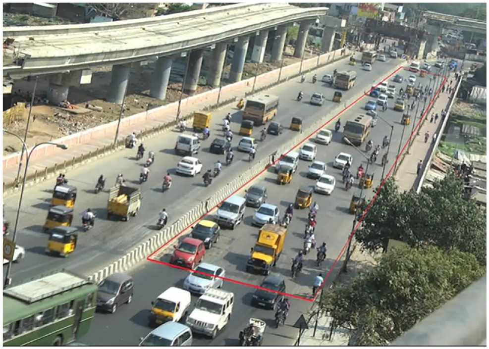
Photograph of the study section ( 31 ).
The coordinates, dimensions, and class of all vehicles in the video sequences for 30 min between 2:45 and 3:15 p.m. were obtained using a trajectory extractor. Data consists of a total of 3,016 vehicles of six different classes. Data were recorded at a resolution of 0.52 s ( 31 ).
Descriptive Statistics of Data
Traffic data consist of 1,703 (57%) motorized two-wheelers (TW); 802 (27%) Cars; 367 (12%) auto/three-wheelers (3W); 95 (3%) Buses; 40 (1%) light commercial vehicles (LCV); and 9 (0.29%) heavy commercial vehicles (HCV). The collected data set includes 3,016 vehicle trajectories with a total of 130,137 data points.
For the given data, vehicular trajectories are drawn as time-space plots. Figure 5 shows a sample of 82 trajectories of cars and 171 trajectories of two-wheelers for the same period. The vehicle trajectories have different slopes reflecting different speeds. Intersecting trajectories denote passing on either side. From both plots, we can see that there is different behavior of both vehicle classes; there is much variation in two-wheelers trajectory slopes while those of cars are comparatively steady. Furthermore, two-wheelers have other values for the desired speed, acceleration, and longitudinal gaps (Section 3). Two-wheelers and cars have, therefore, distinctively different longitudinal behavior.
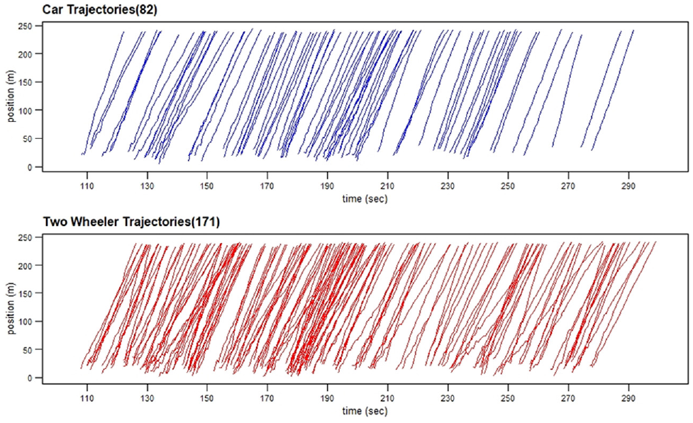
Trajectories plot.
Leader-Follower Pair Identification
The influence area method by Anand et al. ( 16 ) is selected to identify the tentative leader–follower pairs. Using this method, a total of 2,130 pairs are identified consisting of (1,056 TWs; 695 Cars; 280 3W; 62 Buses; and 37 LCVs) as subject vehicles.
Two features are essential in defining the following behavior. First, the follower can perceive the changes in the leader’s speed/acceleration or gap when the leading vehicle is within certain limits and responds by changing acceleration, speed, and position. Second, the following behavior must continue for a sufficient time duration.
Accordingly, the “actual” or “true” leader–follower pairs are identified based on the following criteria. The maximum longitudinal gap should be less than 30 m. No other vehicle should be present between an identified leader and follower. There must be lateral overlap between leader and follower. The following behavior (above three criteria) must be present for a duration of more than 5 s.
Pairs must show the hysteresis behavior, that is, oscillations of relative speed and the gap from the unconscious following behavior as defined in the Wiedemann model to capture the responsiveness of the follower to the lead vehicle, sample hysteresis plots of relative speed (X-axis) and gap (Y-axis) are shown in Figure 6. The vehicle pair in Figure 6a exhibits symmetric oscillations or hysteresis around the X-axis, in this regime; the follower tries to keep the same speed as the leader, that is, a relative speed near to zero, but the speed may become lesser/higher than that of the lead vehicle speed as a result of the driver’s imprecision in estimating the lead vehicle speed. So, the driver will accelerate/decelerate slightly again after reaching another threshold. This results in an iterative process of acceleration and deceleration leading to hysteresis because of the driver’s imprecision in determining the exact speed of the leader. The relative speed, therefore, oscillates near zero, which is shown in the hysteresis plot (Figure 6a).
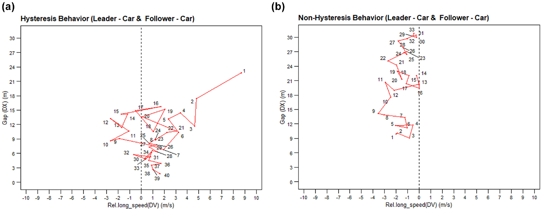
Gap-relative speed plots displaying: (a) hysteresis behavior; and (b) non-hysteresis behavior.
In contrast, as shown in Figure 6b which illustrates non-hysteresis behavior, there are no oscillations of the relative speed around zero in the following regime.
After applying the above conditions to the 2,130 tentative leader–follower pairs, a total of 1,236 (544 TWs; 480 Cars; 155 3Ws; 35 Buses; and 22 LCVs) pairs are identified as true leader–follower pairs. Among these, very few cases with multiple leaders are identified (63 out of 1,024 pairs). For the calibration and analysis, subsequently, multiple leaders are considered as separate leaders. The following response can be taken as the most conservative response of the subject vehicle to these leaders. For all the regimes in multiple leader cases, a conservative braking approach is considered, that is, for a data point, the smallest predicted acceleration by all leaders is considered.
Proposed Scheme for Calibrating W-99 Parameters Using Trajectory Data in Mixed Traffic
This section explains the optimization-based procedure for calibrating W-99 following parameters using vehicle trajectory data in mixed traffic. Figure 7 gives an overview of the calibration methodology.
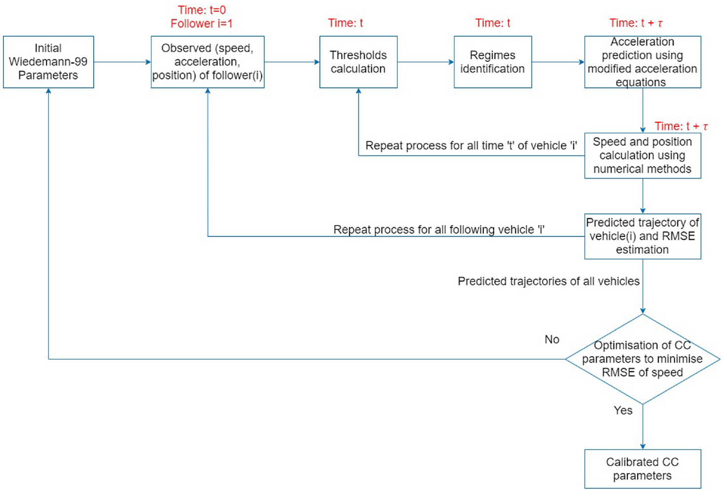
Calibration methodology.
For the assumed initial following parameters (CC), starting time t is set to t0 (the initial time when following begins).
Step 1: Perpetual Threshold (as defined in Section 2.1) computations are performed at time t.
Step 2: Based on thresholds in Step 1, regimes are identified at time t.
Step 3: Based on the regimes in Step 2, the acceleration is computed for the follower at time t + τ (where τ is reaction time) using modified equations given below.
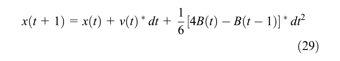
Step 4: Speed of the following vehicle is computed at time t + τ by numerical integration of accelerations in Step 3 using equations given below.
Step 5: The position of the following vehicle is determined at time t + τ by numerical integration of acceleration in Step 3 and speed in Step 4.
Step 6: The longitudinal gap and speed difference are updated for time t + τ based on Steps 4 and 5.
Step 7: The time step is incremented.
The above process is repeated to predict all points of the given vehicle and then predicted trajectories of all vehicles for the given set of following parameters.
The deviation between observed and predicted acceleration, speed, and position are computed using root mean squared error (RMSE) for all “actual” leader–follower pairs. The CC parameters are calibrated by optimizing the Wiedemann model with an objective function to minimize RMSE between observed and predicted speeds.
Regime Classification Procedure
The clear gap DX and relative speed (follower speed minus leader speed) DV are computed at time t, the driving regime of follower at time t is determined based on the following conditions as per Aghabayk et al. ( 1 ).
Case 1: IF [DX(t)>=SDX(t) & DV(t)<=SDV(t)] OR IF [DV(t) <OPDV(t)], then regime at time t is free flow regime.
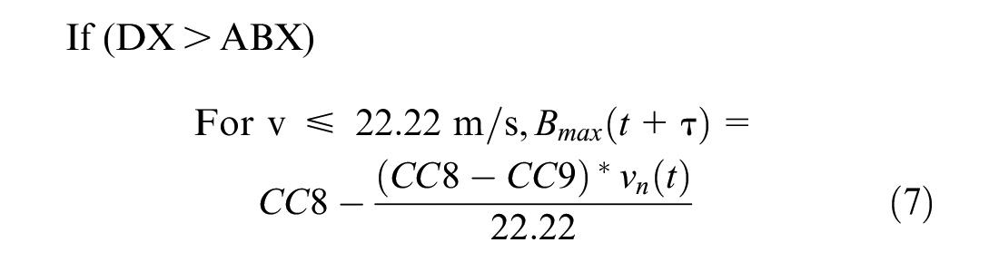
Case 2: IF [DX(t) > ABX(t) & DX(t) < SDX(t) & DV(t) > CLDV(t)] OR IF [DX(t) >=SDX(t) & DV(t) > SDV(t)], then the follower is in closing regime at time t.
Case 3: IF [DX(t) > ABX(t) & DX(t) < SDX(t) & DV(t) > OPDV(t) & DV(t)<=CLDV(t)] then regime at time t is following
Case 4: IF [DV(t) ≥ OPDV(t) & DX (t)≤ ABX(t) & DX(t) > AX(t)], then regime is emergency braking at time t
The threshold equations for the above regime classification are as follows:


The driving regime at time t is identified using the above conditions and thresholds, and for the identified regime, the acceleration is computed for the follower at time t + τ.
Modification in Wiedemann Acceleration Equations
The difficulties with existing acceleration equations in the literature and proposed modification are as follows:
i. Free-flow regime
The existing acceleration equation in the free-flow regime is

The existing acceleration equation assumes a constant free-flow speed of 22.22 m/s, but it is unrealistic to have the same free-flow speed for all vehicles and road conditions. Also, it assumes that acceleration will be non-negative (CC9) for a speed of more than 22.22 m/s, but the vehicle should decelerate at higher speeds.
The following equation is used to reflect two modifications:
Instead of the fixed free-flow speed of 22.22 m/s, vehicle and road type-specific free-flow speed from observed data is considered (using vmi, which is specific for vehicle type i).
The α value is set as 0.4, which ensures that at speeds higher than the road’s design speed, acceleration should be negative to achieve the design speed.
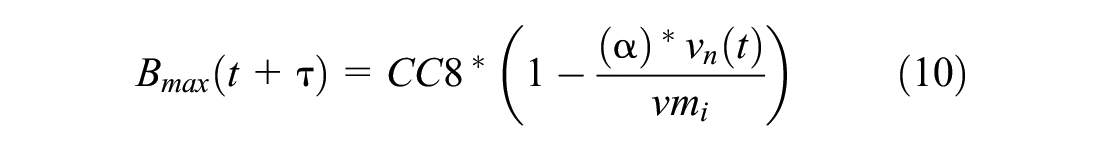
where vn(t) = current speed in m/s & vmi = free-flow speed for vehicle type i in m/s
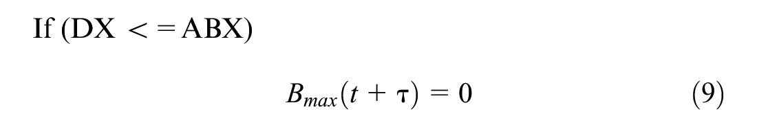
If (DX <=ABX)

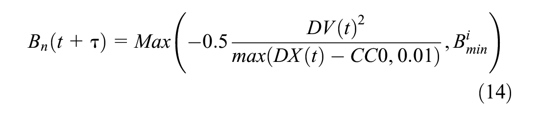
ii. Closing regime
The existing acceleration equation is

In the existing equation, when the gap (DX) is close to ABX, then the Bn value increases sharply and will be restricted to Bmin; this corresponds to an artificial and “virtually solid wall” at the transition between the following and the emergency braking regime. Also, by the equation of Bmin, it can have practically unachievable value at lower speeds.
To address these issues, the following modifications are suggested:
1. ABX in the denominator is replaced with CC0, which allows the driver to go closer to the leader than the original formula to match leader speed. This also means that the safety margin is reduced with respect to the original W-99 which is partially compensated for by the next modification. Moreover, we simulated the modification extensively and could not observe accidents.
2. The first term’s denominator is limited to values greater than 0.01 m to avoid zero denominators and discontinuous accelerations.
3. Bmin is treated as a vehicle-specific quantity for mixed traffic.
iii. Following regime
The existing acceleration equation is
In the existing acceleration equation, CC7 can take a value greater than Bmax, which is physically not possible. The modification proposed is:
If DV(t) < 0

If DV(t) >= 0

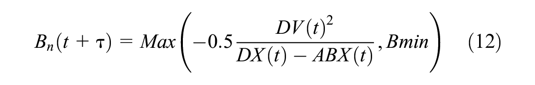
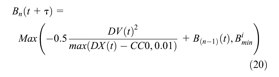
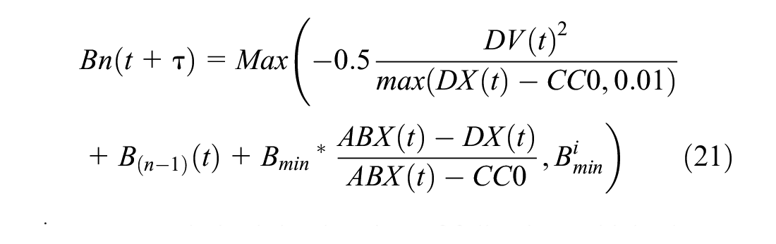
iv. Emergency braking regime
The existing acceleration equation according to ( 23 ) is:
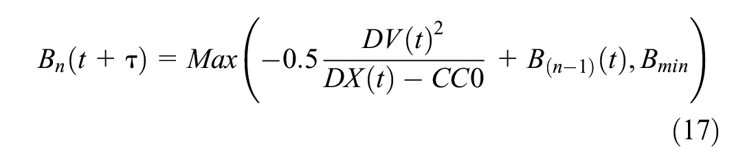

In the existing equation, when the relative speed is near 0, there are chances of Bn becoming positive as the leader can have any acceleration value. Also, it assumes that the driver will decelerate even if the leader is accelerating, that is, for a negative relative speed.
Modifications 2 and 3 from the closing regime are also applicable here. Two more modifications include:
For negative relative speed, there is no need for the follower vehicle to decelerate (so acceleration is set to zero).
An additional term (
If DV < 0

Otherwise,
If
Once the acceleration values are estimated for the regimes, the speed and position are calculated using numerical integration methods.
Numerical Integration Methods for Speed and Position Calculation
For the calculation of speed and position from acceleration, numerical integration equations are used. Several popular methods such as the Euler Cromer method, Midpoint method, Velocity Verlet method, and Beeman method have been reported in the literature to be suitable for computing speed and positions from Newton’s equation of motion ( 33 ). The most appropriate can be problem-specific and needs to be evaluated on the desired data set. Thus, these numerical integration methods are applied to predict leader speeds and positions based on observed acceleration profiles. The results are discussed below.
The equations for various methods are shown below ( 33 ):
Euler Cromer Method:


Midpoint method:

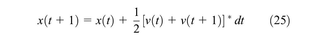
Velocity Verlet Method:
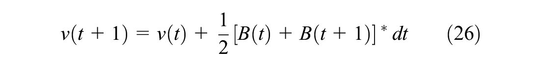
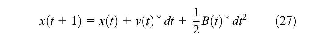
Beeman method:
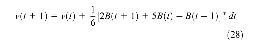
where
v(t + 1) = speed at next time step,
x(t + 1) = position at next time step,
B(t) = acceleration at current time step,
B(t + 1) = acceleration at next time step, and
B(t − 1) = acceleration at previous time step,
dt = time step.
The Goodness of Fit Function Used for Calibration
The goodness of fit function for calibration is the deviation between observed and computed speeds. Thus, calibration is formulated as an optimization problem to determine the best set of model parameter values, which minimizes this RMS error.
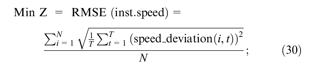

Thus
In this study, out of 10 W-99 parameters (CC0–CC9), seven are calibrated: CC1, CC2, CC3, CC4, CC5, CC7, and CC8. CC0 is determined by measuring the gaps in a drone image of the stopped vehicles at a signal. CC0 for two-wheelers is taken as 0.4 m, and 0.66 m for cars, the default value of CC6 is adopted in this study as in Raju et al. ( 6 ). Durrani et al. ( 7 ), and CC9 is not used in the modified equations.
Other fixed values used in calibration include the desired speed, maximum deceleration rates (cf. Table 2), and the reaction time (τ) which is taken as 1.0 s based on empirical analysis conducted by authors.
Kinematic Parameters of Mixed Traffic Flow
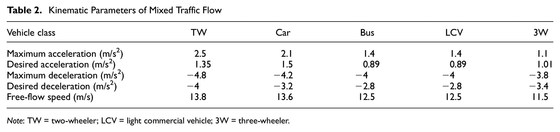
Note: TW = two-wheeler; LCV = light commercial vehicle; 3W = three-wheeler.
The optimization-based calibration process determines a set of CC parameters for a given class that yields the minimum RMSE. This procedure is done separately for the vehicle classes two-wheelers and cars. For the calibrated values of CC parameters, RMS errors for acceleration and position are also computed based on the deviation between the observed and predicted values.
Results and Discussion
Analysis Methodology
For calibration and validation purpose, leader–follower pairs are randomly divided into 70% (Pairs: TW = 250, Car = 200 with Datapoints: TW = 6,710, Car = 5,748) for the estimation and 30% holdout data for the validation. The model is calibrated using the estimation data set and validated by calculating performance measures with the calibrated model on the holdout data set.
This study is analyzed with the following methodology:
The W-99 model is calibrated by using existing acceleration equations and proposed acceleration equations to evaluate the effect of the equations’ modifications.
Alternative numerical integration schemes are evaluated to find the method which gives accurate predictions for acceleration, speed, and position over time.
The proposed W-99 calibrated model is compared with other calibrated W-99 models by evaluating the performance measures, RMSE of acceleration, instantaneous speed, and position.
Different driving behavior of two-wheelers and cars are evaluated from their CC values and gap-relative speed plots.
Leader–follower pairs are classified into strict and overlapping staggered following based on the lateral overlap; calibration analysis is done for these pairs.
Table 3 shows the calibrated CC parameters according to the existing acceleration equation and proposed acceleration equations; CC parameters by heuristic methods; the goodness of fit of these parameters; and, for validation, a data set for two-wheelers and cars.
Calibrated CC Parameters and Goodness of Fit Using Existing and Proposed Acceleration Equations and Heuristic Methods
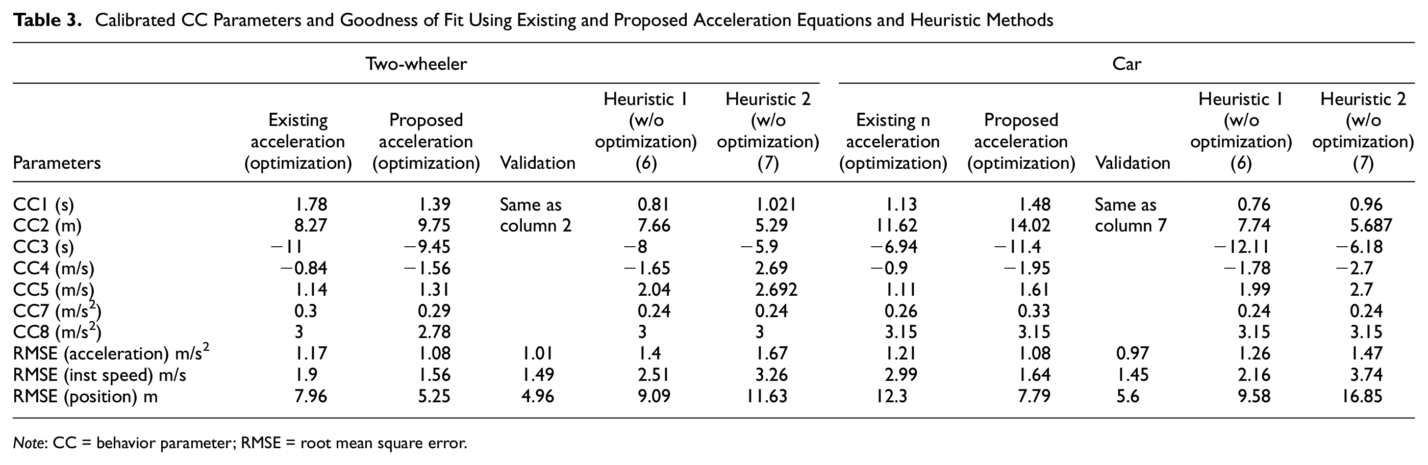
Note: CC = behavior parameter; RMSE = root mean square error.
The results of calibration by existing acceleration equations (columns 1 and 6) and by proposed acceleration equations (columns 2 and 7) are explained below.
The results of calibration by Heuristic 1 (columns 4 and 9) and Heuristic 2 (columns 5 and 10) are explained below.
Performance on the Holdout Set
For the holdout data (30%), the performance measures are computed using the CC parameters obtained after calibration using the proposed equations; the result is given in columns 3 and 8 in Table 3. From the results, the calibrated model parameters also perform well on the validation data set.
Use of Modified Acceleration Equations
Position, speed, and acceleration profiles predicted by existing acceleration equations and the proposed acceleration equation are plotted along with observed profiles for a sample follower in Figure 8.
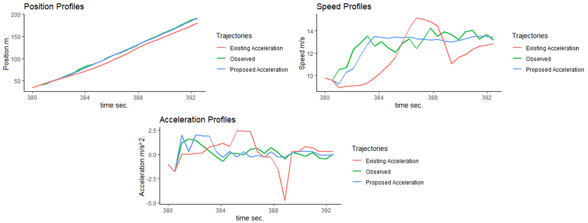
Trajectory profiles with modified and existing acceleration equations.
From Figure 8, the model with proposed acceleration equations predicts the observed trajectories better than the model with existing acceleration equations. This is also observed in Table 3, where the RMSE of the proposed acceleration equations are lower for speed (RMSE [m/s]: 1.56 versus 1.9), position (RMSE [m]: 5.25 versus 7.96), and acceleration (RMSE [m/s2]: 1.08 versus 1.17) than for the existing equations for two-wheelers. Similar trends are also observed for cars.
Evaluation of Numerical Integration Methods for Trajectory Computation
Numerical integration methods are evaluated based on deviation speeds and position profiles relative to the observed trajectories. Figure 9, a and b, shows the plot of absolute deviation of speed and absolute deviation of position by the different methods with observed speed and position of a sample leader respectively. The goodness of fit is measured by the RMSE of predictions.
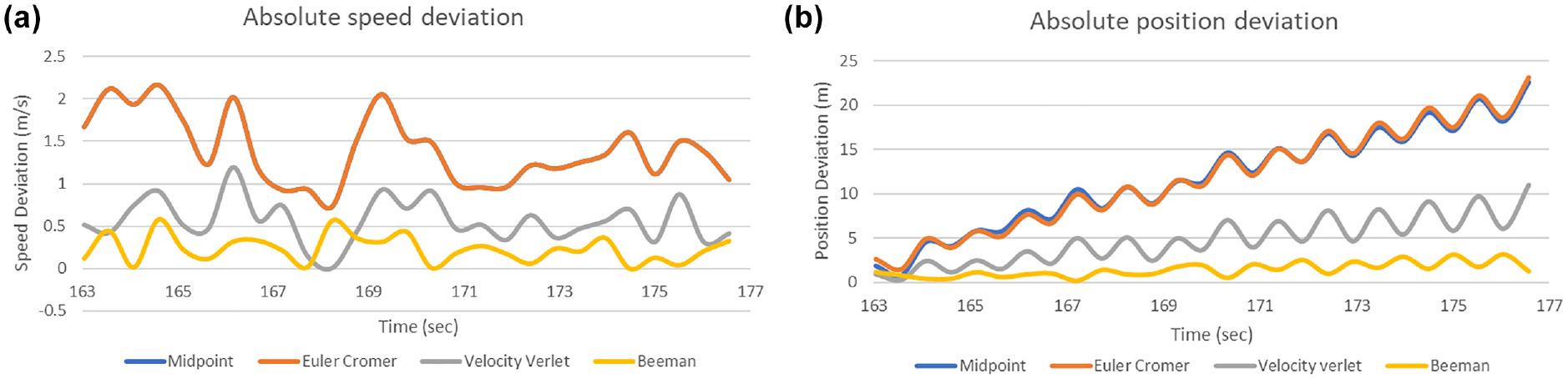
(a) Absolute speed deviation for different numerical integration methods; and (b) absolute position deviation for different numerical integration methods.
The average RMSE between observed values and calculated values of speed and position are computed for all different methods across all different leaders.
RMSE of speed for midpoint method: 1.438 m/s, Euler Cromer method: 1.438 m/s, Velocity Verlet method: 0.606 m/s, and for Beeman method: 0.282 m/s.
RMSE of position for midpoint method: 12.701 m, Euler Cromer method: 12.701 m, Velocity Verlet method: 5.345 m, and for Beeman method: 1.692 m.
The RMSE is smallest for Beeman’s method for both speed and position computations and this method is, therefore, used subsequently.
Comparison With Other W-99 Models
W-99 parameters are calibrated for the given data set using procedures provided by Raju et al. ( 6 ) and Durrani et al. ( 7 ), denoted as the heuristic method 1 and 2, respectively. The heuristic 1 method is chosen because they have used the same data as in this paper to calibrate the W-99 model; heuristic 2 is considered as they have considered heterogeneity across the vehicle types and pairs. As noted earlier, these heuristic methods calculate W-99 parameters without minimizing the deviation from observed field data.
For comparison, the proposed parameters and fit functions were compared with other calibration results in the literature for multi-lane mixed traffic conditions based on macroscopic performance measures.
Figure 10 shows the deviation of the sample predicted trajectory of the follower (two-wheeler) by different W-99 models with observed trajectory.
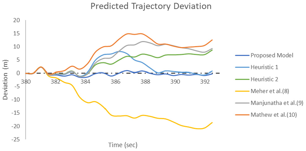
Predicted trajectory deviation.
The results of performance measures by the proposed model, heuristic models, and other calibration results in the literature are plotted in Figure 11.
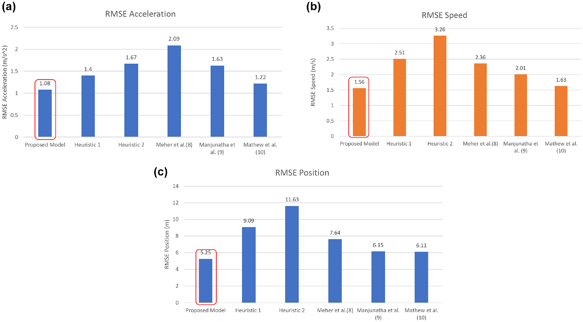
(a) RMSE acceleration for different W-99 models; (b) RMSE speed for different W-99 models; and (c) RMSE position for different W-99 models.
Following the plot in Figure 11, a to c, shows the RMSE of acceleration, speed, and position respectively for different calibrated W-99 Models for two-wheelers as a class of follower.
From the above RMSE results, it can be seen that the performance measures by the proposed method offer a significant improvement in predicting acceleration, speed, and position at the microscopic level.
Difference in Vehicle-Following Parameters and Thresholds Between Two-wheelers and Cars
Figure 12 shows the gap-relative speed plots with thresholds of regime identification, calculated for the CC parameters by the proposed method given in Table 3, for a constant leader speed of 10 m/s.
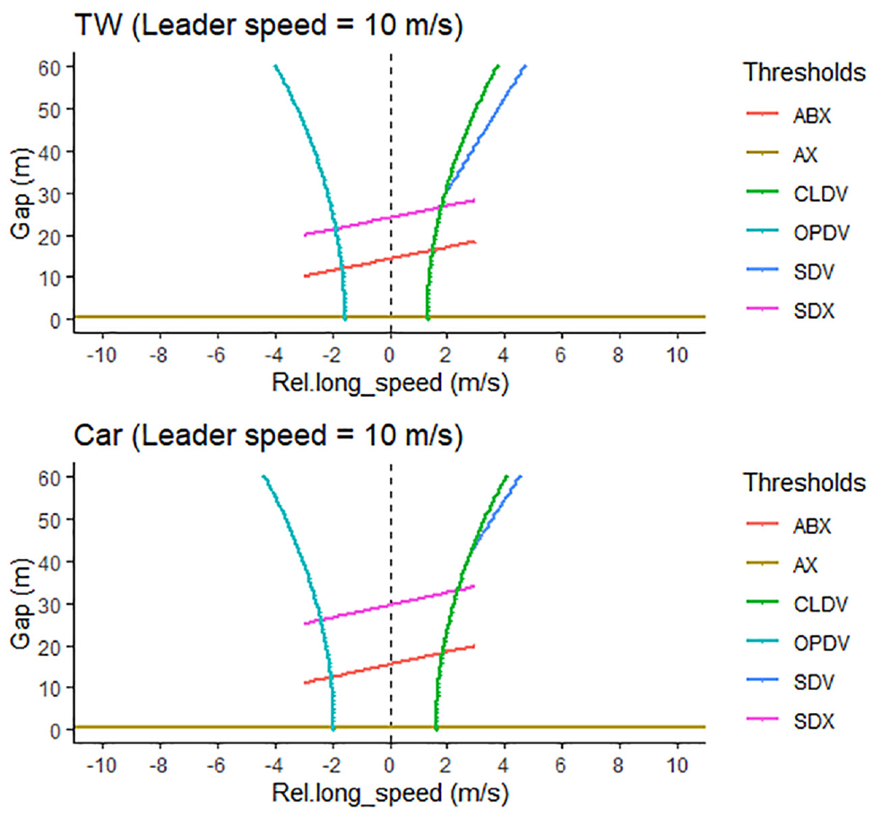
Wiedemann threshold plots for two-wheelers and cars.
From the calibrated W-99 parameters for two-wheelers and cars in Table 3 (columns 2 and 7) and threshold plots of the same parameters in Figure 12, we can see that the threshold diagram and the CC parameters are quantitatively different for these two vehicle classes.
CC1 of cars is larger than that for two-wheelers, which is evident as car drivers keep more of a gap to the leader than two-wheelers. The ABX for two-wheelers will, therefore, be lower than that for cars. Consequently, a lower percentage of two-wheeler points will be in the emergency braking regime than is the case for cars.
CC2 decides the range of the following regime; the value difference shows that cars have a longer following regime than two-wheelers, as SDX will be higher. Car drivers can, therefore, sense the change in leader behavior at a longer gap than two-wheeler drivers. Consequently, the chance of two-wheeler drivers being in the free-flow regime is higher compared with that of car drivers.
CC3 for two-wheelers is lower in magnitude than that for cars, which we can see as the slope of the SDV line in the threshold plot. Two-wheeler drivers, therefore, perceive a slow-moving leader and decelerate earlier than car drivers.
CC4 and CC5 gives the OPDV and CLDV thresholds; for two-wheelers, both CC4 and CC5 are smaller in magnitude than for cars. Two-wheelers are, therefore, more sensitive to a change in the leader’s speed.
CC7 is acceleration in the following regime: car drivers apply higher acceleration values than two-wheelers while following the leader unconsciously.
The most important observation is that, under the same relative speed and gap stimulus, two-wheelers and cars may be in different regimes and display different acceleration responses. Thus, accurate calibration of each vehicle’s parameters is essential for developing micro-simulation models for mixed traffic.
Analysis of Following Behavior Between Strict and Overlapping Staggered Following
A follower is considered to belong to the strict following regime if its overlapping width is more than 0.25 m for two-wheelers and more than 0.75 m for cars (i.e., 50% of the average width) for at least half of the observed time interval or if the smaller of the pair has a full overlap. Otherwise, the follower is considered to be in the overlapping staggered following regime, these criteria are based on empirical analysis conducted by authors. 276 two-wheelers and 328 cars were in the strict following regime, whereas 268 two-wheelers and 152 cars were classified into the staggered following regime. The calibration analysis is done for strict and overlapping staggered. The calibrated parameters and the goodness of fit (RMSE [acceleration] m/s2, RMSE [speed] m/s, RMSE [position] m) for the above four sets of CC’s are given in Table 4.
Calibrated CC Parameters and Goodness of Fit for Strict and Overlapping Staggered Following
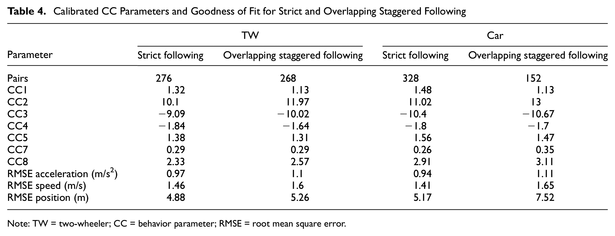
Note: TW = two-wheeler; CC = behavior parameter; RMSE = root mean square error.
Figure 13, a and b, shows the gap-relative speed plots with thresholds of regime identification for the CC parameters of strict and overlap-staggered following for two-wheelers and cars as given in Table 4, for a constant leader speed of 10 m/s.
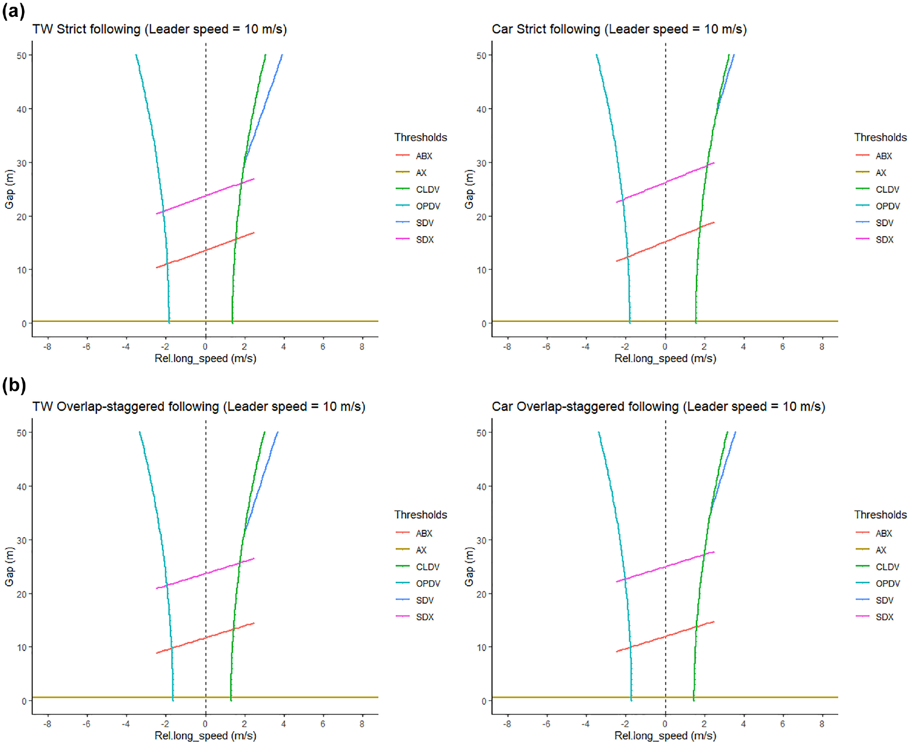
(a) Wiedemann threshold plots, strict following for TW and cars; and (b) Wiedemann threshold plots, overlapping staggered following for TW and cars.
The calibration results indicate that the driving behavior in a staggered car-following situation is different from that of strict car-following. This is particularly true for the safety indicator time to collision, that is, the ratio of gap (DX) and relative speed (DV) ( 34 ). Different parameter sets are, therefore, to be calibrated for strict and staggered following.
The CC1 values for strict and staggered following imply that drivers keep a smaller gap in staggered following compared with the strict following. The values found for CC4 and CC5 imply that, in the staggered following, drivers are more sensitive to changes in leader speed than the strict following. There are also differences with respect to the vehicle classes: two-wheeler drivers are found to keep lower gaps and to be more sensitive to speed changes of a leader than car drivers.
Conclusion
This paper proposes and implements a calibration procedure for the Wiedemann-99 model based on RMSE between simulated and observed trajectories of mixed traffic consisting predominantly of motorized two-wheelers and cars. The proposed modifications of the Wiedemann acceleration equations allowed for a more realistic representation of driving behavior under these conditions. Alternative numerical integration schemes for computing speed and position over time are evaluated. The performance of the proposed calibration method is compared with other heuristic trajectory-based calibration methods. The calibrated parameters may help understand the dynamics of mixed traffic flow. In particular, we found differences in the car-following behavior between motorized two-wheelers and cars as well as between strict and overlapping staggered following.
The following key findings and observations emerge from this study. The simulation-based analysis demonstrates that different microscopic W-99 parameters can lead to similar macroscopic performance measures. Thus, the psychophysical (Wiedemann model) calibration using macroscopic and aggregate performance measures may not uniquely determine microscopic behavior or performance.
Existing acceleration equations reported in the context of W-99 models can lead to some inconsistency and unrealistic driving behavior characteristics. These include the inability to capture vehicle type-specific features and a wrong sign for acceleration in some cases. Modifications are proposed to these equations to be consistent with observed driving behavior.
The microscopic performance of the above model in computing trajectories depends on the calibration parameters and is also quite sensitive to the numerical integration technique. Five different methods were evaluated, and it was observed that Beeman’s integration scheme provides the best fit with the observed data.
An optimization-based scheme is used to calibrate the W-99 model for mixed traffic with the above modifications. The proposed calibration scheme is found to outperform other calibration methods based on trajectory data (but without optimization) in RMSE for speed, position, and acceleration. The calibrated parameter values for thresholds and boundaries for regimes turned out to be behaviorally more realistic than those produced with other methods. Visual comparison of the regimes across models confirms these differences.
Not only do the parameters and the regime boundaries vary across calibration methods, but they also differ between two-wheelers and cars in mixed traffic. These differences are quantified and illustrated using sample plots of relative speed and gap across vehicle classes. The results reveal that the calibrated parameter values and, consequently, the thresholds that delineate closing, following, emergency braking, and opening regimes vary between two-wheelers and cars. The window (in the relative speed versus gap plot) for the unconscious following is larger for cars, while the free-flow regime is more extensive for two-wheelers. Under the same relative speed and gap stimulus, two-wheelers and cars may be in different regimes and display different acceleration responses.
The study’s findings have direct and vital applications for the calibration and development of mixed traffic micro-simulation models. This study is based on calibration from a midblock section in a divided six-lane arterial in Chennai. Extending this study to other locations and considering extended car-following behavior such as vehicle platooning would be a possible direction for continuing research. Extending the analysis to consider other facility types (four-lane divided urban roads, two-lane divided and undivided roads) as well as intersections by choosing suitable performance measures is an exciting and challenging direction for future work.
This work can be extended to other simulation platforms, including Sumo, Aimsun, Simtraffic, and so forth, since all models belong to the same class of car-following models (local time-continuous models or iterated maps with speed, relative speed, gap, and sometimes acceleration as exogenous variables). More systematic studies that relax the conditions to identify leader–follower pairs (in duration of the following or extent of lateral overlap), allowing analysis of more diverse leader–follower pairs, are being investigated by the authors and will be reported in future studies. Furthermore, the analysis can be extended to model not just the leader but the whole local traffic environment as explicit input allowing for many other maneuvers beyond the scope of this particular study.
Footnotes
Acknowledgements
The authors express sincere thanks to four anonymous reviewers for their constructive suggestions.
Author Contributions
The authors confirm contribution to the paper as follows: study conception and design: A. A. Chaudhari, K. K. Srinivasan, B. R. Chilukuri, M. Treiber, O. Okhrin; data collection: not applicable; analysis and interpretation of results: A. A. Chaudhari, K. K. Srinivasan, B. R. Chilukuri, M. Treiber, O. Okhrin; draft manuscript preparation: A. A. Chaudhari, K. K. Srinivasan, B. R. Chilukuri, M. Treiber, O. Okhrin; All authors reviewed the results and approved the final version of the manuscript.
Declaration of Conflicting Interests
The author(s) declared no potential conflicts of interest with respect to the research, authorship, and/or publication of this article.
Funding
The author(s) disclosed receipt of the following financial support for the research, authorship, and/or publication of this article: This work is supported by scholarships through MHRD Government of India, Partial Support from pCOE from IIT Madras through project no. SB20210831CEMHRD008432 and DAAD (The German Academic Exchange Service) fellowship at TU Dresden.