Detecting and Rectifying Vehicle Malicious Misbehavior for Intersection Movement Assist: A Sensor-Based Misbehavior Detection Study

Abstract

Recent developments in wireless communication technologies have led to the evolution of connectivity between vehicles. Maintaining connectivity between vehicles increases a vehicle’s awareness of other nearby vehicles, which can be used in safety applications. Identification of malicious misbehaving vehicles plays an important role in road safety. This research establishes the minimum detectable error (MDE) boundary for relative position between the observer and status vehicles (SV) using vehicle sensor and GPS error profile from field tests and established minimum standards. The results demonstrated that the MDE increases in the lateral direction (side-to-side) with the increase in relative distance between the observer and status vehicles (OV and SV) while remaining the same in the longitudinal direction (front-to-back). This research effort explores the use of Sensor-Based Misbehavior Detection (SBMD) with current specifications and the defined MDE boundary for implementation in the Intersection Movement Assist (IMA) safety application to rectify false positive and false negative hazard messages propagated by a malicious misbehaving vehicle. The simulation approach used in this research quantifies the total number of false positive/negative hazard detections received by a third-party vehicle (TPV) using the IMA safety application and assesses the capability of the OV equipped with SBMD to rectify the false positive/negative hazard detection. In cases where there was no hazard, SBMD produced an 83% to 90% improvement in the reduction of false positive hazard detections. In the cases with hazard scenario, where the SV is in the not-safe-to-cross zone, SBMD produced an 80% to 99% improvement in application performance.

Keywords

operations traffic simulation automated/autonomous/connected vehicles vehicle-highway automation sustainability and resilience transportation systems resilience transportation infrastructure protection and preparedness AMR10 cyber security

The Sensor-Based Misbehavior Detection (SBMD) Analysis and Simulation project is intended to assess the effectiveness and feasibility of using onboard vehicle sensors and sensor systems to detect and mitigate connected and automated vehicle misbehavior in the field caused by the transmission of erroneous basic safety message (BSM) data. One of the key outcomes from this approach is that any observed misbehavior can be reported together with an accurate assessment of the difference between the BSM data and ground truth.

With the growing number of electronic features in cars and their connections to the cloud, smartphones, road-side equipment, and neighboring cars, the need for effective cybersecurity is paramount ( 1 ). Vehicles that include interactive advanced driver-assistance systems (ADAS) and cooperative intelligent transport systems (C-ITS) can be regarded as connected ( 2 ). Connected-vehicle safety applications are designed to increase situational awareness and mitigate traffic accidents through vehicle-to-vehicle (V2V) and vehicle-to-infrastructure (V2I) communications ( 2 ). ADAS technology can be based on vision/camera systems, sensor technology, vehicle data networks, V2V, or V2I systems ( 2 ). Increased automation exacerbates any risk by increasing the opportunities for an adversary to implement a successful cyber-attack ( 3 ). Several GPS spoofing detection techniques and patents have been developed to mitigate malicious behavior but are generally ineffective against attacks on body or vehicle mounted GPS receivers where the environment is dynamic ( 4 ). Besides intentional malicious behavior in reporting the false location and trajectory of vehicles, local environmental factors may degrade the accuracy of reported vehicles’ locations. Global navigation satellite systems (GNSS) suffer from signal blockage and severe multipath in urban canyons, which degrade their positioning accuracy and availability ( 5 ).

Automated vehicle systems rely heavily on onboard sensors such as cameras, radar/lidar, and GPS as well as on capabilities such as 3G/4G connectivity and V2V/V2I communication to make real-time maneuvering decisions ( 6 ). The vehicle control imposes very strict requirements on the security of the communication channels used by the vehicle to exchange information as well as the control logic that performs complex driving tasks such as adapting vehicle velocity or changing lanes ( 6 ). Previous studies, including one by Guo and Coifman, have focused on the detection of GPS positioning errors from a probe vehicle equipped with lidar and Differential Global Positioning System (DGPS) ( 7 ). A correlation approach is used to detect GPS positioning errors and prevent incorrect classifications of the targets caused by erroneous projections between the vehicle coordinate system and the world coordinate system ( 7 ). To take full advantage of connected-vehicle technology in most safety applications, precise vehicle positioning information is needed in addition to V2V communication ( 8 ). A field study by Peng et al. using standard GPS receivers and dedicated short-range communication (DSRC)-based V2V communication was conducted to acquire the relative trajectories of vehicles traveling in multiple lanes toward a merging junction with an accuracy of less than half of the lane width ( 8 ). A proposed scheme by Lim et al. ( 9 ) uses unique ADAS sensor data such as digital fingerprints, without the involvement of infrastructure and third-party trusted authority in a vehicular ad hoc network (VANET). Other patents were developed to allow for the use of a less accurate version of the GPS-receiver necessary for automated steering of an automated vehicle through GPS data correction ( 10 ).

Connected-vehicle safety applications are designed to increase situational awareness and to mitigate traffic accidents through V2V and V2I communications ( 2 ). Features may include adaptive cruise control, automatic braking, GPS and traffic warnings, connections to smartphones, alerts the driver to hazards, and keeping the driver aware of what is in their blind spot ( 2 ). Among these applications likely to have a substantial impact on daily travel patterns is the Intersection Movement Assist (IMA) safety application. IMA has been recognized as one of the countermeasures most prominent in reducing angle crashes at intersections, which constitute 22% of all crashes in the United States ( 11 ). Using vehicle-based sensors, V2V, and V2I communications, IMA offers extended vision to provide early warning of an imminent crash ( 11 ).

This research focuses on the effectiveness of the SBMD concept in observing and identifying misbehavior by the status vehicle (SV). This focus includes the scale of vehicle status message (VSM) errors that can reliably be detected by an observer vehicle (OV) using conventional ADAS sensors. This is important because the OV sensors will only measure the relative position and dynamic parameters (speed, heading, etc.) relative to the OV. This means that the OV must use its own position, speed, and heading data to convert the sensor data to the world reference frame (which is how the VSM data is provided) so that the VSM data can be compared with the sensor data. The result is that errors in the OV state will be compounded on the sensor measurements, thereby limiting the scale of detectable VSM data errors. The implementation of the IMA safety application is used in this research effort to quantify the number of false positive/negative hazard messages. The results are then compared against the implementation of SBMD to assess the system’s ability to rectify the number of false positive/negative hazard messages caused by malicious misbehavior. In the context of this study, malicious misbehavior by the SV is defined as the intentional misrepresentation of the SV’s true location (e.g., GPS spoofing) causing either a false positive or negative hazard detection.

The objective of this research is to assess the effectiveness of SBMD capability in detecting malicious misbehavior by SVs under varying relative positions between the SVs and IMA hazard thresholds. The SV’s true and malicious locations were varied under several scenarios to simulate varying degrees of intentional reported location deviation from the SV’s true location. The results from this research effort will inform the scenarios in which, under IMA implementation, SBMD can effectively detect and rectify an instance of malicious misbehavior by the SV.

Methodology

This section describes the methodology used for the field data collection, the references for the vehicle sensor error profile, establishing the minimum detectable error (MDE), set-up of the Monte Carlo simulation, and simulation scenario design.

Field testing was designed and conducted to collect the field reading of conventional advanced driver-assistance system sensors against their ground truth to develop error profile models. These error profiles were later used in a Monte Carlo simulation to establish an MDE boundary and then used subsequently in quantifying the probability for detecting vehicle malicious and erroneous misbehavior. Finally, this paper leverages a simulation approach to assess the impacts of SBMD on IMA safety application in rectifying false positive/negative hazard messages caused by malicious misbehavior.

Field Data Collection for Vehicle Sensor Error Profile

This section discusses the references and field tests used to develop the error profile model used in the Monte Carlo simulation. The vehicle sensor error profile was developed from field testing with the procedures described in this section. The vehicle GPS error used for this study follows the standards highlighted in SAE Standard J2945 ( 12 ). The vehicle heading error profile used follows the recommendations outlined in a separate study under FHWA report FHWA-JPO-17-483 ( 13 ). This value for heading error was used instead of the requirement specified in SAE J2945 because this is consistent with most heading sensors available today. The requirement provided in SAE J2945 was not originally intended to be used for the purposes identified in SBMD. As a result, rather than using the specification, a realistic value available from commercial sensors was used instead.

A vehicle sensor field test was conducted to quantify the vehicle lidar and radar error profiles for both range and angle detection. The vehicle sensor error profiles for range and angle were incorporated into the MDE Monte Carlo simulation. Figure 1 shows an example of an OV reported versus a true relative angle and distance to the SV. The error is a result of vehicle sensor error imposed on the true measurement value.

Figure 1.

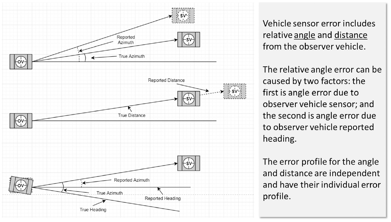
Example of relative angle and distance error generator.

The relative position measured between the observer and SVs in distance and angle will affect the error profile deviations. The measured relative position of the SV from the OV is reported as:

D for Distance

θ for Angle.

Figure 2 shows the graphical illustration of the relative distance and angle of the SV from the OV.

Figure 2.

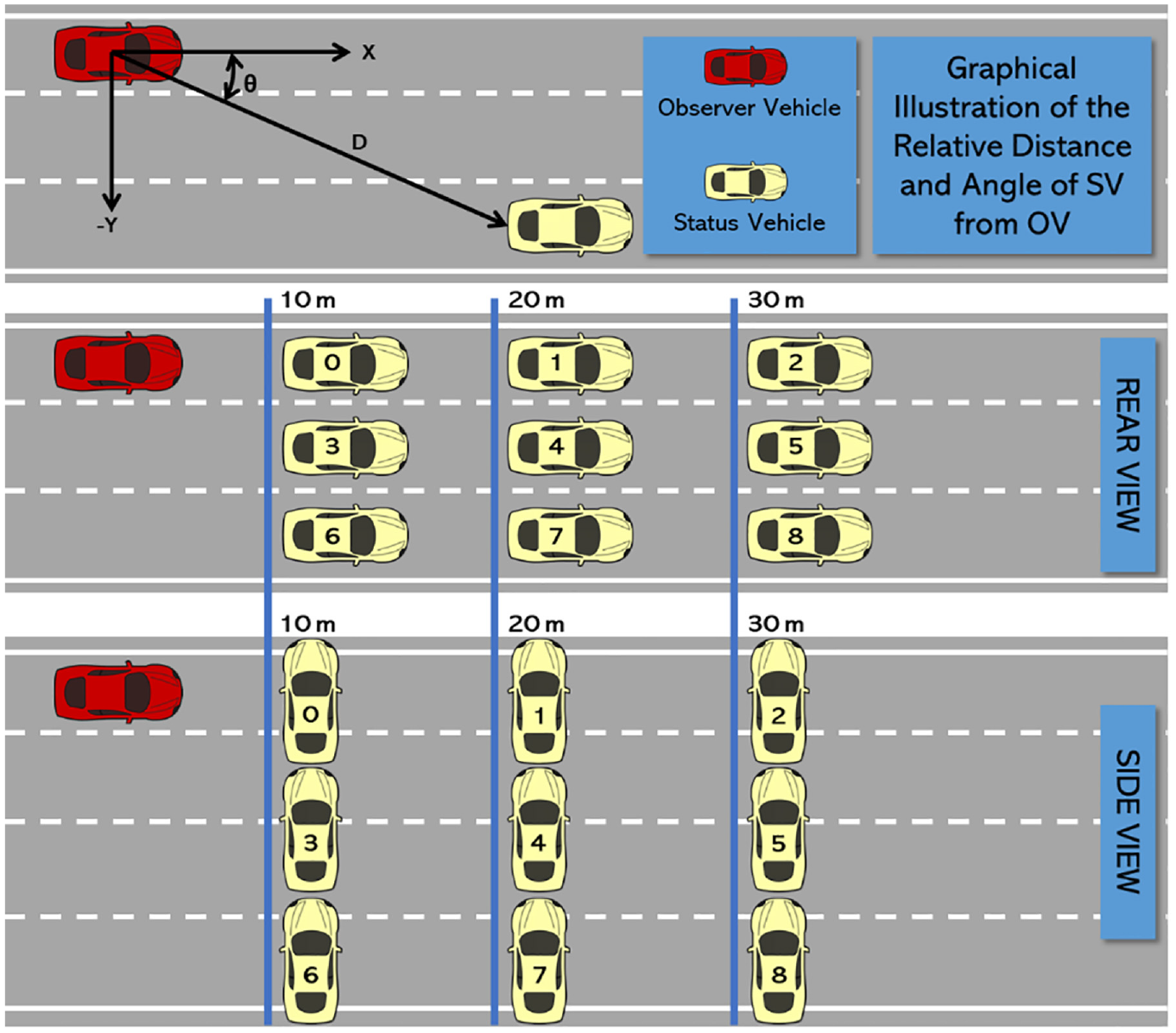
Illustration of status vehicle test locations relative to the observer vehicle.

A series of a minimum of 1,000 observations where both lidar and radar were taken for each of the test locations is shown in Figure 2. Figure 3 shows examples of the rear and side views of the SV during the lidar and radar field test. The field study was conducted in clear and dry weather. The lidar used for the field testing was a Velodyne Ultra Puck while the radar used was a Delphi ESR 2.5.

Figure 3.

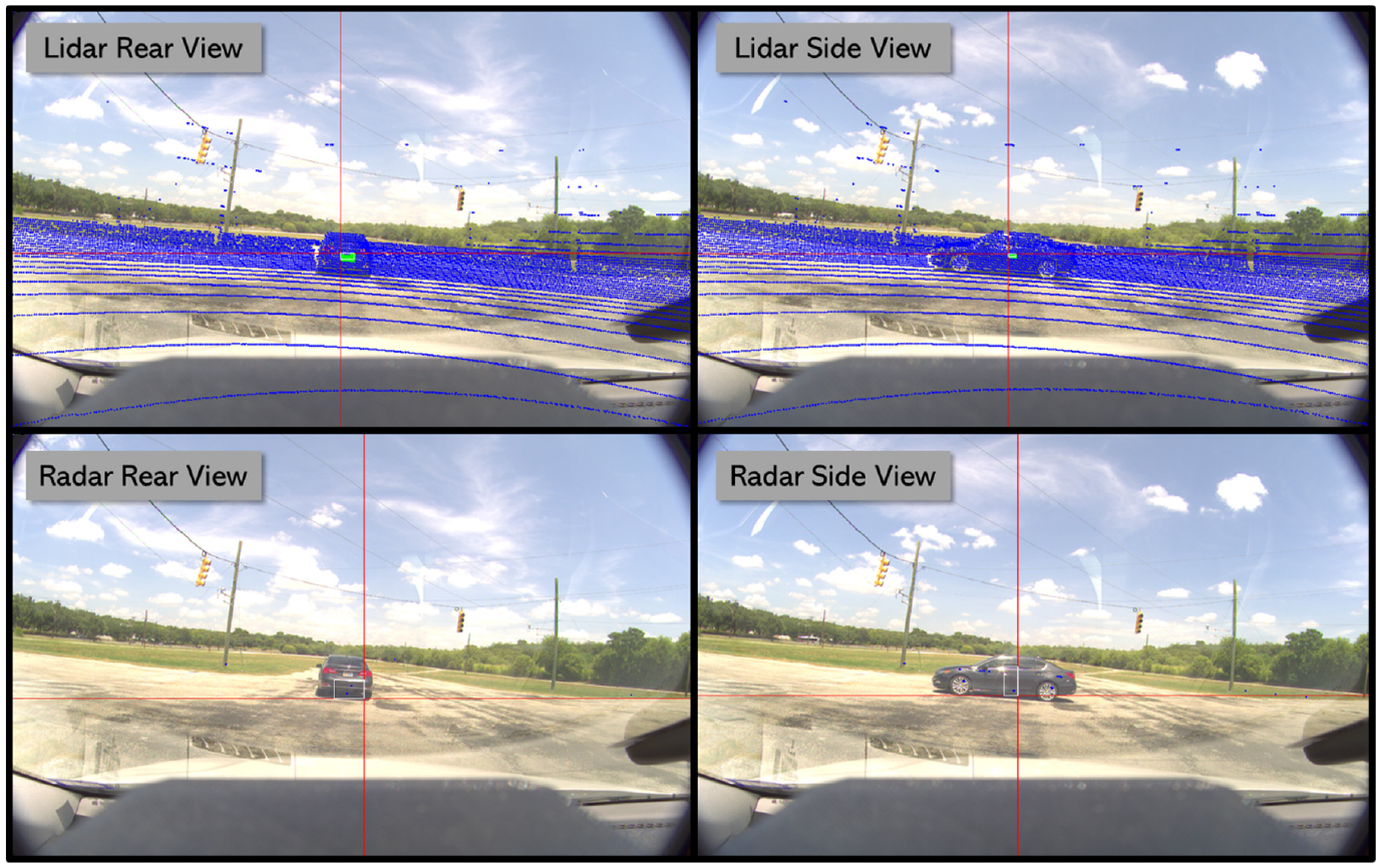
Wide angle view of lidar and radar field testing for status vehicle rear and side.

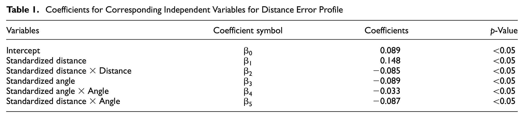
Using the data collected from the field test, a multivariable linear regression was coded in R scripting language to develop the following one standard deviation from the mean distance predictive model. A sensitivity analysis was performed considering the possible combinations of the variables presented in equations 1 and 2. Of the field data, 10% was used as a test set to evaluate the performance of both models based on the R² value. Based on the analysis results, the models presented in equations 1 and 2 yield the highest R² value.

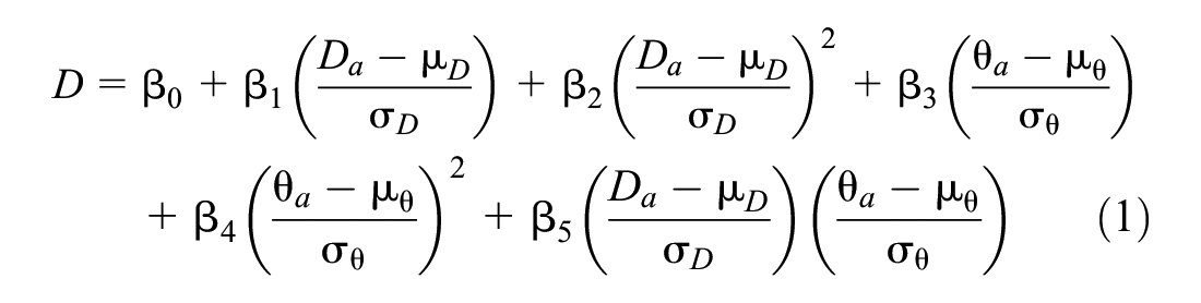
D = β_{0} + β_{1} (\frac{D_{a} - μ_{D}}{σ_{D}}) + β_{2} {(\frac{D_{a} - μ_{D}}{σ_{D}})}^{2} + β_{3} (\frac{θ_{a} - μ_{θ}}{σ_{θ}}) + β_{4} {(\frac{θ_{a} - μ_{θ}}{σ_{θ}})}^{2} + β_{5} (\frac{D_{a} - μ_{D}}{σ_{D}}) (\frac{θ_{a} - μ_{θ}}{σ_{θ}})

(1)

where

D = one standard deviation of the mean (m),

β_n = corresponding coefficient to the independent variable,

D_a = actual relative distance from the OV (m),

μ_D = mean for measured distance (m),

σ_D = standard deviation for measured distance (m),

D_θ = actual relative angle from the OV (degrees),

μ_θ = mean for measured angle (degrees),

σ_θ = standard deviation for measured angle (degrees).

Table 1 shows the list of corresponding coefficients to each independent variable in predicting the expected standard deviation for measured distance by varying the true distance and angle.

Table 1.

Coefficients for Corresponding Independent Variables for Distance Error Profile

Variables	Coefficient symbol	Coefficients	p-Value
Intercept	$β_{0}$	0.089	<0.05
Standardized distance	$β_{1}$	0.148	<0.05
Standardized distance × Distance	$β_{2}$	−0.085	<0.05
Standardized angle	$β_{3}$	−0.089	<0.05
Standardized angle × Angle	$β_{4}$	−0.033	<0.05
Standardized distance × Angle	$β_{5}$	−0.087	<0.05

Similar to the distance error profile, a multivariable linear regression was coded in R scripting language to develop the following one standard deviation from the mean angle predictive model.

θ = γ_{0} + γ_{1} (\frac{D_{a} - μ_{D}}{σ_{D}}) + γ_{2} {(\frac{D_{a} - μ_{D}}{σ_{D}})}^{2} + γ_{3} (\frac{θ_{a} - μ_{θ}}{σ_{θ}}) + γ_{4} {(\frac{θ_{a} - μ_{θ}}{σ_{θ}})}^{2} + γ_{5} (\frac{D_{a} - μ_{D}}{σ_{D}}) (\frac{θ_{a} - μ_{θ}}{σ_{θ}})

(2)

where

θ = one standard deviation of the mean (degrees),

β_n = corresponding coefficient to the independent variable,

D_a = actual relative distance from the OV (m),

μ_D = mean for measured distance (m),

σ_D = standard deviation for measured distance (m),

D_θ = actual relative angle from the OV (degrees),

μ_θ = mean for measured angle (degrees),

σ_θ = standard deviation for measured angle (degrees).

Table 2 shows the list of corresponding coefficients to each independent variable in predicting the expected standard deviation for measured distance by varying the true distance and angle.

Table 2.

Coefficients for Corresponding Independent Variables for Angle Error Profile

Variables	Coefficient symbol	Coefficients	p-Value
Intercept	$γ_{0}$	−0.055	<0.05
Standardized distance	$γ_{1}$	−0.027	<0.05
Standardized distance × Distance	$γ_{2}$	0.024	<0.05
Standardized angle	$γ_{3}$	0.390	<0.05
Standardized angle × Angle	$γ_{4}$	0.458	<0.05
Standardized distance × Angle	$γ_{5}$	0.038	<0.05

The error profiles included in the Monte Carlo simulations can be grouped into three primary sources: GPS-based error, heading-based error, and OV perception sensor-based error (e.g., lidar, radar, or camera). Below, we list the sources for each error profile used in the Monte Carlo simulation.

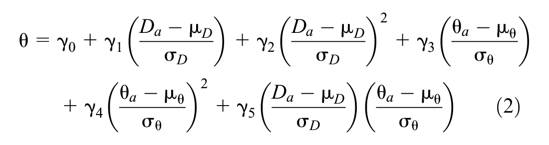
The GPS error profile used as part of the Monte Carlo simulation following the profile outlined under SAE Standard J2945:

The System shall set the DE_Latitude and DE_Longitude data elements to its corresponding 2-D horizontal position reference in the WGS-84 coordinate system.

The position of the system transmitting a BSM shall be accurate to within PosAccuracy of the vehicle’s actual 2-D horizontal position reference over 68% of the test measurements under open sky test conditions.

Figure 4 shows an example of the OV and SV reported locations versus their true location measured in latitude and longitude. The margin of error highlighted in the green ellipse illustration follows the error profile described in SAE Standard J2945.

Figure 4.

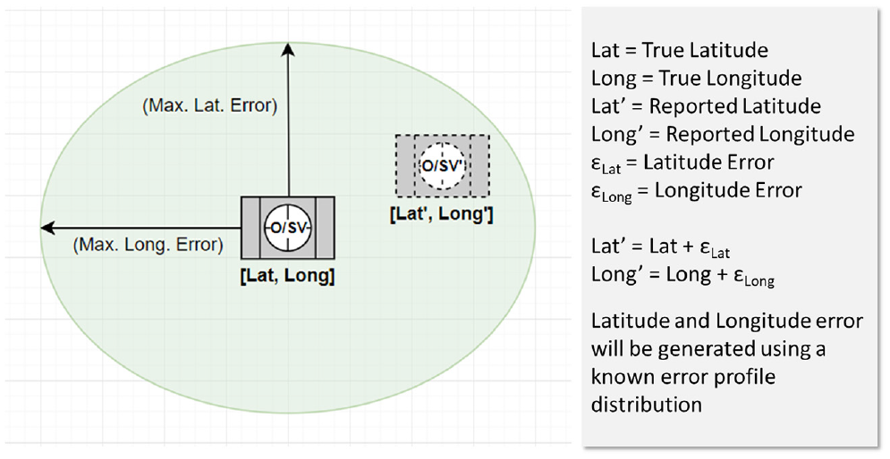
Illustration of latitude and longitude error generator.

The vehicle heading error tolerance used as part of the error profile for the Monte Carlo simulation follows the recommended threshold of 0.1 degrees as indicated in the FHWA report FHWA-JPO-17-483.

Defining the Minimum Detectable Error

As part of the misbehavior detection for OV to determine if an SV is outside its acceptable margin of error for reported location, the minimum detectable error (MDE) boundary is leveraged. The following describes the boundary construction of the MDE and the known error profile it considers:

Confidence interval: The MDE boundary first selects a confidence interval (e.g., 95th, 85th, 50th percentile) that will be used to identify the bounds of the known error profile.

Observer vehicle sensor error: The vehicle sensor error profile comprising range and angle using the distribution discussed in the previous sections from field test and previous study. This is the error from how the OV perceives the location of the SV.

Status vehicle GPS error: Using the error distribution described in SAE Standard J2945. This is the allowable error in the SV’s perception of its own location.

Observer vehicle GPS error: Using the error distribution described in SAE Standard J2945. This is the allowable internal OV GPS error experienced.

Observer vehicle heading error: Using the error distribution recommended from a separate study under FHWA report FHWA-JPO-17-483.

The OV must account for the allowable errors in the targeting sensors as well as allowable errors in both the SV and its own position based on GPS resolution. The three boundaries defined above using a constant confidence interval were summed together to define the MDE ellipse boundary. The OV needs to account for its own internal sensor and GPS error while accounting for the SV’s GPS error to define an MDE boundary.

If the SV reports itself to be outside this defined MDE boundary, the SV will be flagged as a misbehaving vehicle with the corresponding selected confidence interval. Figure 5 shows a graphical illustration of the SBMD classification of reported misbehavior.

Figure 5.

Summary of sensor-based misbehavior detection (SBMD) classification of reported misbehavior.

Misbehavior Classification

The reported results from each simulation run can be categorized into two groups as follows:

Misbehavior reported:

when the SV location reported in a VSM (e.g., BSM) is outside the MDE region;

misbehavior is detected and reported at the confidence used to determine the MDE.

No misbehavior reported:

when the SV location reported in a VSM (e.g., BSM) is within the MDE;

misbehavior cannot be confidently detected and therefore is not reported.

Monte Carlo Simulation of Minimum Detectable Error

Using the GPS and internal vehicle sensor error profiles described above, a series of Monte Carlo simulation scenarios was developed and simulated to construct the MDE boundary for the 95th confidence interval. The simulation includes cases where the SV is located between 10 and 70 m ahead of the OV in increments of 20 m then repeated for one and two lanes across. Figure 6 shows an illustration of the SV’s relative location from the OV when simulating the error profiles to develop the MDE boundary.

Figure 6.

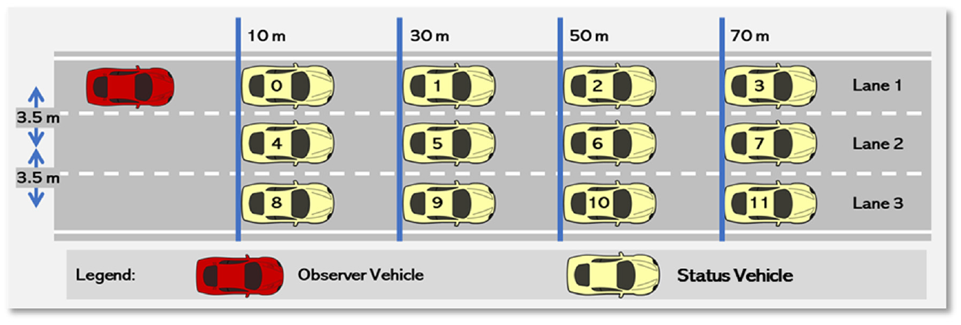
Illustration of the Monte Carlo simulation scenario to construct the minimum detectable error (MDE) boundary.

Each unique location was simulated using 100,000 random agents to achieve a statistically significant sample to define the MDE boundary. Table 3 lists the resulting lateral radius of the MDE by varying lane position and relative distance between the OV and SV. The results indicate a constant longitudinal radius of 3.5 m at all distances and lane positions between the OV and SV.

Table 3.

MDE Lateral Radius by Varying Lane and Relative Distance

Lane position	Relative forward position of SV from OV
Lane position	10 M	30 M	50 M	70 M
Lane 1 (same lane)	3.5 m	3.6 m	3.9 m	4.2 m
Lane 2 (one lane across)	3.5 m	3.6 m	3.9 m	4.3 m
Lane 3 (two lanes across)	3.5 m	3.7 m	3.9 m	4.3 m

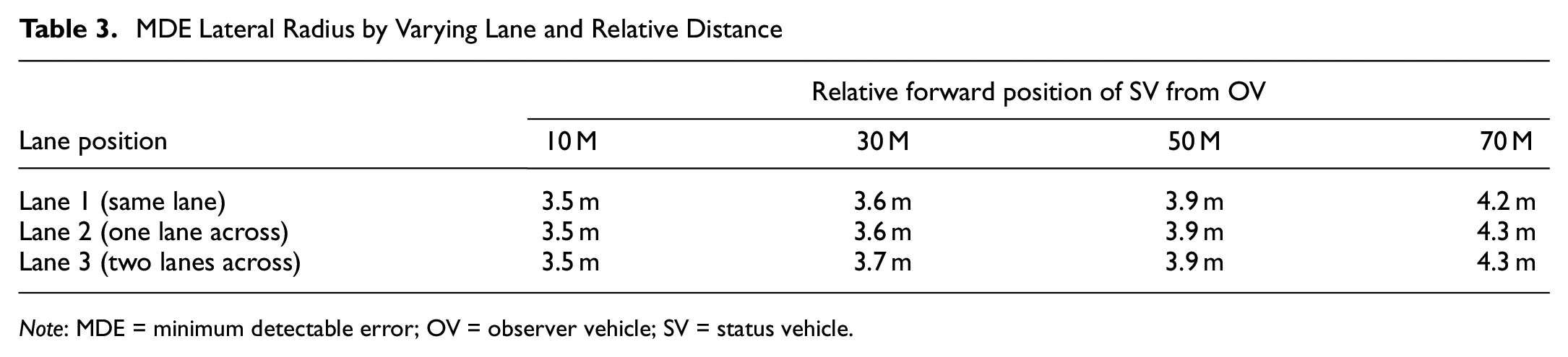
Note: MDE = minimum detectable error; OV = observer vehicle; SV = status vehicle.

The lateral radius of the MDE is seen to increase, while the longitudinal radius stays relatively constant, with the increase in relative distance between the observer and the SV. The change to vehicle location in adjacent lanes has insignificant impact on the MDE radius. Figure 7 shows an illustration of the increase in the MDE boundary in the lateral direction with the increase in distance between the observer and SV while the longitudinal radius remains constant.

Figure 7.

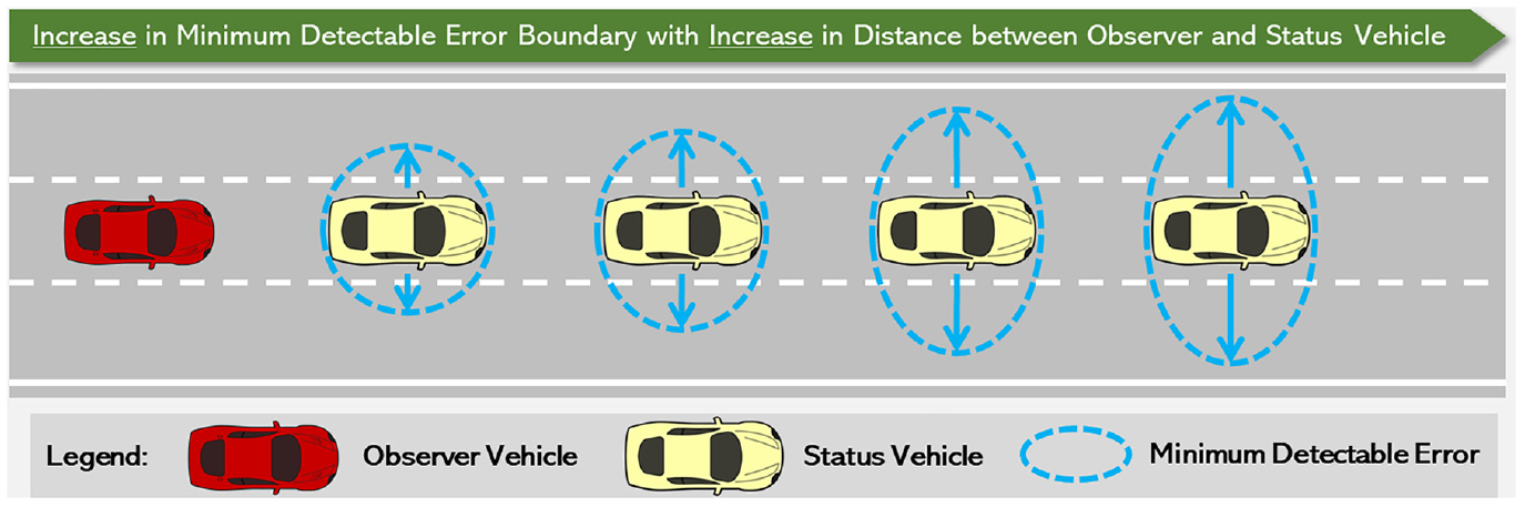
Illustration of increase in minimum detectable error (MDE) boundary in the lateral direction with increase in distance between observer and status vehicle (SV).

Intersection Movement Assist Simulation Approach and Analysis

The IMA application warns the driver of a vehicle when it is not safe to enter an intersection because of high collision probability with other vehicles at a stop sign or at controlled or uncontrolled intersections, for example, if another vehicle is running a red light or making a sudden turn. This application can provide collision warning information to the vehicle’s operational systems, which may perform actions to reduce the likelihood of a crash at the intersection. The IMA application provides several intersection crash avoidance (ICA) procedures such as Right Turn into Path, Left Turn into Path, and Left Turn Across Path/Lateral Direction. For the purposes of this research, the Straight Crossing Path was selected for simulation.

This section describes the modeling techniques used to simulate the IMA logic for gap acceptance, the construction of the simulation scenarios with and without SBMD implementation, and a discussion of the simulation results.

Safety Application Simulation Baseline Set-up

The safety applications assess other vehicles’ positions and trajectories to determine if the specific maneuver is deemed safe or not safe to execute. Within each safety application, TPVs receive BSMs from nearby vehicles in relation to their most recent trajectory and position. The TPV’s safety applications use the data within the BSM to determine if the vehicle sending the BSM (the SV) presents a hazard and notifies the driver if a maneuver is not safe to execute. Each BSM has inherent errors, such as GPS and heading error. Within the simulation, the message with GPS and heading error is compared with the message that would have been sent if calculated using the vehicles’ positions and trajectories without GPS and heading error (i.e., message with errors versus ground truth). This phase of the simulation provides a baseline for the safety application performance given inherent errors without implementing SBMD.

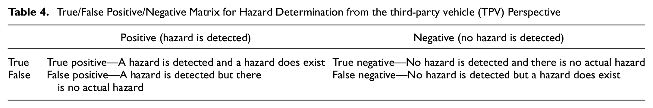
Table 4 shows a matrix for message classification and hazard determination from the perspective of a TPV in the four possible decisions made by the TPV when analyzing BSM data in connected-vehicle applications to identify hazards from messages with and without GPS and heading error.

Table 4.

True/False Positive/Negative Matrix for Hazard Determination from the third-party vehicle (TPV) Perspective

	Positive (hazard is detected)	Negative (no hazard is detected)
True	True positive—A hazard is detected and a hazard does exist	True negative—No hazard is detected and there is no actual hazard
False	False positive—A hazard is detected but there is no actual hazard	False negative—No hazard is detected but a hazard does exist

Once this baseline was established, a similar simulation was performed using assumed data from an OV. Essentially it was assumed that an OV had also received the same BSM the TPV was using to determine the presence of a hazard. The OV would then issue an Error Notification Message (ENM), and the TPV would redo its hazard determination based on this new information.

As with the baseline case, the simulations generate a set of TPV decisions, which contain some amount of error as a result of OV and SV errors. A key question then is to compare the frequency of these correct and erroneous decisions to assess the overall impact of SBMD on these applications.

Figure 8 shows the simulation and analysis framework for the safety application when comparing the hazard determination results from the perspective of the TPV with and without the SBMD capability.

Figure 8.

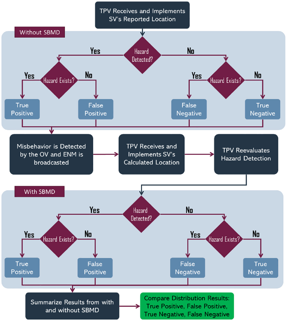
Simulation and analysis framework for evaluating the performance impact of SBMD on safety applications.

Intersection Movement Assist Gap Acceptance

The IMA gap acceptance determines if it is safe for the third-party vehicle (TPV) to execute an intersection crossing maneuver by calculating the most recent TPV and SV position and trajectories. The scenario assesses the case where the TPV is accelerating from a stopped position and attempting to make a thru movement at a two-way-stop control intersection. The crossing maneuver by the TPV is on a crossing path with the SV on the major road which has the right-of-way. If the SV with the conflicting path is below the IMA gap acceptance for the TPV to cross and clear the intersection, a “Do Not Enter Intersection” warning is presented to the driver of the TPV. The following describes the segments composed of the IMA gap acceptance for IMA side street thru movement. The following describes the segments composed of the IMA gap acceptance boundary.

Maneuver Time 1 (T1) = Time for TPV to accelerate to desired crossing speed (Acceleration)

Maneuver Time 2 (T2) = Time for TPV to complete crossing and clearing the intersection (Constant)

Maneuver Time 3 (T3) = Time for SV to reach the TPV’s conflicting path at constant speed (Time-to-Collision, Constant)

Figure 9 below shows the IMA gap acceptance zone segments listed above with each maneuver by the TPV and SV.

Figure 9.

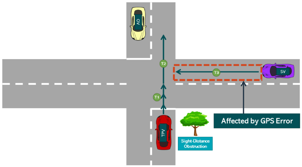
Intersection movement assist (IMA) time-to-collision segments.

Figure 9 highlights the segments that are calculated as a function of vehicle known locations that are affected by GPS error. The boundary of the IMA gap acceptance segments because of GPS error will result in the deviation of the threshold from its true value without GPS error, thus resulting in possible misclassification and incorrect hazard determinations.

Referring to the illustration shown in Figure 9, a TPV is at a complete stopped position behind the stop bar on the side street receiving recommendation whether if it is safe to enter, cross, and clear the intersection. The IMA safety application calculates and establishes the time-to-collision based on the current SV position and trajectory with respect to the time required by the TPV to enter, cross, and clear the intersection. If the SV’s time-to-collision is lower than the time required for the TPV to complete the crossing maneuver, a Do Not Cross warning is triggered within the TPV. If the SV time-to-collision is higher than the time required by the TPV to complete the maneuver, no warning is triggered within the TPV.

The later portion of the IMA safety application simulation analysis includes an OV within the sensor range to detect the SV and assess its reported location. If the SV’s BSM falls outside of the MDE, the OV reports it as a misbehavior and broadcasts an ENM. The TPV receives the ENM and redetermines whether the SV is within or outside the initially established Do Not Cross zone.

There are several factors that will cause a false positive or negative hazard determination by the TPV. The following are the factors considered for the IMA safety application:

GPS error from the SV that causes a false location of the SV within or outside of the IMA crossing zone boundary;

GPS error from the TPV that causes an error in the IMA crossing zone boundary.

Figure 10 shows an illustration of the two GPS errors above that are the primary cause of false positive or negative warning.

Figure 10.

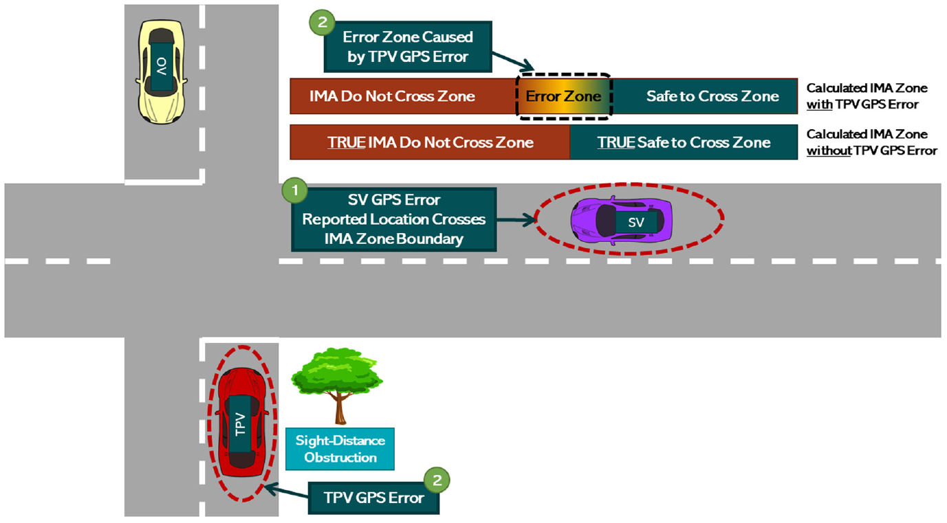
Illustration of GPS error from TPV and SV causing misclassification of IMA hazard warning.

The first error illustrated in Figure 10 shows the GPS error from the SV crossing the IMA Do Not Cross zone boundary and thus potentially reporting an SV location that is within the IMA Do Not Cross zone when its true location is outside the IMA Do Not Cross zone. The first error is also true in the reverse when the SV’s true location is within the IMA Do Not Cross zone but reports itself to be outside of the boundary because of a GPS error.

The second error illustrated in Figure 10 shows the GPS error from the TPV located at the intersection stop bar that factors into the IMA Do Not Cross boundary the calculations shown in Figure 9. The error zone shown in Figure 10 depicts the region where the boundary between the IMA Do Not Cross zone and the safe-to-cross zone may shift as a result of the TPV’s GPS error. The two sets of errors were modeled into the simulation approach to assess the impact on the performance of the TPV’s IMA safety application.

The simulation of the above scenario was conducted for a posted speed limit of 30 to 60 mph in increments of 5 mph on both the side street where the TVP starts and the major road from which the SV is approaching. The acceleration rate of the TPV is taken as 1.47 mph/sec (0.657 m/s/s) from a stopped position ( 14 ). The SV approaches the crossing point traveling at the posted speed limit. The starting location of the SV is defined in the following section. The GPS error imposed on both the TPV and SV follows the profile outlined according to SAE Standard J2945.

Implementation of SBMD in IMA Malicious Misbehavior Detection Simulation Scenario

The simulation scenario for the IMA safety application assesses the effects of vehicle malicious misbehavior on the safety application hazard warning. Figure 11 shows an illustrative example of the IMA simulated true location with three possible malicious reported locations. The simulation includes a GPS error profile for each vehicle according to SAE Standard J2945. The SBMD implementation uses the 3.6-m lateral radius and 3.5-m longitudinal radius MDE boundary reported in Table 3 at 30 m.

Figure 11.

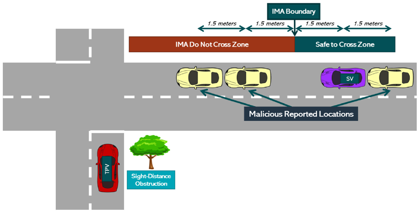
Illustration of intersection movement assist (IMA) simulated true location and malicious reported locations.

The example shown in Figure 11 above describes a scenario where the SV’s true location is located 1.5 m outside the IMA Do Not Cross zone with three possible malicious reported locations at 3 m within the IMA Do Not Cross zone, 1.5 m within the Do Not Cross zone, and 3 m outside the Do Not Cross zone.

Table 5 summarizes the list of scenarios simulated for the IMA safety application with consideration for malicious behavior.

Table 5.

Simulation Scenarios for the Intersection Movement Assist (IMA) Safety Application

Scenario	Distance from IMA crossing zone boundary
	IMA Do Not Cross zone		Boundary	IMA safe-to-cross zone
	3 m within	1.5 m within	Boundary	1.5 m outside	3 m outside
1	na	na		na	Actual
1a	na	na		Malicious
1b	na	Malicious		na
1c	Malicious	na		na
2	na	na		Actual	na
2a	na	na			Malicious
2b	na	Malicious			na
2c	Malicious	na			na
3	na	Actual		na	na
3a	na			na	Malicious
3b	na			Malicious	na
3c	Malicious			na	na
4	Actual	na		na	na
4a		na		na	Malicious
4b		na		Malicious	na
4c		Malicious		na	na

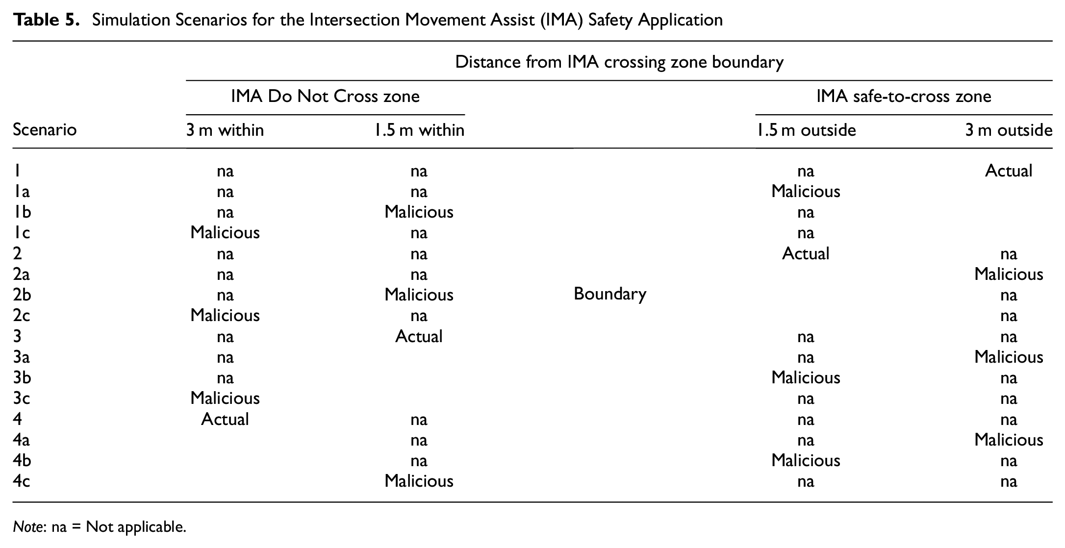
Note: na = Not applicable.

Figures 12 to 15 show a graphical illustration of the SV’s true and malicious reported locations for the IMA simulation scenarios described in Table 5. Shown in Figure 12, the scenario describes the SV’s true location at 3 m outside the IMA zone for scenario 1 (i.e., baseline application performance with no malicious behavior). For scenarios 1a, 1b, and 1c, the SV’s malicious reported locations are 1.5 m outside the IMA Do Not Cross zone, 1.5 m within the IMA Do Not Cross zone, and 3 m within the IMA Do Not Cross zone respectively.

Figure 12.

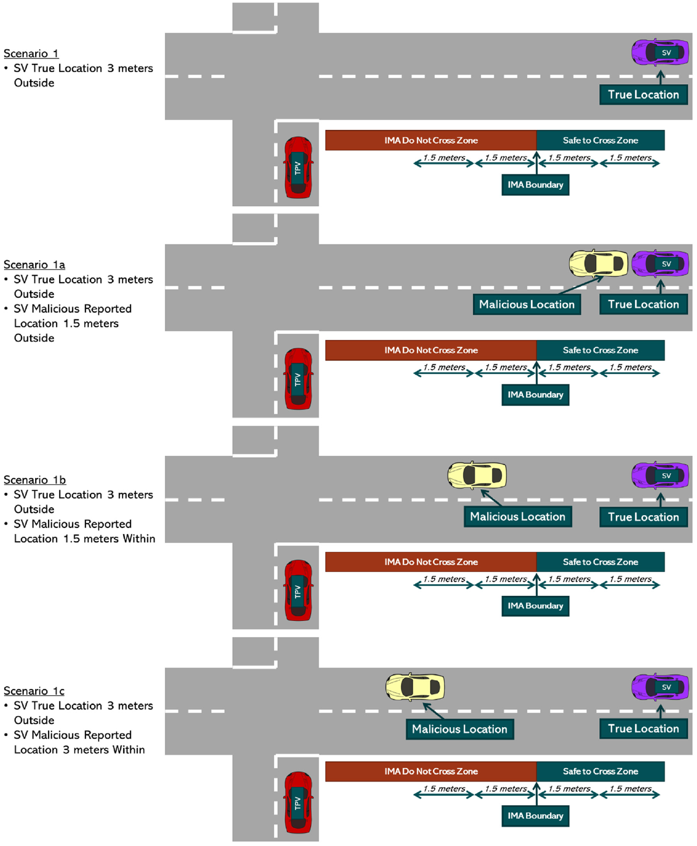
IMA scenarios 1, 1a, 1b, and 1c SV true location and malicious reported location.

Figure 13.

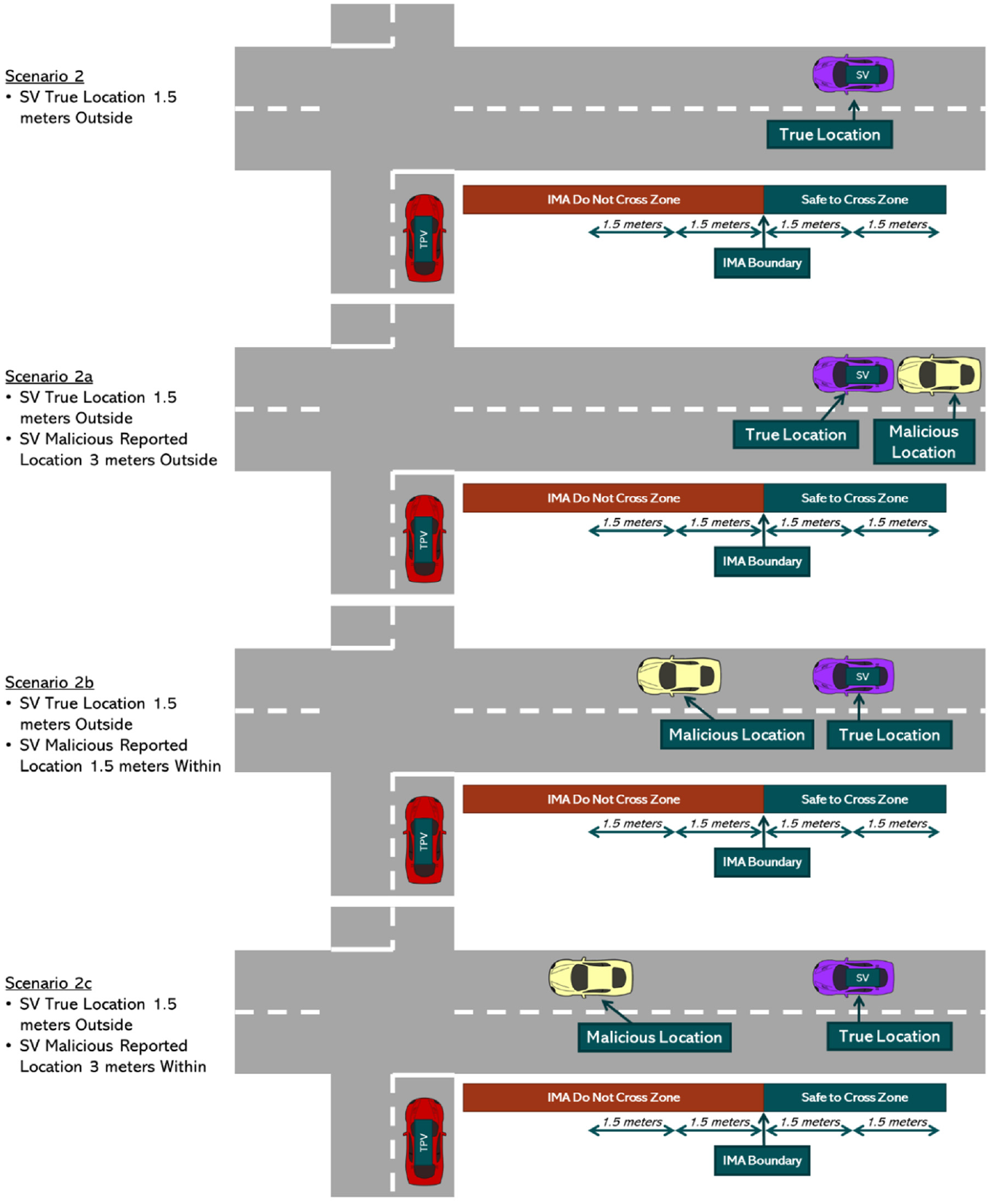
IMA Scenarios 2, 2a, 2b, and 2c SV True Location and Malicious Reported Location.

Figure 14.

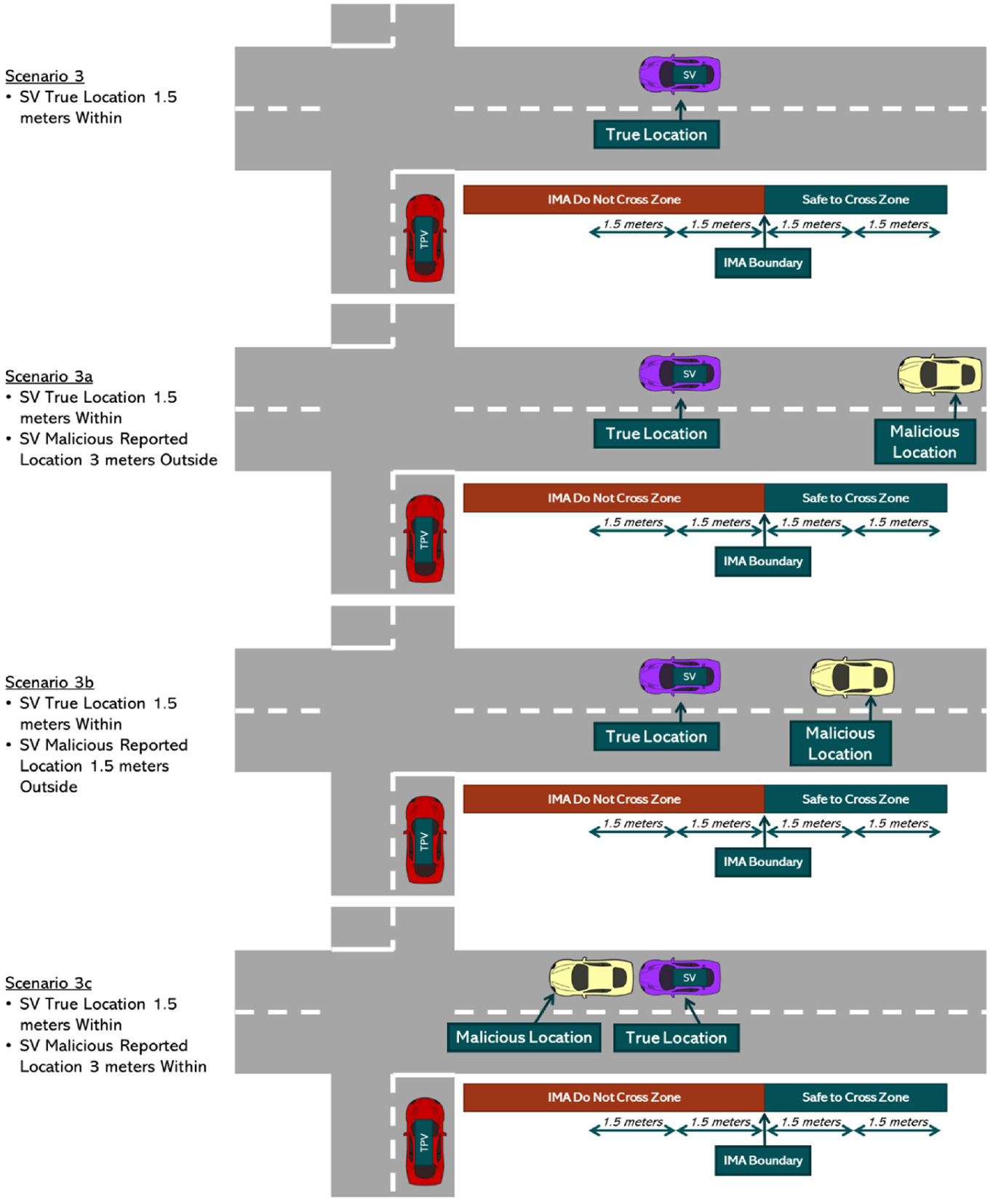
IMA scenarios 3, 3a, 3b, and 3c SV true location and malicious reported location.

Figure 15.

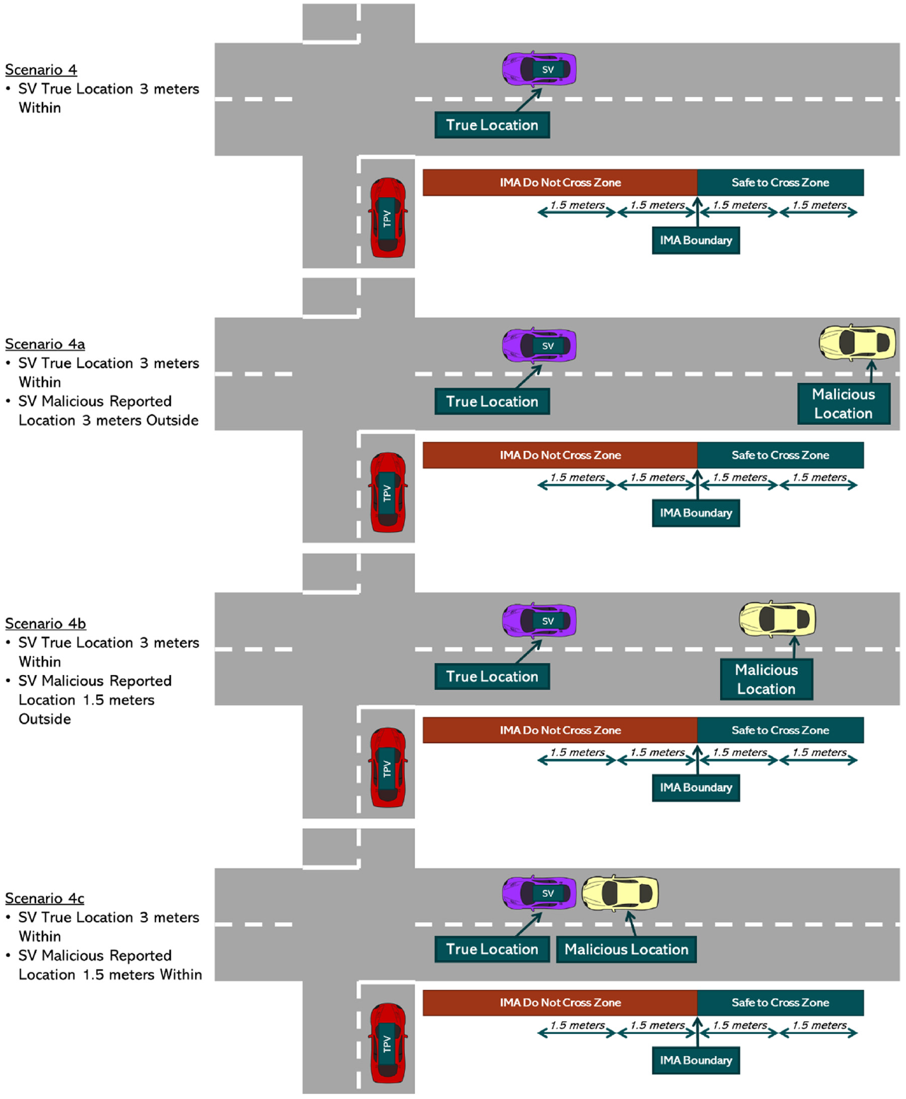
IMA scenarios 4, 4a, 4b, and 4c SV true location and malicious reported location.

Figure 13 shows the SV’s true location at 1.5 m outside the IMA zone for scenario 2 (i.e., baseline application performance with no malicious behavior). For scenarios 2a, 2b, and 2c, the SV’s malicious reported locations are 3 m outside the IMA Do Not Cross zone, 1.5 m within the IMA Do Not Cross zone, and 3 m within the IMA Do Not Cross zone respectively.

Figure 14 shows the SV’s true location at 1.5 m within the IMA zone for scenario 3 (i.e., baseline application performance with no malicious behavior). For scenarios 3a, 3b, and 3c, the SV’s malicious reported locations are 3 m outside the IMA Do Not Cross zone, 1.5 m outside the IMA Do Not Cross zone, and 3 m within the IMA Do Not Cross zone respectively.

Figure 15 shows the SV’s true location at 3 m within the IMA zone for scenario 4 (i.e., baseline application performance with no malicious behavior). For scenarios 4a, 4b, and 4c, the SV’s malicious reported locations are 3 m outside the IMA Do Not Cross zone, 1.5 m outside the IMA Do Not Cross zone, and 1.5 m within the IMA Do Not Cross zone respectively.

IMA Simulation Analysis

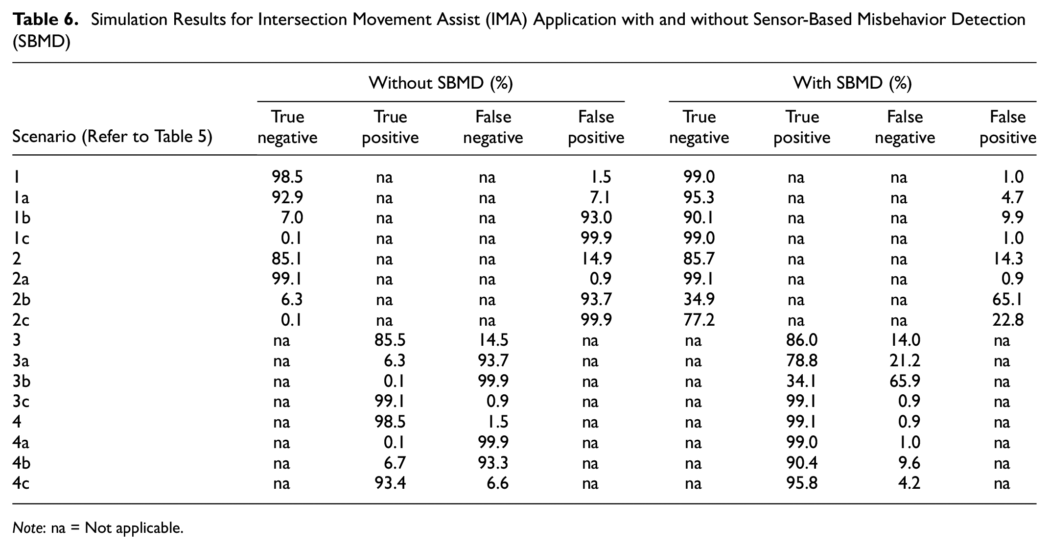
Table 6 summarizes the simulation results from the scenarios described in the previous section. A total of 100,000 random seeds for each scenario were simulated to achieve a statistically significant sample size.

Table 6.

Simulation Results for Intersection Movement Assist (IMA) Application with and without Sensor-Based Misbehavior Detection (SBMD)

Scenario (Refer to Table 5)	Without SBMD (%)				With SBMD (%)
Scenario (Refer to Table 5)	True negative	True positive	False negative	False positive	True negative	True positive	False negative	False positive
1	98.5	na	na	1.5	99.0	na	na	1.0
1a	92.9	na	na	7.1	95.3	na	na	4.7
1b	7.0	na	na	93.0	90.1	na	na	9.9
1c	0.1	na	na	99.9	99.0	na	na	1.0
2	85.1	na	na	14.9	85.7	na	na	14.3
2a	99.1	na	na	0.9	99.1	na	na	0.9
2b	6.3	na	na	93.7	34.9	na	na	65.1
2c	0.1	na	na	99.9	77.2	na	na	22.8
3	na	85.5	14.5	na	na	86.0	14.0	na
3a	na	6.3	93.7	na	na	78.8	21.2	na
3b	na	0.1	99.9	na	na	34.1	65.9	na
3c	na	99.1	0.9	na	na	99.1	0.9	na
4	na	98.5	1.5	na	na	99.1	0.9	na
4a	na	0.1	99.9	na	na	99.0	1.0	na
4b	na	6.7	93.3	na	na	90.4	9.6	na
4c	na	93.4	6.6	na	na	95.8	4.2	na

Note: na = Not applicable.

Based on the simulation analysis of the IMA safety application with malicious behavior the following is a summary of the analytical findings for the probability of misbehavior detection.

When the SV true location without malicious behavior is close to the IMA boundary, the frequency of false positive or negative hazard messages increases as a result of the influence from the IMA boundary error caused by the TPV’s GPS error.

When the malicious behavior is located further away from the IMA boundary but in the same zone as the SV’s true location, as shown in scenarios 2a and 3c, the number of false positive or negative hazard messages decreases compared with the scenarios 2 and 3 respectively without malicious behavior.

When the malicious reported location is relatively close to the SV’s true location (e.g., 1.5 m in front or behind the SV’s true location), the malicious reported location is likely still within the OV’s MDE boundary and thus is not reported as a misbehavior, so no action is taken to correct the malicious behavior.

When the malicious reported location is relatively far from the SV’s true location (e.g., more than 3 m in front or behind the SV’s true location), the malicious reported location is likely to be outside the OV’s MDE boundary and thus is reported as a misbehavior and corrective action is taken.

The results indicate a strong correlation between the increase in misbehavior detection and rectification with the distance between the SV’s true versus malicious locations. It is observed there is an increase in misbehavior detection with the increase in distance between the SV’s true and malicious reported locations. This increase in distance between the SV’s true and malicious reported locations thus increases the confidence of a malicious misbehavior detection.

Conclusion

In situations where the SV is well inside the safe-to-cross zone, SBMD only had a significant effect when the position of the SV was reported to be in the not-safe-to-cross zone. Part of the reason for this is that the application is somewhat insensitive to GPS errors, so the natural inaccuracy of GPS does not create many false alarms in this situation. The SBMD improvement in this situation was only about 0.5%. In the situations where the SV position is intentionally misrepresented as being in the not-safe-to-cross zone, the baseline (no SBMD) application exhibited a 93% false positive error. This implies that this scenario would be a good target for malicious misbehavior, since there is no real safety risk, but creating a huge number of false positive warnings would be very disruptive. As shown in Table 6, SBMD almost completely rectifies the application errors in these two cases.

The improvement afforded by SBMD in scenario 2, where the SV is somewhat closer to the boundary between safe-to-cross and not-safe-to-cross is still effective, but because of the overall position uncertainty in the vicinity of the zone boundary, the effect is only about an 80% improvement in performance.

In the hazard scenario, where the SV is actually in the not-safe-to-cross zone, SBMD produced an 80% to 99% improvement in application performance, with the greater improvements occurring when the reported position was substantially wrong. This is illustrated in Table 6.

In summary, these simulations indicate that the SBMD concept can have a substantial positive impact on the performance of the IMA application, especially under malicious attack situations.

It is important to note that, to our knowledge, these simulations represent the first rigorous treatment of the impact of errors, malicious or innocent, on overall safety application performance. It would appear beneficial to perform similar simulation on other high value applications.

The authors confirm contribution to the paper as follows: study conception and design: Scott Andrews, Dennis Fleming, Boon Teck Ong, and Saleh Mousa; data collection: Purser Sturgeon II; analysis and interpretation of results: Boon Teck Ong, Saleh Mousa, Joshua Kolleda, Jim Marousek, James Goldsmith, Mahsa Ettefagh, Diego Lodato, Scott Andrews, Dennis Fleming; draft manuscript preparation: Boon Teck Ong, Saleh Mousa, Joshua Kolleda, Jim Marousek, James Goldsmith. All authors reviewed the results and approved the final version of the manuscript.

Footnotes

Acknowledgements

The authors acknowledge Jonathan Walker (FHWA) and Steve Sill (FHWA) as the government task managers of the overall project for their feedback and oversight. The authors also acknowledge Robert Kreeb (NHTSA), Robert Heilman (NHTSA), Raymond Resendes (Volpe), Edmond Dupont (SwRI), and John Esposito (SwRI) for their extensive guidance and support throughout the execution of this task.

Declaration of Conflicting Interests

The author(s) declared no potential conflicts of interest with respect to the research, authorship, and/or publication of this article.

Author Contributions

The authors confirm contribution to the paper as follows: study conception and design: X. Author, Y. Author; data collection: Y. Author; analysis and interpretation of results: X. Author, Y. Author. Z. Author; draft manuscript preparation: Y. Author. Z. Author. All authors reviewed the results and approved the final version of the manuscript.

Funding

The author(s) disclosed receipt of the following financial support for the research, authorship, and/or publication of this article: This material is based on work conducted in supporting the Federal Highway Administration under contract number DTFH6116D00035.

ORCID iDs

Joshua Kolleda

Saleh Mousa

Scott Andrews

Dennis Fleming

Diego Lodato

James Goldsmith

Any opinions, findings, and conclusions or recommendations expressed in this publication are those of the authors and do not necessarily reflect the views of the Federal Highway Administration.

References

Liem

Murdock

Williams

Soukup

Highly Available, Self-Defending, and Malicious Fault-Tolerant Systems for Automotive Cybersecurity. Proc., IEEE 19th International Conference on Software Quality, Reliability and Security Companion (QRS-C), Sofia, Bulgaria, 2019, pp. 24–27. https://doi.org/10.1109/QRS-C.2019.00018.

Uhlemann

Introducing Connected Vehicles [Connected Vehicles]. IEEE Vehicular Technology Magazine, Vol. 10, No. 1, 2015, pp. 23–31. https://doi.org/10.1109/MVT.2015.2390920.

Parkinson

Ward

Wilson

Miller

Cyber Threats Facing Autonomous and Connected Vehicles: Future Challenges. IEEE Transactions on Intelligent Transportation Systems, Vol. 18, No. 11, 2017, pp. 2898–2915. https://doi.org/10.1109/TITS.2017.2665968.

Dehnie

Ghanadan

Methods and Systems for Detecting GPS Spoofing Attacks. Patent Number: US 8,922,427 B 2. 2014.

Mahmoud

Noureldin

Hassanein

Integrated Positioning for Connected Vehicles. IEEE Transactions on Intelligent Transportation Systems, Vol. 21, No. 1, 2020, pp. 397–409. https://doi.org/10.1109/TITS.2019.2894522.

Amoozadeh

Raghuramu

Chuah

Ghosal

Zhang

H. M.

Rowe

Levitt

Security Vulnerabilities of Connected Vehicle Streams and Their Impact on Cooperative Driving. IEEE Communications Magazine, Vol. 53, No. 6, 2015, pp. 126–132. https://doi.org/10.1109/MCOM.2015.7120028.

Gao

Coifman

Vehicle Identification and GPS Error Detection from a LIDAR Equipped Probe Vehicle. Proc., IEEE Intelligent Transportation Systems Conference, Toronto, ON, Canada, IEEE, 2006.

Peng

Hussain

Hayee

M. I.

Donath

Acquisition of Relative Trajectories of Surrounding Vehicles using GPS and SRC based V2V Communication with Lane Level Resolution. Proc., 3rd International Conference on Vehicle Technology and Intelligent Transport Systems (VEHITS 2017), Portugal, 2017, pp. 242–251.

Lim

Tuladhar

K. M.

Kim

Detecting Location Spoofing using ADAS sensors in VANETs. Proc., 16th IEEE Annual Consumer Communications & Networking Conference (CCNC), Las Vegas, 2019, pp. 1–4.

10.

Laur

M. H.

Sun

Vijayan

Schiffmann

J. K.

GPS Data Correction for Automated Vehicle. U.S. Patent Application No. 14/835,798, 2017.

11.

Ardiansyah

M. N.

An Evaluation Scheme for Assessing the Effectiveness of Intersection Movement Assist (IMA) on Improving Traffic Safety. Traffic Injury Prevention, Vol. 19, No. 2, 2018, pp. 179–183.

12.

SAE International. On-Board System Requirements for V2V Safety Communications. SAE J 2945-1-2016. SAE International, 2016.

13.

Adams

Andrews

Asudegi

Ayhan

Fisher

Fuja

Fleming

, et al. Development of DSRC Device and Communication System Performance Measures Recommendations for DSRC OBE Performance and Security Requirements. FHWA-JPO-17-483. U.S. Department of Transportation, FHWA, 2016.

14.

Geometric Design Example. University of Idaho. https://www.webpages.uidaho.edu/niatt_labmanual/chapters/geometricdesign/exampleproblems/PassingSightDistance.htm. Accessed December 10, 2019.