Macroscopic Real-Time Timetable Rescheduling Approach for High-Speed Railway under Complete Blockages Using a Three-Stage Algorithm

Abstract

The rescheduling of train timetables under a complete blockage is a challenging process, which is more difficult when timetables contain lots of trains. In this paper, a mixed integer linear programming (MILP) model is formulated to solve the problem, following the rescheduling strategy that blocked trains wait inside the stations during the disruption. When the exact end time of the disruption is known, trains at stations downstream of the blocked station can depart early. The model aims at minimizing the total delay time and the total number of delayed trains under the constraints of station capacities, activity time, overtaking rules, and rescheduling strategies. Because there are too many variables and constraints of the MILP model to be solved, a three-stage algorithm is designed to speed up the solution. Experiments are carried out on the Beijing–Guangzhou high-speed railway line from Chibibei to Guangzhounan. The original timetable contains 162 trains, including 29 cross-line trains and 133 local trains. The simulation results show that our model can handle the optimization task of the timetable rescheduling problem very well. Compared with the one-stage algorithm, the three-stage algorithm is proved to greatly improve the solving speed of the model. All instances can get a better optimized disposition timetable within 450 to 600 s, which is acceptable for practical use.

Keywords

high-speed railway disruption management timetable rescheduling linear programming

In the course of railway transportation, train operation is vulnerable to unpredictable factors such as bad weather conditions, human problems, and equipment failures. These factors may consequently lead to accidents of varying degrees, which are usually classified as disturbances or disruptions according to their impact. Under normal circumstances, the departure and arrival time of each train at each station are preset in the dispatching system, and this is called the original time.

As an accident occurs, some trains may not be able to complete the transportation task within the prescribed time because of its impact. In such cases, dispatchers will adjust the time of the affected trains to avoid delay propagation. Through their adjustments, the delay caused by a small disturbance can be recovered in a short time. However, for large disruptions, it is much more difficult for dispatchers to give a reasonable disposition timetable in a short time. In this case, an intelligent decision support system integrating optimization methods will be very useful to improve the dispatcher’s decision-making ability.

This paper focuses on the real-time timetable rescheduling problem under a complete blockage. In this scenario, all tracks in a certain segment are unavailable for trains until the disruption ends. The contributions of this paper are threefold.

First, we apply a mixed integer linear programming (MILP) model to a more complex train operation scene. In most recent studies, trains run from the same origin to the same terminus with the same stopping pattern. But in reality, different trains may have different origins, termini, and stopping patterns. Generally, if a train is late, the longer its route, the greater its resilience. But from the perspective of delay accumulation, under the same delay, a train with a longer route may accumulate more delays in its future operation. It complicates the process of timetable rescheduling. Moreover, in a railway network, there will be some cross-line trains. They may transfer the delay to other lines, causing more serious delays. In this paper, these situations are included in our scenario.

Second, when the end time of the disruption is known, we allow trains at stations downstream of the disruption to depart early to make full use of the buffer time. Zhan et al. ( 1 ) were the first to come up with this idea, and we apply their idea in our model with different constraints. A parameter $ξ$ is added in the model to describe the anticipation ability of the end time of the disruption and some new discoveries are made.

Last but not the least, a three-stage algorithm is designed to solve the MILP model. Since the MILP model may have numerous variables and constraints in our scenario, it sometimes may not be solved in a short time. Because of this, a three-stage algorithm is applied to improve the solving efficiency.

The rest of this paper is organized as follows. The next section gives an overview of the related literature. We present the problem description and the MILP model in the third section. In the fourth section, a three-stage algorithm is introduced. The fifth section presents our experimental setup and simulation results. Conclusions are drawn in the sixth section.

Literature Review

In recent years, the real-time railway rescheduling problem has been a hot topic in delay management. Cacchiani et al. ( 2 ) review the recovery models and algorithms for this problem. They conclude that the application of these models and algorithms in real-life railway systems can play an important role in increasing the quality of services. Timetable rescheduling is one of the most important research directions in the railway rescheduling problem. According to the accident type, existing studies can be divided into two categories: disturbances and disruptions. Since our focus is on disruption recovery, readers can refer to Qu et al. ( 3 ) for further reading, which reviews the methods of real-time railway traffic management under disturbances. In disruption recovery, Ghaemi et al. ( 4 ) describe the traffic level during a disruption as a bathtub with three phases: the traffic will decrease in the first phase, remain at a low level in the second phase and be restored to its original level in the third phase. Several optimization techniques are widely used to solve the three-phase traffic problem at microscopic and macroscopic levels.

At microscopic level, many studies use a detailed alternative graph model to consider the requirement of signals and switches, the headway reports, and the characterization of operations. Corman et al. ( 5 ) present a novel optimization framework for the multi-class rescheduling problem, which is designed to preserve solution quality from the higher priority classes and neglect lower priority classes. After that, they develop two heuristic algorithms to provide a set of feasible non-dominated schedules of the bi-objective rescheduling problem ( 6 ). Caimi et al. ( 7 ) embed a complex central railway station area in a closed-loop discrete-time system, to assign precomputed blocking-stairways to trains while respecting resource-based clique, connection, platform, and consistency constraints with the objective of maximizing customer satisfaction. Chu and Oetting ( 8 ) propose a microscopic method to estimate the feasibility of pre-defined dispatching measures in case of certain disruptions. Pellegrini et al. ( 9 ) develop a model in which the infrastructure is represented with fine granularity to assess the impact of the granularity of the representation of the control area. Ghaemi et al. ( 10 ) extend it with the short-turning measures that trains approaching the blockage cannot proceed according to their original plans and have to short-turn at a station close to the disruption on both sides. Because of the magnitude of the model details, these microscopic models can only deal with the work of relatively small areas.

To improve the efficiency of decision-making, many scholars have begun to use an event–activity network to formulate the train operations, without taking signals and switches into account. Veelenturf et al. ( 11 ) propose an integer linear programming (ILP) model to handle large-scale disruptions at a macroscopic level by adjusting the departure and arrival time of trains at stations. Meng and Zhou ( 12 ) propose a stochastic programming model for single-track railway lines that takes the uncertainty of the disruption duration into account. Their model reschedules the timetable dynamically by a rolling horizon approach. Louwerse and Huisman ( 13 ) present a MILP model suitable for a partial and a complete blockage and based on Netherlands Railways. Measures of delaying trains, canceling trains, and reversing trains at stations adjacent to the blockage are taken to reschedule trains. Zhan et al. ( 1 ) also formulate a MILP model to arrange for the affected trains to stop at stations during a disruption and produce a disposition timetable for trains to resume operation after the disruption, considering headway and station capacity constraints. After that, they extend their model to a case of a partial segment blockage and compare three practical train rescheduling strategies based on a real-world instance in China ( 14 ). To reduce passenger inconveniences during disruptions, Binder et al. ( 15 ) integrate passenger rerouting and timetable rescheduling into an ILP model where limited vehicle capacity is taken into account. Ghaemi et al. ( 16 ) consider the interaction of traffic on both sides of the blockage and apply a MILP model to find the optimal short-turning solutions. In their model, blocked trains can return to their origin station by taking over train services in the opposite direction. Zhu and Goverde ( 17 ) propose a MILP model where more short-turn station candidates and more stopping patterns are given for each train. From their test results, these macroscopic models can solve the rescheduling problem of a large-scale disruption very well, and still take plenty of time to get an optimal timetable when there are too many trains needing to be adjusted.

Most of the studies above are tested on lines with a few trains or select part of the all-day timetable to simulate. When facing a line with lots of trains or an all-day timetable, their methods may not give feasible results in a short time. Some European scholars have recently tried to use short-turning measures to narrow the scope of the disruption ( 10 , 16 , 17 ), except for Meng et al. ( 12 ) and Zhan et al. ( 1 , 14 ). In Meng et al. ( 12 ) and Zhan et al. ( 1 , 14 ), their test lines are railway lines in China, where trains operate with seat reservations for passengers. After passing their origins, they must continue to their termini and cannot return to their origin by taking over the passenger services in the opposite direction. Because of the train seats having been sold in advance, the cancelation of trains will result in major changes of passenger itineraries. In this paper, we extend the mathematical model originally described by Zhan et al. ( 1 ) and the timetable is only rescheduled by retiming and reordering measures. Our model is built to solve the three-phase traffic problem of an all-day timetable at once. Because we do not use short-turning and canceling measures, coupled with numerous trains operating on our test line, the scope of a disruption will be wider. So we propose four new strategies to reschedule trains and a brand-new three-stage algorithm to accelerate the solving speed. Simulations are carried out on the Beijing–Guangzhou high-speed railway line with 29 cross-line trains and 133 local trains.

Problem Description and Model Formulation

Problem Description

During railway operation, the performance of infrastructure will be affected by unexpected factors. When the facilities in one or more segments cannot guarantee the safe passage of trains, it will cause a disruption. If a complete blockage occurs, trains cannot pass through the blocked segment until the blockage is completely repaired. The affected trains have to stop at a nearby station during the disruption.

It should be noted that the high-speed railway line we consider here has two tracks in each segment, with one track for each direction. Trains in different directions run independently in each segment. In China, we call the train going away from Beijing the “down train” and the train in the opposite direction the “up train”; up trains are numbered even and down trains are numbered odd. In this paper, down trains are taken as our rescheduling object.

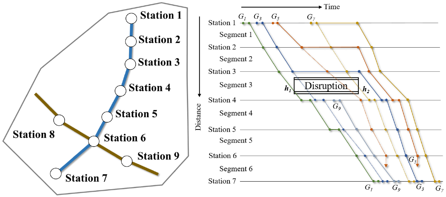
An example of this problem is shown in Figure 1. The blue line consists of seven stations and six segments. In particular, station 6 is a hub station where trains can run to another line. Five trains are running on it during the blockage, with the same high speed. $G_{1}, G_{3}, G_{7}$ are local trains from station 1 to station 7, while $G_{9}$ is a local train from station 4 to station 7. $G_{5}$ is a cross-line train from station 6 to another line. Assume that segment 3 is blocked at time $h_{1}$ and is completely repaired at time $h_{2}$ . To minimize the blockage impact on rail services, dispatchers need to provide a reasonable stopping plan for blocked trains during the disruption and a new timetable for service resumption. In this example, each station has one track; the dotted lines and the solid lines respectively represent the timetable before and after the adjustment.

Figure 1.

An example of train dispatching under a complete blockage.

Model Formulation

Assumptions

In the case of complete blockages, rescheduling the train timetable is a complicated process. To simplify the problem modeling, some assumptions are made, which do not affect the problem generality.

Before the disruption occurs, trains operate according to the original timetable. The event time is specified in minutes.

When a disruption occurs, trains that have entered the blocked segment can pass as planned.

After the disruption occurs, each track in stations for the down/up direction can be used by each down/up train, and each track has at least one platform for passengers to alight/board.

Methods of canceling trains will not be taken into account. The original timetable will be retimed and reordered to minimize train delays.

The origin and terminus of the railway line have enough tracks for trains to operate.

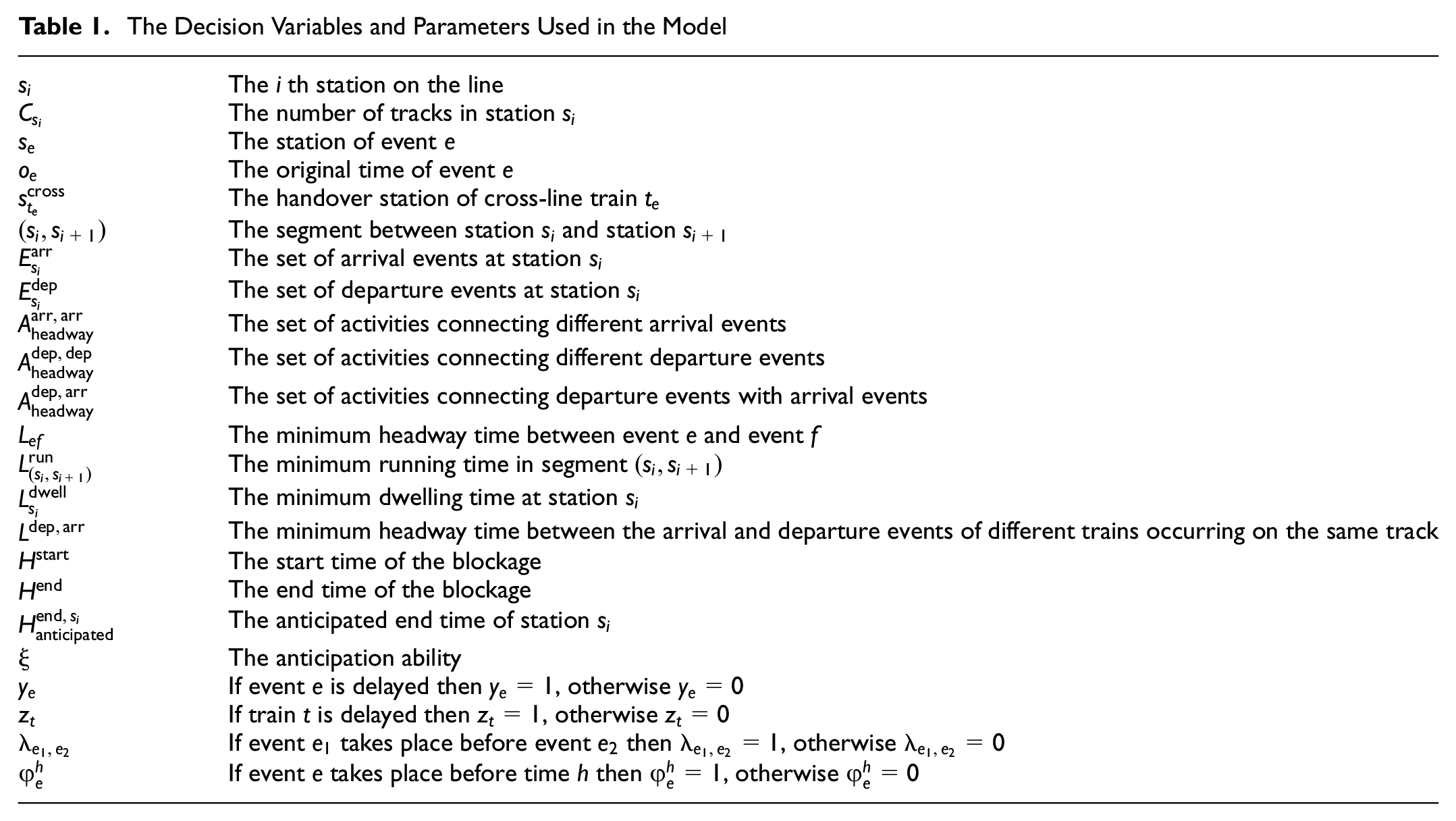
For a better understanding of this paper, the decision variables and parameters are listed in Table 1.

Table 1.

The Decision Variables and Parameters Used in the Model

$s_{i}$	The $i$ th station on the line
$C_{s_{i}}$	The number of tracks in station $s_{i}$
$s_{e}$	The station of event $e$
$o_{e}$	The original time of event $e$
$s_{t_{e}}^{cross}$	The handover station of cross-line train $t_{e}$
$(s_{i}, s_{i + 1})$	The segment between station $s_{i}$ and station $s_{i + 1}$
$E_{s_{i}}^{arr}$	The set of arrival events at station $s_{i}$
$E_{s_{i}}^{dep}$	The set of departure events at station $s_{i}$
$A_{headway}^{arr, arr}$	The set of activities connecting different arrival events
$A_{headway}^{dep, dep}$	The set of activities connecting different departure events
$A_{headway}^{dep, arr}$	The set of activities connecting departure events with arrival events
$L_{ef}$	The minimum headway time between event $e$ and event $f$
$L_{(s_{i}, s_{i + 1})}^{run}$	The minimum running time in segment $(s_{i}, s_{i + 1})$
$L_{s_{i}}^{dwell}$	The minimum dwelling time at station $s_{i}$
$L^{dep, arr}$	The minimum headway time between the arrival and departure events of different trains occurring on the same track
$H^{start}$	The start time of the blockage
$H^{end}$	The end time of the blockage
$H_{anticipated}^{end, s_{i}}$	The anticipated end time of station $s_{i}$
$ξ$	The anticipation ability
$y_{e}$	If event $e$ is delayed then $y_{e} = 1$ , otherwise $y_{e} = 0$
$z_{t}$	If train $t$ is delayed then $z_{t} = 1$ , otherwise $z_{t} = 0$
$λ_{e_{1}, e_{2}}$	If event $e_{1}$ takes place before event $e_{2}$ then $λ_{e_{1}, e_{2}} = 1$ , otherwise $λ_{e_{1}, e_{2}} = 0$
$φ_{e}^{h}$	If event $e$ takes place before time $h$ then $φ_{e}^{h} = 1$ , otherwise $φ_{e}^{h} = 0$

Model Basics

The train rescheduling problem can be formulated by an event–activity network, with $N = (E, A)$ . In the network, event $e$ ( $e \in E$ ) may be an arrival or a departure event of a train at a station. An activity ( $a$ ) is the connection between two different events. For the sake of argument, the rescheduled time of event $e$ is marked as $x_{e}$ and the original time of the event $e$ is marked as $o_{e}$ . Let $S$ be the set of stations and $T$ be the set of trains. $t_{e}$ means the train of event $e$ . Stations and trains are numbered in the order of their occurrences. $E_{s_{i}}^{arr}$ and $E_{s_{i}}^{dep}$ respectively represent the arrival and departure event set of station $s_{i}$ . The activity set $A$ is divided into two subsets. One subset $A_{train}$ includes activities between the departure event and the arrival event of one train. Another subset $A_{headway}$ includes activities that connect events of different trains.

In addition, the segment ( $s_{k}$ , $s_{k + 1}$ ) is taken as the location of the blockage. We assume that the blockage lasts from $H^{start}$ to $H^{end}$ . The following decision variables $y_{e}$ and $z_{t}$ are introduced to indicate whether event $e$ is delayed and whether train $t$ is delayed:

y_{e} = {\begin{matrix} 1 & if event e \in E is delayed \\ 0 & otherwise \end{matrix}

(1)

z_{t} = {\begin{matrix} 1 & if train t \in T is delayed \\ 0 & otherwise \end{matrix}

(2)

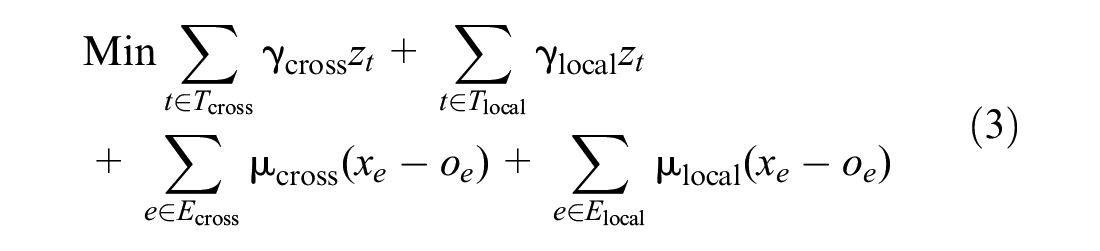
Two types of penalties are introduced to adjust the impact on delayed train numbers and the total delay time. The parameter $γ$ represents the penalty for the number of delayed trains and the parameter $μ$ represents the penalty for the total delay time. Subscripts “ $cross$ ” and “ $local$ ” denote cross-line and local trains.

The basic model of the timetable rescheduling problem is as follows:

\begin{matrix} Min \sum_{t \in T_{cross}} γ_{cross} z_{t} + \sum_{t \in T_{local}} γ_{local} z_{t} \\ + \sum_{e \in E_{cross}} μ_{cross} (x_{e} - o_{e}) + \sum_{e \in E_{local}} μ_{local} (x_{e} - o_{e}) \end{matrix}

(3)

subject to

0 \leq x_{e} - o_{e} \forall e \in E

(4)

1 - M_{1} (1 - y_{e}) \leq x_{e} - o_{e} \leq M_{1} y_{e} \forall e \in E

(5)

x_{e} \geq H^{end} \forall e \in E_{s_{k}}^{dep} : H^{start} < o_{e} \leq H^{end}

(6)

x_{e} = o_{e}, y_{e} = 0 \forall e \in E : o_{e} \leq H^{start}

(7)

z_{t} - y_{e} \geq 0 \forall t \in T, e \in E_{t}

(8)

y_{e}, z_{t} \in {0, 1}, x_{e} \in N^{*}

(9)

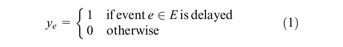
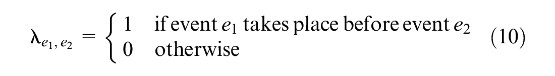
The objective function Formula 3 minimizes the number of delayed trains and the total delay time. Formula 4 ensures that any event cannot occur before its original time. Formula 5 ensures the relationship between the binary variable $y_{e}$ and the rescheduled time of event $e$ . The parameter $M_{1}$ is a large number to limit the maximum deviation between the rescheduled time and the original time. Formula 6 means that no train can pass the blocked segment during the blockage. Formula 7 indicates that trains run at the original time before the blockage. Formula 8 denotes that if one of the events of train $t$ is delayed, train $t$ is delayed. Formula 9 specifies the domains of decision variables.

Additional Constraints

To ensure the safety of passenger services, more constraints need to be added. These constraints can be divided into four categories, namely station capacity constraints, activity time constraints, overtaking rule constraints, and rescheduling strategy constraints. Recall that we extend the model in Zhan et al. ( 1 ), using the same constraints of activity time, train overtaking, and station capacity. We propose four rescheduling strategies based on complex scenarios, and brand-new strategy constraints are added in our model.

Station Capacity Constraints

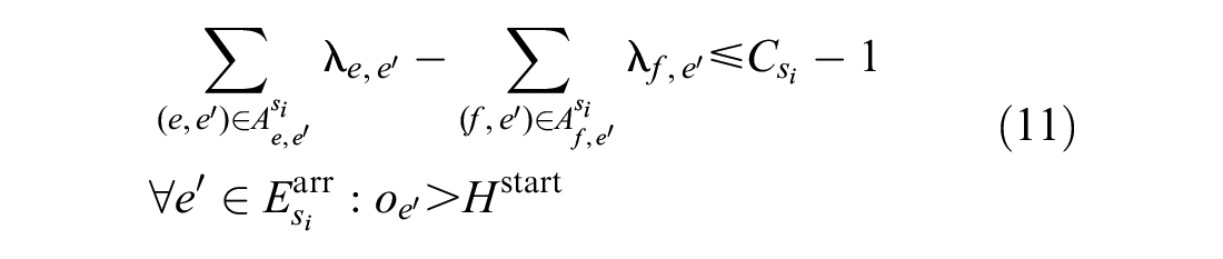
Suppose train $t$ is heading for station $s_{i}$ . In order for train $t$ to enter station $s_{i}$ smoothly, station $s_{i}$ must have at least one track for train $t$ to stop or pass. This means that before train $t$ arrives, the number of trains dwelling at station $s_{i}$ must be less than the track number of station $s_{i}$ . To record the number of trains in station $s_{i}$ , the following binary variable is introduced to describe the sequence of two events $e_{1}, e_{2}$ :

λ_{e_{1}, e_{2}} = {\begin{matrix} 1 & if event e_{1} takes place before event e_{2} \\ 0 & otherwise \end{matrix}

(10)

By comparing the arrival time of train $t$ at station $s_{i}$ with other trains’ arrival and departure time at station $s_{i}$ , the number of trains at station $s_{i}$ before train $t$ arrives can be calculated as $\sum_{(e, e') \in A_{e, e'}^{s_{i}}} λ_{e, e'} - \sum_{(f, e') \in A_{f, e'}^{s_{i}}} λ_{f, e'}$ . $A_{e, e'}^{s_{i}}$ represents the set of activities that connect the arrival event $e$ of any other train with the arrival event $e'$ of train $t$ at station $s_{i}$ . $A_{f, e'}^{s_{i}}$ represents the set of activities that connect the departure event $f$ of any other train with the arrival event $e'$ of train $t$ at station $s_{i}$ . In addition, the train of event $f$ is the same train as that of event $e$ . Let the number of tracks in station $s_{i}$ be $C_{s_{i}}$ . Therefore, we can obtain the following station capacity constraints:

\begin{matrix} \sum_{(e, e') \in A_{e, e'}^{s_{i}}} λ_{e, e'} - \sum_{(f, e') \in A_{f, e'}^{s_{i}}} λ_{f, e'} \leq C_{s_{i}} - 1 \\ \forall e' \in E_{s_{i}}^{arr} : o_{e'} > H^{start} \end{matrix}

(11)

Activity Time Constraints

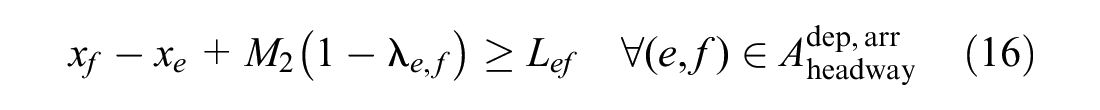
These constraints include minimum operating time constraints and minimum headway time constraints. Formulas 12 to 16 are added to the model.

x_{f} - x_{e} \geq L_{ef} \forall (e, f) \in A_{train}

(12)

x_{f} - x_{e} + M_{2} (1 - λ_{e, f}) \geq L_{ef}

\forall (e, f) \in A_{headway}^{arr, arr}, A_{headway}^{dep, dep}

(13)

λ_{e, f} + λ_{f, e} = 1 \forall (e, f) \in A_{headway}^{arr, arr}, A_{headway}^{dep, dep}

(14)

x_{e} - x_{f} + M_{2} λ_{e, f} \geq - L_{ef} + 1 \forall (e, f) \in A_{headway}^{dep, arr}

(15)

x_{f} - x_{e} + M_{2} (1 - λ_{e, f}) \geq L_{ef} \forall (e, f) \in A_{headway}^{dep, arr}

(16)

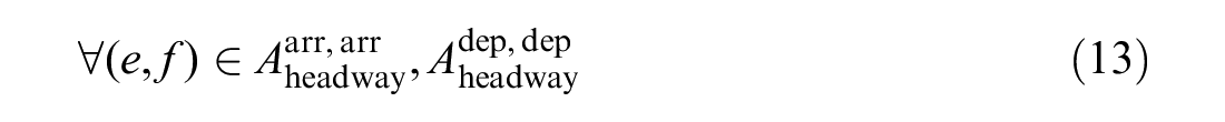
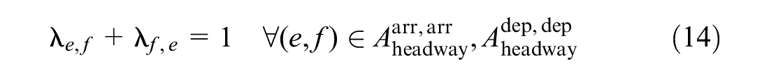
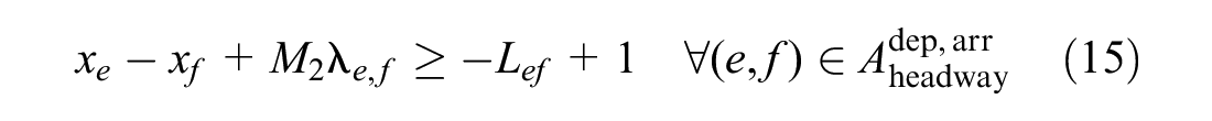
Formula 12 ensures that any train meets minimum operating time constraints. If event $e$ is a departure event at station $s_{i}$ and event $f$ is an arrival event at station $s_{i + 1}$ , $L_{ef}$ is the value of the minimum running time of segment $(s_{i}, s_{i + 1})$ , which is denoted as $L_{(s_{i}, s_{i + 1})}^{run}$ . If event $f$ and event $e$ are the departure and arrival events at station $s_{i}$ , $L_{ef}$ is the value of the minimum dwelling time at station $s_{i}$ , which is denoted as $L_{s_{i}}^{dwell}$ . Formulas 13 to 14 represent that activities between the arrival/departure events of any two trains must meet the minimum headway time. $λ_{e, f}$ is the binary variable introduced in the previous section. $M_{2}$ is a large number that makes Formulas 13, 15, and 16 true, when event $e$ occurs after event $f$ . Formulas 15 to 16 restrict the activity time between departure and arrival events on the same track. In Formulas 15 to 16, event $f$ is an arrival event of one train and event $e$ is a departure event of another train. $L_{ef}$ is the minimum headway time between the arrival and departure events of different trains occurring on the same track, which is denoted as $L^{dep, arr}$ .

Train Overtaking Constraints

As mentioned earlier, there is only one track in segments for trains running in the same direction. One train can only overtake another train at a station, not in a segment. To meet this requirement, the constraints on train overtaking are as follows:

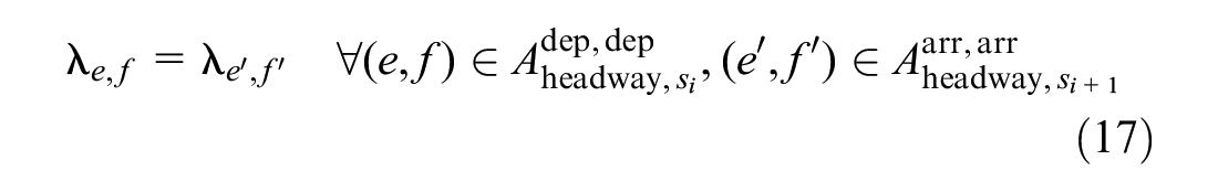
λ_{e, f} = λ_{e', f'} \forall (e, f) \in A_{headway, s_{i}}^{dep, dep}, (e', f') \in A_{headway, s_{i + 1}}^{arr, arr}

(17)

Formula 17 means that the order in which two trains arrive at the next station must be the same as the order in which they leave the previous station. It should be noted that $t_{e} = t_{e'}$ , $t_{f} = t_{f'}$ , and $A_{headway, s_{i}}$ is the set of activities that connect events of different trains at station $s_{i}$ .

Rescheduling Strategy Constraints

We set four strategies to reschedule trains. First of all, make blocked trains stop at stations as much as possible and avoid them staying in segments for too long. So during the rescheduling process, we set the maximum running time of the trains in each segment to the planned running time in their original timetable. Although this measure will increase the total delay time, it will better ensure the safety of passengers. Note that, in dense traffic lines, not all trains can meet this limit. A special case is shown in Figure 2, which shows a part of the timetable used in this paper. At the beginning of the blockage, three trains enter the segment between station 11 and station 12. 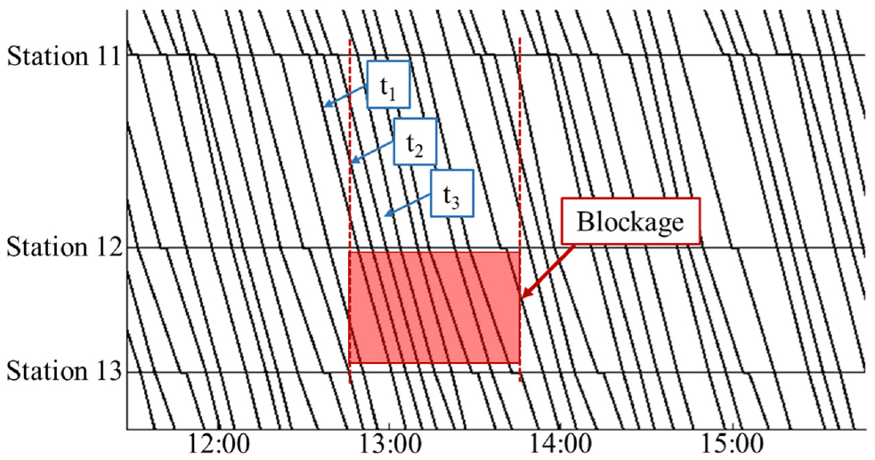Since there are only two tracks in station 12 for trains to stop, train $t_{3}$ cannot stop at station 12 and must stay in the segment until the blockage is over. If this happens at the start time of the disruption, it is impossible for all trains to meet the maximum running time limit. Only in this case will we allow these extra trains to run slowly or even stop in the segment, without setting the maximum running time limit.

Figure 2.

A special case that not all trains running in one segment can stop at the stations ahead.

Second, blocked trains at stations downstream of the blocked segment can depart early when the end time of the disruption is known. In reality, the end time is uncertain at the beginning, but we can get it in advance before the disruption is over. We introduce a parameter $ξ$ to describe the anticipation ability. For example, $ξ = 5$ means that the end time of the disruption is obtained at 5 min before its end. When the disruption ends, trains stopping at station $s_{k}$ will depart and at least one track will be available. So trains at stations $s_{i} (i < k)$ can depart early, freeing up their tracks for rearward trains. The anticipated end time of each station can be obtained as follows:

H_{anticipated}^{end, s_{i}} = {\begin{matrix} H^{end} & if i = k \\ H^{end} - ξ & if i < k \end{matrix}

(18)

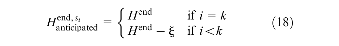
At the anticipated end time, blocked trains are allowed to leave their stations for the next one, utilizing these early departure times to resume normal operations more quickly.

Third, before the disruption is completely repaired, a delayed train cannot affect the subsequent punctual trains. If train $t$ arrives at station $s_{i}$ and there are tracks available for stopping in station $s_{i + 1}$ , there are two options for train $t$ . One is to leave station $s_{i}$ on time, and the other is to stay at station $s_{i}$ and let other trains overtake. So if train $t$ chooses to stay at station $s_{i}$ , it cannot leave station $s_{i}$ until the anticipated end time to decrease its impact on other punctual trains. To implement this strategy, we need to know the number of trains dwelling at a station and the number of trains running in a segment at any given time. Therefore, we introduce another binary variable as

φ_{e}^{h} = {\begin{matrix} 1 & if event e takes place before time h \\ 0 & otherwise \end{matrix}

(19)

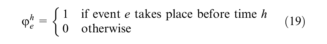
Formulas 20 to 21 represents the constraints of variable $φ_{e}^{h}$ .

h - x_{e} + M_{2} (1 - φ_{e}^{h}) \geq 1 e \in E

(20)

x_{e} - h + M_{2} φ_{e}^{h} \geq 0 e \in E

(21)

Formulas 22 to 24 are added to the downstream stations of the blocked segment to meet the third strategy.

\begin{matrix} \sum_{f \in E_{s_{i}}^{dep *}} φ_{f}^{H_{anticipated}^{end, s_{i}}} - \sum_{e \in E_{s_{i + 1}}^{arr} : t_{e} = t_{f}} φ_{e}^{H_{anticipated}^{end, s_{i + 1}}} \\ + \sum_{e' \in E_{s_{i + 1}}^{arr} : t_{e'} = t_{f'}} φ_{e'}^{H_{anticipated}^{end, s_{i + 1}}} \\ - \sum_{f' \in E_{s_{i + 1}}^{dep}} φ_{f'}^{H_{anticipated}^{end, s_{i + 1}}} \leq C_{s_{i + 1}} \\ \forall i \in [1, k - 1]; E_{s_{i + 1}}^{dep} = {f' | H^{start} < o_{f'} < H_{anticipated}^{end, s_{i + 1}}}; \end{matrix}

E_{s_{i}}^{dep *} = {f | H^{start} < o_{f} < H_{anticipated}^{end, s_{i}} \ s_{t_{f}}^{cross} = s_{i}}

(22)

φ_{f}^{H_{anticipated}^{end, s_{i}}} = 1 - y_{f}

\forall f \in E_{s_{i}}^{dep} : H^{start} < o_{f} < H_{anticipated}^{end, s_{i}}

(23)

y_{f'} \geq y_{e} \forall e \in E_{s_{i}}^{arr} : H^{start} < o_{e} < H_{anticipated}^{end, s_{i}},

f' \in E_{s_{i - 1}}^{dep} : t_{e} = t_{f'}

(24)

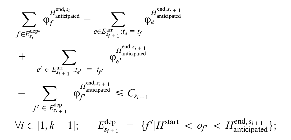
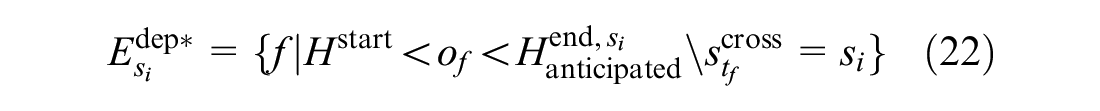
Formula 22 ensures that before the blockage ends, one of the affected trains can leave its current station only when at least one track is free at the next station. In Formula 22, $\sum_{f \in E_{s_{i}}^{dep *}} φ_{f}^{H_{anticipated}^{end, s_{i}}} - \sum_{e \in E_{s_{i + 1}}^{arr} : t_{e} = t_{f}} φ_{e}^{H_{anticipated}^{end, s_{i + 1}}}$ represents the number of trains running in the segment $(s_{i}, s_{i + 1})$ during the blockage. $\sum_{e' \in E_{s_{i + 1}}^{arr} : t_{e'} = t_{f'}} φ_{e'}^{H_{anticipated}^{end, s_{i + 1}}} - \sum_{f' \in E_{s_{i + 1}}^{dep}} φ_{f'}^{H_{anticipated}^{end, s_{i + 1}}}$ represents the number of trains waiting in station $s_{i + 1}$ during the blockage. It should be noted that $s_{t_{f}}^{cross}$ represents the handover station of train $t_{f}$ and $E_{s_{i}}^{dep *}$ does not include the departure events of the cross-line trains departing from station $s_{i}$ to another line. Formula 23 denotes that if departure event $f$ occurs before time $H_{anticipated}^{end, s_{i}}$ , event $f$ must be on time; otherwise, the departure event $f$ must be delayed. Formula 24 denotes that if the departure event $f'$ of a train occurs on time, its arrival event $e$ at the next station must also occur on time.

Last but not the least, to avoid delay propagation, those cross-line trains that arrive at their handover stations on time during the rescheduling process must be sent to other lines on time. Formula 25 ensures that the fourth strategy is met.

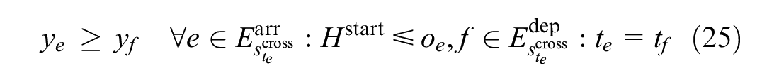
y_{e} \geq y_{f} \forall e \in E_{s_{t_{e}}^{cross}}^{arr} : H^{start} \leq o_{e}, f \in E_{s_{t_{e}}^{cross}}^{dep} : t_{e} = t_{f}

(25)

This ensures that when $y_{e}$ is equal to 0, $y_{f}$ must be 0 as well, and when $y_{f}$ is equal to 1, $y_{e}$ must be 1.

Valid Constraints

When a train departs from a station before a certain point in time, its arrival event at that station must also occur before that point in time. Accordingly, when a train arrives at a station after a certain point in time, its departure event at that station will also occur after that point in time. Although these constraints are implied in the above constraints, we explicitly add these constraints here to strengthen the formulation, which helps us to improve the solution speed. These constraints are as follows.

\begin{matrix} λ_{e, e'} \geq λ_{f, e'} \forall e' \in E_{s_{i}}^{arr} : o_{e'} > H^{start} \\ e \in E_{s_{i}}^{arr} : t_{e} = t_{f}, f \in E_{s_{i}}^{dep} : o_{f} > H^{start}, t_{e'} \neq t_{e} \end{matrix}

(26)

\begin{matrix} φ_{e}^{H_{anticipated}^{end, s_{i}}} \geq φ_{f}^{H_{anticipated}^{end, s_{i}}} \\ \forall e \in E_{s_{i}}^{arr} : H^{start} < o_{e} < H_{anticipated}^{end, s_{i}}, f \in E_{s_{i}}^{dep} : t_{f} = t_{e} \end{matrix}

(27)

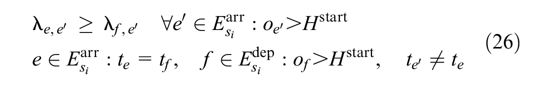
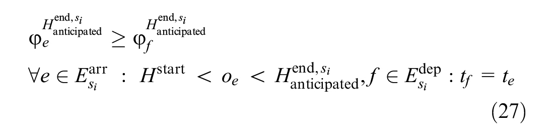
Formula 26 is added in each station and Formula 27 is added in the downstream stations of the blocked segment. In Formula 26, if $λ_{e, e'} = 0$ , which means that train $t_{e}$ arrives at station $s_{i}$ after $t_{e'}$ arrives at station $s_{i}$ , $λ_{f, e'}$ must be 0. If $λ_{f, e'} = 1$ , which means that train $t_{f}$ leaves station $s_{i}$ before $t_{e'}$ arrives at station $s_{i}$ , $λ_{e, e'}$ must be 1. The same is true in Formula 27.

Three-Stage Algorithm

Because of the excessive number of trains in a day, having too many variables and constraints in the model makes it difficult to solve. Thus, how to improve the solving ability of the model becomes another focus of this paper.

Source of Ideas

When a disruption occurs, many events need to be rescheduled. If the number of trains that need to be rescheduled can be reduced, it will have a positive influence on the solution of the problem. Let us imagine the worst situation, that dispatchers do not make any adjustments under a disruption. Under this situation, trains may still operate according to the fixed order in their original timetable. Following this rule, a feasible timetable can be obtained, whereby delayed trains can be extracted for optimization. Because it is the worst situation and the delay is propagated backward from train to train, the optimization of these delayed trains will mitigate the impact of delays and reduce the number of delayed trains. This means that the optimization result may only have a slight influence on those punctual trains in the feasible timetable. So we can merge the optimized timetable of delayed trains with the feasible timetable of punctual trains to get the disposition timetable. In this way, the original large-scale problem is simplified into a small-scale problem, and finally solved by optimizing the small-scale problem.

Computational Procedure

According to the above description, a three-stage algorithm is built. The overall process of the three-stage algorithm is shown in Figure 3.

Figure 3.

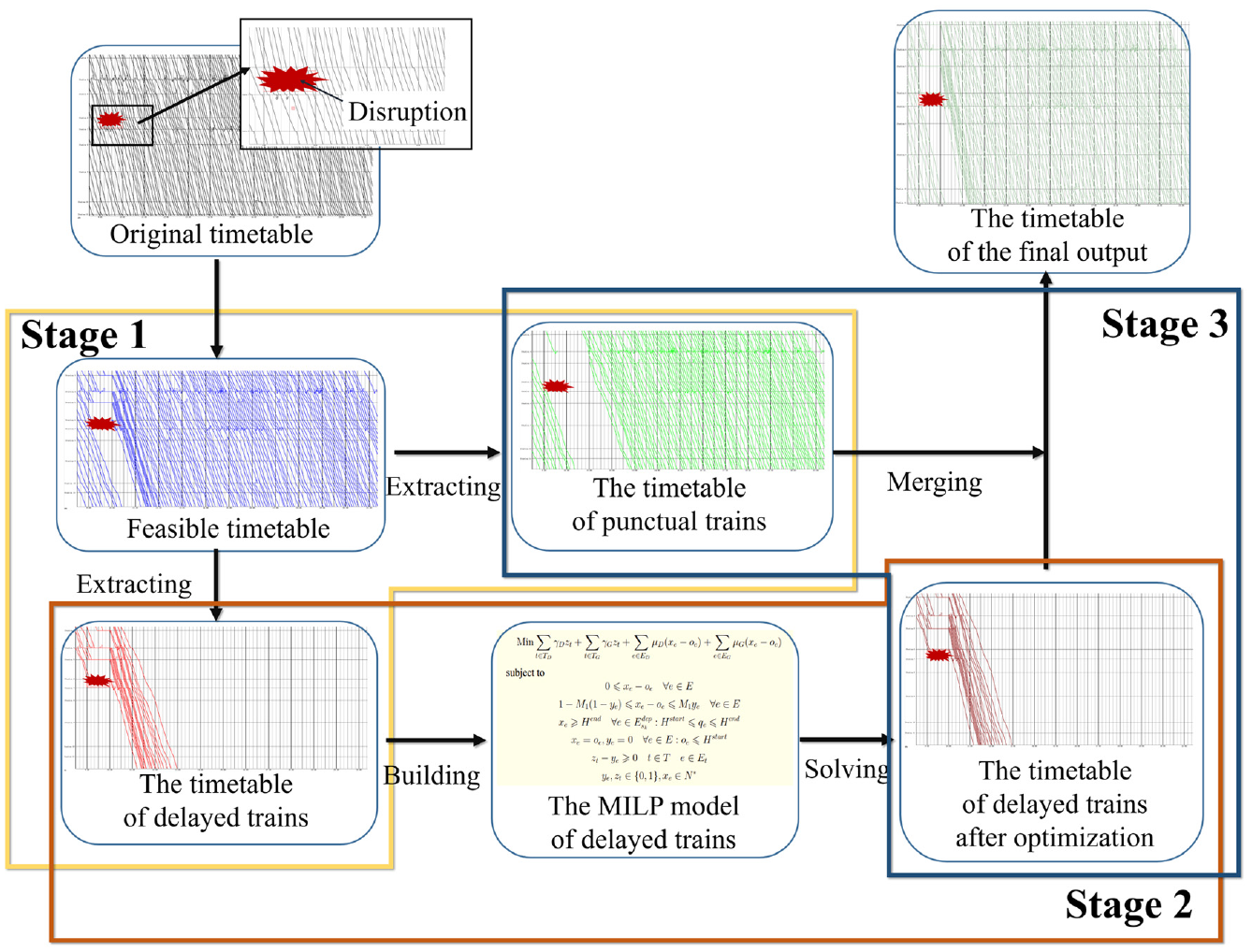
The flow chart of the three-stage algorithm.

Stage 1: Generate a Feasible Timetable to Extract Delayed Trains

In Stage 1, to generate a feasible timetable, activity time constraints and station capacity constraints need to be met. Our goal is to allocate the event time according to the fixed order in the original timetable. Figure 4 gives the flow chart of the algorithm, which takes six steps.

Figure 4.

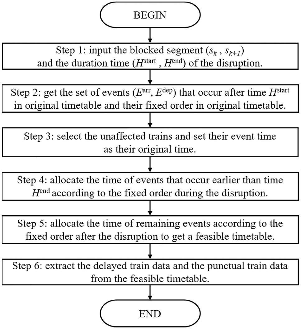
The generating algorithm in Stage 1.

Assume that the terminus of the line is station $s_{n}$ and the blocked segment is segment ( $s_{k}$ , $s_{k + 1}$ ). The minimum headway time between arrival events is denoted as $L^{arr, arr}$ and the minimum headway time between departure events is denoted as $L^{dep, dep}$ . In the generating algorithm, Steps 1, 2, and 6 are easy to understand. The unaffected trains in Step 3 include trains that have entered or passed through the blocked section before the beginning of the disruption, as well as trains from the upstream station of station $s_{k}$ , such as $G_{1}$ and $G_{9}$ in Figure 1.

Step 4 allocates event time from station $s_{k}$ to station $s_{1}$ to simulate the process of arranging train stops. At this step, only station capacity constraints (Formula 11) need to be considered. Each station can only accommodate up to the same number of trains as its track number. From station $s_{k}$ to station $s_{1}$ , station tracks are used for train stops and only when the current station’s tracks are all occupied, the next downstream station’s tracks can be used. In this step, if a train needs to stop at a station during the disruption, the time of its events before the departure event at this station needs to be set to their original time.

Let us take $G_{3}$ , $G_{5}$ , and $G_{7}$ in Figure 1 as examples. From station 3 to station 1, three trains stop in sequence according to the fixed arrival order. As shown in Figure 1, $G_{3}$ needs to stop at station 3, $G_{5}$ needs to stop at station 2, and $G_{7}$ needs to stop at station 1. Therefore, the time of the events of $G_{3}$ before its departure event at station 3, the events of $G_{5}$ before its departure event at station 2, and the events of $G_{7}$ before its departure event at station 1 are set to their original times. The time of the remaining events will be set in Step 5.

Step 5 allocates the time of all remaining events from station $s_{1}$ to station $s_{n}$ by meeting activity time constraints (Formulas 12–14) and station capacity constraints (Formula 11). For each station, we have three procedures: first set the time of arrival events, then set the time of departure events, and finally adjust the setting time of arrival and departure events.

Continue to take Figure 1 as an example. At station 1, since we assume that the origin has enough tracks, all arrival events are set to their original time. Then, before setting each departure event time, the departure order needs to be changed. For example, for $G_{9}$ in station 4, a departure time has been set in Step 3, thus breaking the fixed order. Mark events with no time set as $F_{1}$ and mark events with time set as $F_{2}$ . In $F_{1}$ , we get the new order, $orde r_{1}$ , by keeping their sequences in the fixed order. In $F_{2}$ , we get the new order, $orde r_{2}$ , by sorting their setting time. It should be noted that these departure event in F_1 must occur after the disruption due to the disruption impact. Therefore, each event time in F_1 is greater than that in F_2, and we can obtain the adjusted order as ({\rm order}_2, {\rm order}_1). we can get the adjusted order as ( $orde r_{2}$ , $orde r_{1}$ ). Assume a departure event is $f$ , its previous departure event is $f'$ , and the arrival event in station 1 of $t_{f}$ is $e$ . According to the adjusted order, the time of each departure event is set to $\max (o_{f}, x_{e} + L_{s_{1}}^{dwell}, x_{f'} + L^{dep, dep}, H_{anticipated}^{end, s_{1}})$ .

Next, check these setting time to meet station capacity constraints. For each arrival event, get its sorting numbers in all arrival events and all departure events. Assume the sorting numbers of arrival event $e$ are $i$ and $j$ . If $i$ and $j$ do not satisfy the constraint $i - j \leq C_{s_{i}} - 1$ , its time needs to be adjusted. Assume the time of event $e^{+}$ needs to be adjusted and the time of the departure event with the sequence number $i - C_{s_{1}}$ among all departure events is $p$ . To meet the constraints of station capacity, the time of event $e^{+}$ is adjusted to $p + L^{dep, arr}$ . All events that occur after event $e^{+}$ need to be adjusted according to the activity time limits. Assume event $e$ is one of the arrival events occurring after event $e^{+}$ , and event $f$ is the departure event of train $t_{e}$ . Events $e'$ and $f'$ are the previous arrival event of event $e$ and the previous departure event of event $f$ . After the time of arrival events is updated to $\max (o_{e}, x_{e'} + L^{arr, arr})$ , the time of departure events is updated to $\max (o_{f}, x_{e} + L_{s_{1}}^{dwell}, x_{f'} + L^{dep, dep})$ . When all arrival events are checked, the job in station 1 is done.

At station 2, to meet the overtaking constraints (Formula 17), we first need to change the arrival order according to the adjusted departure order in station 1. After that, supposing event $e$ is one of the arrival events at station 2, event e' is the previous arrival event of event e, and event $f$ is the departure event at station 1 of train $t_{e}$ , the time of all arrival events is set to $\max (o_{e}, x_{e'} + L^{arr, arr}, x_{f} + L_{(s_{1}, s_{2})}^{run})$ . Then follow the remaining two procedures in station 1 to set and adjust the time of remaining events. After that, other stations (from station 3 to station 7) follow the procedures in station 2. When all jobs in seven stations are done, Step 5 ends and a feasible timetable is generated.

Stage 2: Build a MILP Model and Optimize the Time of Delayed Trains

From Stage 1, the timetable of delayed trains is obtained. The objective of this stage is to optimize the time of the delayed trains. It should be noted that the set of delayed trains contains the last delayed train and all the trains before it, except for the unaffected trains in Step 3 of Stage 1. At Stage 2, the MILP model introduced in Section 3 using the data of delayed trains is built. To reduce the search space, the maximum time of each delayed event is set to the maximum time of these delayed events in the feasible timetable in Stage 1. Since the CPLEX solver (detailed below) has proven to be efficient in solving such problems, an optimized timetable of delayed trains is generated by it. Stage 2 ends.

Stage 3: Merge the Timetable of Delayed and Punctual Trains to Achieve the Final Timetable

As the timetable of punctual trains and the optimized timetable of delayed trains are obtained from Stage 1 and Stage 2, the task of Stage 3 is to merge these two timetables. At Stage 3, the optimized timetable of delayed trains is added into the timetable of punctual trains and the arrival and departure order of each station are updated according to the time of each event. As the optimized timetable may have a slight influence on the timetable of punctual trains, the next step is to judge whether the brand-new timetable satisfies activity time constraints (Formulas 12–14) and station capacity constraints (Formula 11). From station $s_{1}$ to station $s_{n}$ , we first adjust the time of all arrival events, then adjust the time of all departure events and finally adjust the time of all events to meet the station capacity constraints. Since the last procedure is the same as that in Step 5 at Stage 2, we only illustrate the first two steps.

Let’s take station $s_{i} (i \in [1, n])$ as an example. Suppose event $e$ is one of the arrival events and event $f$ is the departure event of train $t_{e}$ . Their previous events are events $e'$ and $f'$ . If $i = 1$ , the time of all the arrival events is adjusted to $\max (x_{e}, x_{e'} + L^{arr, arr})$ . Otherwise, suppose event $f^{*}$ is the departure event at station $s_{i - 1}$ of train $t_{e}$ . The time of all the arrival events is adjusted to $\max (x_{e}, x_{e'} + L^{arr, arr}, x_{f^{*}} + L_{(s_{i - 1}, s_{i})}^{run})$ . Afterward, the time of all the departure events is adjusted to $\max (x_{f}, x_{f'} + L^{dep, dep}, x_{e} + L_{s_{i}}^{dwell})$ .

Experiments on Real-Time High-Speed Railway

The logic of the three-stage algorithm is coded in Python 3.7 and the MILP model is solved by IBM ILOG CPLEX 12.10 with default parameter values. All the experiments are running an Intel^® Core™ i7-10875H Processor CPU @2.3GHz 16 GB RAM laptop.

Test Instances and Parameter Settings

The Beijing–Guangzhou high-speed railway line is one of the busiest lines in China and is reputed to be the longest high-speed railway line in operation in the world. The part of it from Chibibei to Guangzhounan is chosen as our test line, as shown in Figure 5. The test line contains 15 stations and 14 segments, which are marked as stations 1 to 15 and segments 1 to 14 following the order from Chibibei to Guangzhounan. For instance, Chibibei is station 1 and the segment between Chibibei and Yueyangdong is segment 1. Among them, Changshanan, Hengyangdong, and Guangzhounan are hub stations which connect other high-speed lines. In Figure 5, the number of tracks in each station is described on the right of each station location. The first number is the actual number of tracks in stations and the second number is the track number used in experiments. It is worth mentioning that the number of tracks in the origin or terminus is assumed to be enough for trains to operate. Therefore, the number of tracks in Chibibei or in Guangzhounan is set as 50.

Figure 5.

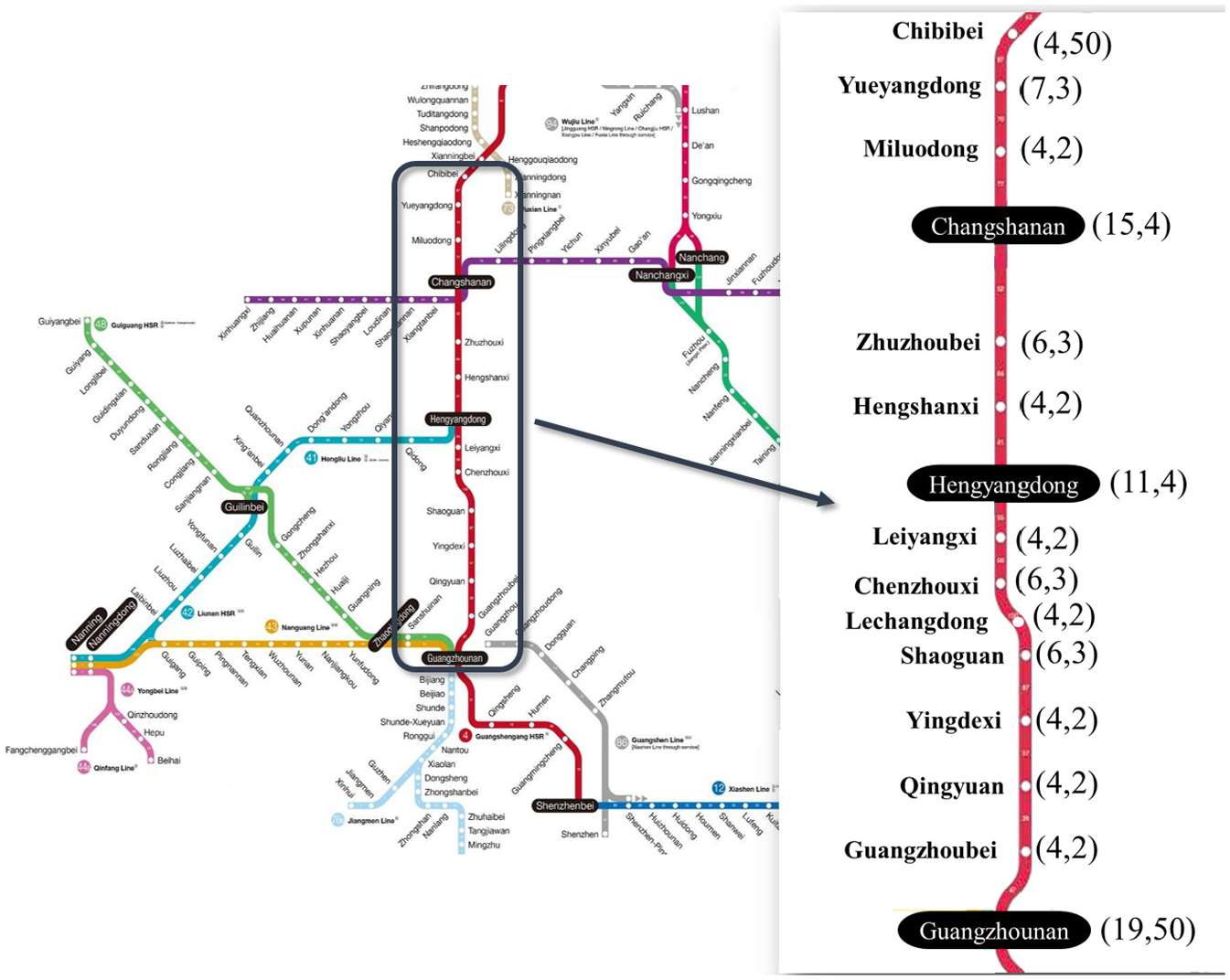
The Beijing–Guangzhou high-speed railway line from Chibibei to Guangzhounan.

The original timetable of the test line for July 2018, containing the data of 162 trains, is used. Three train route types are regarded as cross-line trains. As shown in Figure 6, black lines are local trains and blue lines are cross-line trains. There are 29 cross-line trains and 133 local trains in the original timetable.

Figure 6.

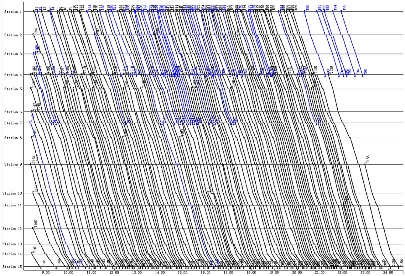
The original timetable used in experiments.

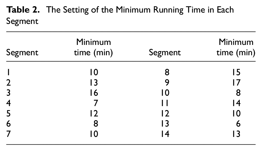
Through the statistics of the historical records, the minimum running time in each segment is obtained. Table 2 shows the minimum running time used in experiments. $L_{s_{i}}^{dwell}$ and $L^{dep, dep}$ are set as 2 min, while $L^{dep, arr}$ and $L^{arr, arr}$ are set as 3 min.

Table 2.

The Setting of the Minimum Running Time in Each Segment

Segment	Minimum time (min)	Segment	Minimum time (min)
1	10	8	15
2	13	9	17
3	16	10	8
4	7	11	14
5	12	12	10
6	8	13	6
7	10	14	13

Our experiments choose several disruption scenarios with different start times, durations, and locations. 9:00, 12:00, and 15:00 are chosen as the start time of the disruption. The locations are set as segments 5, 8, and 11. There are three values for duration, 30 min, 45 min, and 60 min. $M_{1}$ is set as 720 min and $M_{2}$ is set as 2000 min. The default values of penalty $γ_{cross}, γ_{local}, μ_{cross}, and μ_{local}$ are 100, 50, 2, and 1. Because we always get the exact end time of the disruption at its end, the default value of $ξ$ is set to 0.

Simulation Results and Discussion

In this section, we describe the simulation results obtained by applying the three-stage algorithm. For comparison, another MILP model is constructed directly using the original timetable and solved by CPLEX; this is called the one-stage algorithm in the next sections.

Results of Various Disruption Scenarios

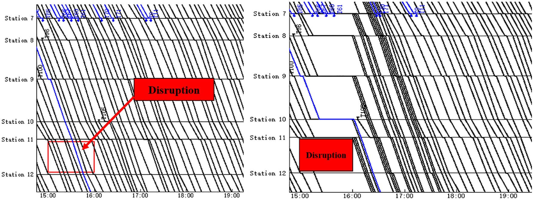
Figure 7 shows an example of the final timetable using the three-stage algorithm. In Figure 7, the blocked trains wait inside stations during the disruption. Since $ξ$ is equal to 0, trains can only depart from stations when the disruption ends.

Figure 7.

An example of the final timetable using the three-stage algorithm.

Table 3 shows the results for different instances, including the results of the one-stage algorithm. The instance $(a, b, c)$ means that the disruption occurs in segment $b$ , starting from time $a$ and lasting for time $c$ . The computational time limit of CPLEX is set to 900 s and the solving time of the three-stage algorithm is the total time of all three stages.

Table 3.

Results of Different Disruption Scenarios Using One-Stage or Three-Stage Algorithm

Instance	Objective with three-stage algorithm							Objective with one-stage algorithm
	Objective in Stage 1			Objective in final output				Objective with one-stage algorithm
	Value	Train number	Total delay	Value	Train number	Total delay	Solution time	Value	Solution time
(9, 5, 30)	1061	(1, 8)	(4, 553)	771	(0, 5)	(0, 521)	1	812	900
(9, 5, 45)	2489	(1, 9)	(5, 1929)	2311	(0, 9)	(0, 1861)	103	2278749	900
(9, 5, 60)	5792	(1, 16)	(49, 4794)	5078	(0, 12)	(0, 4478)	901	2575889	900
(9, 8, 30)	799	(1, 5)	(158, 133)	613	(1, 2)	(158, 97)	1	613	463
(9, 8, 45)	2093	(2, 8)	(371, 751)	1699	(1, 4)	(369, 661)	2	1699	564
(9, 8, 60)	3978	(1, 13)	(594, 2040)	3779	(1, 11)	(594, 1941)	54	2580207	900
(9, 11, 30)	743	(1, 6)	(6, 331)	551	(1, 3)	(6, 289)	2	551	462
(9, 11, 45)	1883	(2, 10)	(125, 933)	1400	(1, 6)	(6, 988)	5	2566156	900
(9, 11, 60)	3398	(1, 14)	(304, 1990)	3054	(1, 12)	(79, 2196)	65	2581001	900
(12, 5, 30)	1912	(3, 8)	(149, 914)	1441	(1, 6)	(154, 733)	9	1441	449
(12, 5, 45)	4901	(4, 15)	(347, 3057)	3733	(1, 12)	(244, 2545)	900	–	900
(12, 5, 60)	10080	(8, 17)	(836, 6758)	7350	(3, 15)	(423, 5454)	900	–	900
(12, 8, 30)	2317	(3, 10)	(441, 635)	1993	(2, 8)	(397, 599)	5	–	900
(12, 8, 45)	5411	(4, 16)	(908, 2395)	4524	(2, 13)	(831, 2012)	245	–	900
(12, 8, 60)	9599	(5, 20)	(1398, 5303)	8194	(2, 14)	(1281, 4732)	900	–	900
(12, 11, 30)	2596	(3, 14)	(318, 960)	2020	(1, 11)	(160, 1050)	134	2091	900
(12, 11, 45)	6303	(4, 22)	(755, 3293)	5273	(2, 18)	(517, 3139)	901	–	900
(12, 11, 60)	10601	(3, 21)	(1153, 6945)	9831	(2, 21)	(914, 6753)	901	–	900
(15, 5, 30)	3800	(8, 14)	(426, 1448)	2702	(4, 9)	(292, 1268)	900	2980	900
(15, 5, 45)	10479	(9, 17)	(1444, 5841)	7608	(9, 16)	(958, 3992)	901	8942	900
(15, 5, 60)	18840	(11, 21)	(2587, 11516)	15736	(11, 21)	(2138, 9310)	901	–	900
(15, 8, 30)	5141	(10, 12)	(1316, 909)	2606	(3, 8)	(704, 498)	60	2606	900
(15, 8, 45)	7247	(10, 17)	(1697, 2003)	5887	(6, 12)	(1482, 1723)	900	6145	900
(15, 8, 60)	15518	(11, 22)	(3361, 6596)	12230	(10, 19)	(2420, 5440)	901	–	900
(15, 11, 30)	4268	(10, 20)	(433, 1402)	2448	(3, 11)	(295, 1008)	148	2448	900
(15, 11, 45)	7970	(9, 24)	(1075, 3720)	6556	(6, 17)	(859, 3388)	901	6595	900
(15, 11, 60)	16536	(11, 29)	(2453, 9080)	12787	(8, 26)	(1943, 6801)	901	–	900

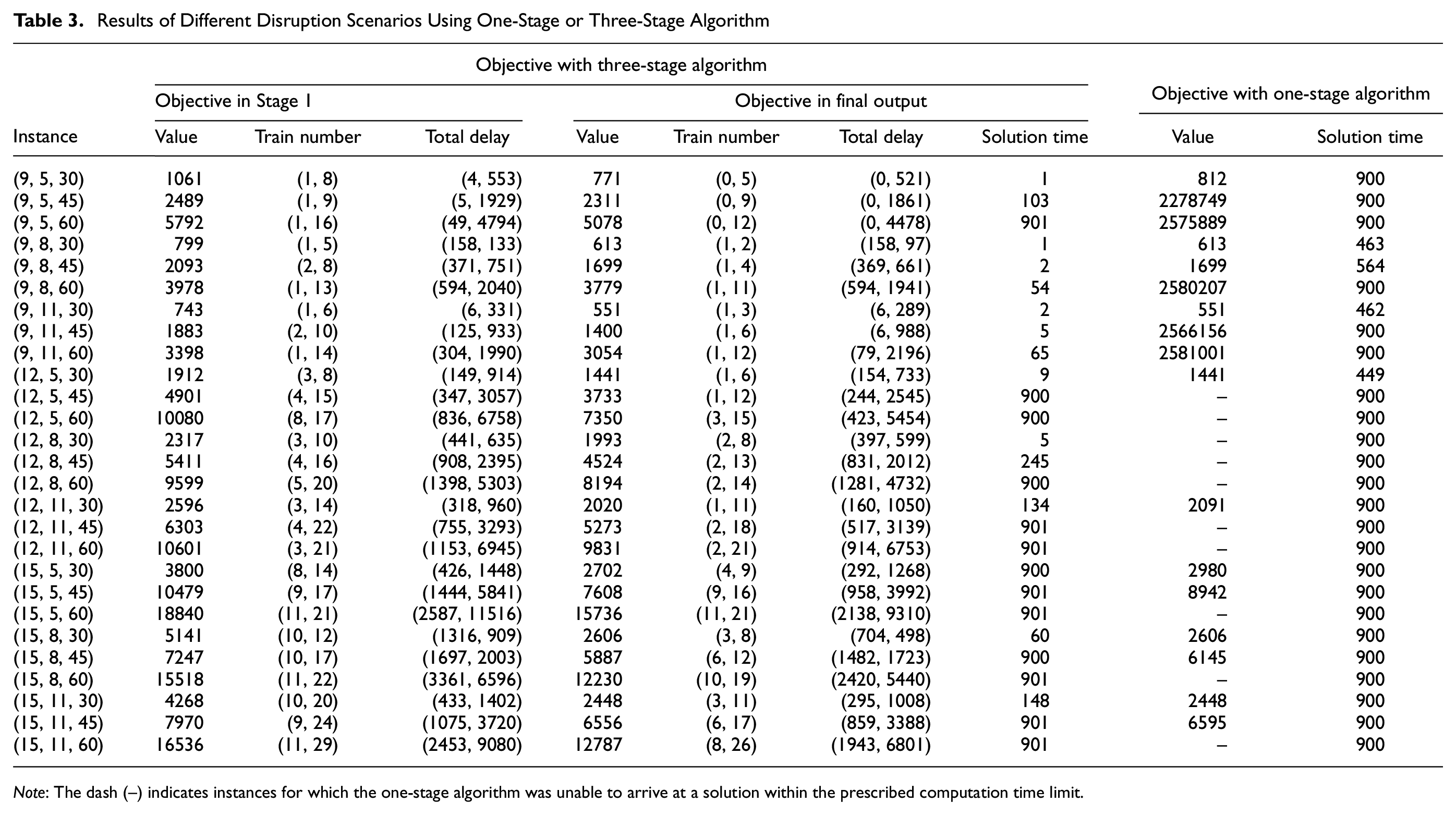
Note: The dash (–) indicates instances for which the one-stage algorithm was unable to arrive at a solution within the prescribed computation time limit.

Among these instances, there are 10 instances solved by the one-stage algorithm where no feasible result can be obtained within the limited computational time, which are marked as “–.” As the results shown in Table 3, our algorithm can produce optimized results under any circumstances, but in some cases one-stage algorithms cannot. Comparing the objective of the three-stage algorithm with the objective in Stage 1, these results indicate that the other two stages greatly optimize the feasible solution. A comparison of the data results using the two different algorithms shows that our algorithm can generate a superior objective value under the same time limit or generate the same optimal value with less solving time. This proves that the proposed algorithm performs well in the problem of timetable rescheduling and reduces the search space, which makes it easier to find good search results.

Computational Time Limits of CPLEX

To further illustrate the effectiveness of the three-stage algorithm, we choose instances with a solution time of up to 900 s and test them under different computational time limits. The computational time is limited to 150, 300, 450, 600, and 900 s. The results of Stage 1 are added to the graph for comparison. Figure 8 shows the results of these 13 instances.

Figure 8.

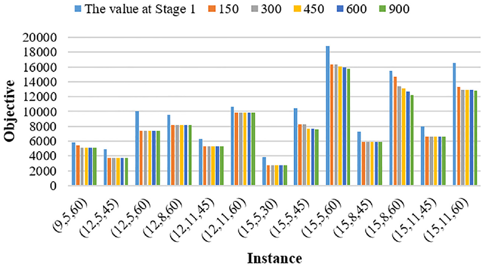
The objective of the three-stage algorithm under different computational time limits of CPLEX.

In Figure 8, we can see that all instances get a optimized objective in 150 s, which is much better than that at Stage 1. This fully proves the high efficiency of the remaining process of the three-stage algorithm. Moreover, except for the instances (15, 5, 60) and (15, 8, 60), most of the instances can achieve a better optimized solution within 450 to 600 s, and when the time limit increases, the objective value will not drop. In instances (15, 5, 60) and (15, 8, 60), the scale of the problem is too large to be solved in a short time, and the objective value will still slightly decrease as the time limit increases. This phenomenon is unavoidable in the face of large-scale problem solving. It is worth mentioning that our algorithm is an exhaustive search method. In fact, we will get a feasible result in each instance, which may be replaced soon by a better result over time. In these two instances, our three-stage algorithm can produce a feasible result within 150 s, while the one-stage algorithm cannot obtain a feasible solution within 900 s, which further proves that our method can solve large-scale problems well. To sum up, taking the scale of the problem into account, all instances using the three-stage algorithm can get a good solution within 450 to 600 s, which is acceptable for practical use.

The Building Time of the MILP Model

The solution time in Section 5.2.1 is without the building time of the MILP model. In this section we discuss the building time of different MILP models. We construct the MILP model using Python 3.7. Figure 9 shows the model building time when using different algorithms.

Figure 9.

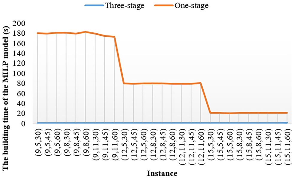
The building time of the mixed integer linear programming (MILP) model using different algorithms.

It can be seen from the experimental results that the building time of the one-stage algorithm is much longer than that of the three-stage algorithm. From the building time of the one-stage algorithm, we can find that the building time is inversely proportional to the start time of the disruption. The earlier the disruption occurs, the more trains are affected and the longer the building time is. This phenomenon shows that it is necessary to narrow the rescheduling range of trains. Since the average building time of 27 instances using the three-stage algorithm is 0.2 s, while that using the one-stage algorithm is 92.7 s, our algorithm can efficiently reduce the complexity of the problem.

Effect of Penalty Values

To evaluate the effect of penalties to the model solution, four value sets are selected for ( $γ_{cross}, γ_{local}, μ_{cross}, μ_{local}$ ). They are (100, 50, 2, 1), (2, 1, 100, 50), (10000, 50, 2, 1) and (2, 1, 10000, 50). The first and third sets give more weight to delayed train numbers, while the second and fourth sets give more weight to total delay time. More specifically, compared with the first set, the third set gives more weight to delayed cross-line train numbers. Compared with the second set, the third set gives more weight to delayed cross-line train numbers. Disruptions that start at 15:00 and last 30 min are taken as test instances. Table 4 shows the test results, where optimal results are marked as “^*” and the data ( $a, b, c, d$ ) for each cell refers to the target values corresponding to the penalties.

Table 4.

Final Results with Different Penalty Values

Instance	The result of stage	Penalty value
		(100, 50, 2, 1)		(2, 1, 100, 50)		(10000, 50, 2, 1)		(2, 1, 10000, 50)
		Value	Solution time	Value	Solution time	Value	Solution time	Value	Solution time
(15, 5, 30)	(8, 14, 426, 1448)	(4, 9, 292, 1268)	900	(6, 11, 326, 1142)^*	758	(2, 9, 263, 1867)^*	631	(2, 10, 235, 1985)	900
(15, 8, 30)	(10, 12, 1316, 909)	(3, 8, 704, 498)^*	60	(4, 8, 720, 460)^*	57	(3, 8, 704, 498)^*	46	(3, 8, 704, 498)^*	19
(15,11, 30)	(10, 20, 433, 1402)	(3, 11, 295, 1008)^*	148	(3, 11, 295, 1008)^*	146	(1, 11, 290, 1691)^*	841	(3, 12, 260, 1435)^*	128

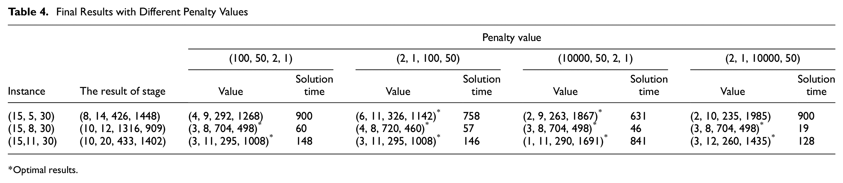
Optimal results.

From the statistics in Table 4, because these penalties change the search direction during the solution process, different penalty sets in each instance lead to different solution times. In theory, when the number of delayed trains and the total delay time are given different weights, the final result will also be different, just like the results of instance (15, 5, 30). In instance (15, 5, 30), when the delay time of the cross-line trains is given more weight, the final result will be less delay time of the cross-line trains, and more delay time of the local trains, and vice versa. However, the results of the first penalty set and the third penalty set in instance (15, 8, 30) are the same. This is because the number of delayed cross-line trains can no longer be reduced in the final result. Giving more weight to delayed cross-line trains will not change the optimal result. In addition, the results of the third penalty set and the fourth penalty set in instance (15, 8, 30) are the same too. It is because the optimal result has no room to reduce the number of trains and the weight change between local trains and cross-line trains in delay time is not enough to change the delay values. Moreover, the results of the first penalty set and the second penalty set in instance (15, 11, 30) are also the same. This is because neither the weight change in the train number between local trains and cross-line trains nor the weight change in the delay between local trains and cross-line trains is enough to change the final output. When the weight of the delayed number of cross-line trains or the weight of the delay time of cross-line trains continues to increase, such as the third penalty set and the fourth penalty set in instance (15, 11, 30), the final result can be changed. Therefore, it can be concluded that when there is room for adjustment in the final result, the higher the train number penalty, the fewer delayed trains; the higher the delay penalty, the less the delay. But to obtain the expected results, the appropriate weight should be carefully selected.

Function of Anticipation Abilities

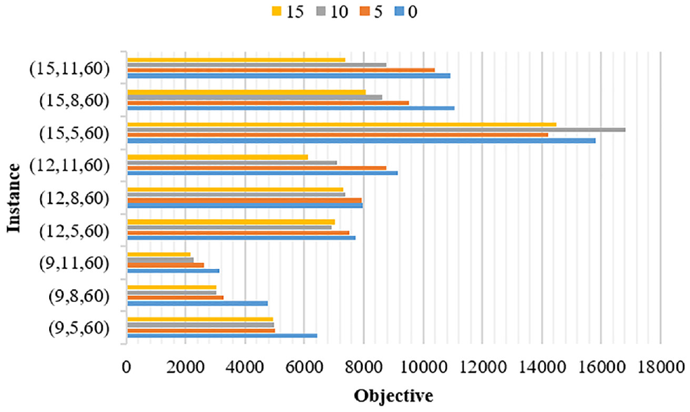
In the MILP model, the time when the blocked trains can depart from stations is related to the parameter $ξ$ of anticipation ability. To compare the difference between the models using different anticipation abilities, instances with a duration of 60 min are selected. Since the time that trains spend in segments cannot exceed the time in their original timetable, we test four values for parameter $ξ$ as 0, 5, 10, and 15 min. The computational time limit of CPLEX is set as 900 s. The results are shown in Figure 10.

Figure 10.

The objective in the final output using different anticipation abilities.

From Figure 10, it can be seen that in most cases, if the anticipation ability is greater, the objective value is better. Therefore, when facing with a large disruption, a great anticipation ability can help blocked trains quickly get back to normal. But there are exceptions. The results with the values of 15 min and 10 min in instance (15, 5, 60) are greater than that with the value of 5 min, and the result with the value of 15 min in instance (12, 5, 60) is greater than that with the value of 10 min. It is worth mentioning that all the results in these two instances are non-optimal solutions. So when enough solution time is given, the final result with a greater anticipation ability must be better. However, in a certain period of time, the greater the anticipation ability, the more choices for train selection, which increases the search space. In these instances, a better solution cannot be generated within 900 s.

Conclusions

In this paper, we developed a macroscopic real-time rescheduling approach for high-speed railway under a complete blockage. Aiming at minimizing the total delays and the number of delayed trains, a MILP model is proposed to generate a disposition timetable under the constraints of station capacities, activity time, overtaking rules, and rescheduling strategies. Our rescheduling strategy is that blocked trains must wait inside stations until the disruption ends, and when the exact end time of the disruption is known, trains at stations downstream of the blocked station can depart early. The model is applied on the part of Beijing–Guangzhou high-speed railway line from Chibibei to Guangzhounan with several disruption scenarios. There are in total 162 trains in the original timetable, combining 133 local trains and 29 cross-line trains. Since it is difficult to solve the MILP model directly in a short time, a three-stage algorithm is designed to accelerate the solution process.

Simulation results prove that our proposed method can handle the real-time timetable rescheduling problem under a case of complete blockage very well. Our approach has a higher solution efficiency and can meet different rescheduling requirements by changing penalties. Because all instances can obtain a better optimized disposition timetable within 450 to 600 s, our approach is acceptable for practical use. It is also found that a better anticipation ability can accelerate the recovery process, but may increase the search space, resulting in a failure to find a better solution within the specified time.

Several directions for further research are available. First, we find that the anticipation ability is very important for disruption recovery, which is not explored in this paper. Some research on the uncertainty of the disruption end time would be very meaningful if carried out to improve the anticipation ability. Second, we only consider the delays that occur on one line in this paper. However, in a railway network with cross-line trains, delays will spread to other lines as well. It is significant to build a method from the network level and study the strategy of using shared platforms for trains in different directions. Finally, trains that run from the same origin to the same terminus may have different routes to choose in a railway network. The measure of rerouting can be taken into account to solve the real-time rescheduling problem.

Footnotes

Acknowledgements

Thanks to our project partners for their useful contributions.

Author Contributions

The authors confirm contribution to the paper as follows: study conception and design: Bowen Gao, Decun Dong, Dongxiu Ou; data collection: Bowen Gao, Yusen Wu; analysis and interpretation of results: Bowen Gao, Yusen Wu; draft manuscript preparation: Bowen Gao, Yusen Wu, Dongxiu Ou. All authors reviewed the results and approved the final version of the manuscript.

Declaration of Conflicting Interests

The author(s) declared no potential conflicts of interest with respect to the research, authorship, and/or publication of this article.

Funding

The author(s) disclosed receipt of the following financial support for the research, authorship, and/or publication of this article: This research was supported by the Research Program of Comprehensive Support Technology for Railway Network Operation (No.2018YFB1201403), the Research Program of Shanghai Science and Technology Committee (No.18DZ2202600), and the National Natural Science Foundation of China (No.52172329).

ORCID iDs

Bowen Gao

Yusen Wu

References

Zhan

Kroon

L. G.

Veelenturf

L. P.

Wagenaar

J. C.

Real-Time High-Speed Train Rescheduling in Case of a Complete Blockage. Transportation Research Part B: Methodological, Vol. 78, 2015, pp. 182–201.

Cacchiani

Huisman

Kidd

Kroon

Toth

Veelenturf

Wagenaar

An Overview of Recovery Models and Algorithms for Real-Time Railway Rescheduling. Transportation Research Part B: Methodological, Vol. 63, 2014, pp. 15–37.

Corman

Lodewijks

A Review of Real Time Railway Traffic Management during Disturbances. In Computational Logistics. ICCL 2015. Lecture Notes in Computer Science ( Corman

Voß

Negenborn

, eds.), Springer, Cham, Vol. 9335, 2015, pp. 658–672.

Ghaemi

Cats

Goverde

R. M.

Railway Disruption Management Challenges and Possible Solution Directions. Public Transport, Vol. 9, No. 1–2, 2017, pp. 343–364.

Corman

D’Ariano

Hansen

I. A.

Pacciarelli

Optimal Multi-Class Rescheduling of Railway Traffic. Journal of Rail Transport Planning & Management, Vol. 1, No. 1, 2011, pp. 14–24.

Corman

D’Ariano

Pacciarelli

Pranzo

Bi-Objective Conflict Detection and Resolution in Railway Traffic Management. Transportation Research Part C: Emerging Technologies, Vol. 20, No. 1, 2012, pp. 79–94.

Caimi

Fuchsberger

Laumanns

Lüthi

A Model Predictive Control Approach for Discrete-Time Rescheduling in Complex Central Railway Station Areas. Computers & Operations Research, Vol. 39, No. 11, 2012, pp. 2578–2593.

Chu

Oetting

Modeling Capacity Consumption Considering Disruption Program Characteristics and the Transition Phase to Steady Operations during Disruptions. Journal of Rail Transport Planning & Management, Vol. 3, No. 3, 2013, pp. 54–67.

Pellegrini

Marlière

Rodriguez

Optimal Train Routing and Scheduling for Managing Traffic Perturbations in Complex Junctions. Transportation Research Part B: Methodological, Vol. 59, 2014, pp. 58–80.

10.

Ghaemi

Cats

Goverde

R. M.

A Microscopic Model for Optimal Train Short-Turnings during Complete Blockages. Transportation Research Part B: Methodological, Vol. 105, 2017, pp. 423–437.

11.

Veelenturf

L. P.

Kidd

M. P.

Cacchiani

Kroon

L. G.

Toth

A Railway Timetable Rescheduling Approach for Handling Large-Scale Disruptions. Transportation Science, Vol. 50, No. 3, 2016, pp. 841–862.

12.

Meng

Zhou

Robust Single-Track Train Dispatching Model under a Dynamic and Stochastic Environment: A Scenario-Based Rolling Horizon Solution Approach. Transportation Research Part B: Methodological, Vol. 45, No. 7, 2011, pp. 1080–1102.

13.

Louwerse

Huisman

Adjusting a Railway Timetable in Case of Partial or Complete Blockades. European Journal of Operational Research, Vol. 235, No. 3, 2014, pp. 583–593.

14.

Zhan

Kroon

L. G.

Zhao

Peng

A Rolling Horizon Approach to the High Speed Train Rescheduling Problem in Case of a Partial Segment Blockage. Transportation Research Part E: Logistics and Transportation Review, Vol. 95, 2016, pp. 32–61.

15.

Binder

Maknoon

Bierlaire

The Multi-Objective Railway Timetable Rescheduling Problem. Transportation Research Part C: Emerging Technologies, Vol. 78, 2017, pp. 78–94.

16.

Ghaemi

Cats

Goverde

R. M.

Macroscopic Multiple-Station Short-Turning Model in Case of Complete Railway Blockages. Transportation Research Part C: Emerging Technologies, Vol. 89, 2018, pp. 113–132.

17.

Zhu

Goverde

Railway Timetable Rescheduling with Flexible Stopping and Flexible Short-Turning During Disruptions. Transportation Research Part B: Methodological, Vol. 123, No. 5, 2019, pp. 149–181.