
Abstract
Aggregation of sparse probe vehicle data (PVD) is a crucial issue in travel time reliability (TTR) analysis. This study, therefore, examines the effect of temporal and spatial aggregation of sparse PVD on the results of a linear regression analysis where two different measures of TTR are analyzed as the dependent variable. Our results show that by aggregating the data to longer time intervals and coarser spatial units the linear model can explain a higher proportion of the variance in TTR. Furthermore, we find that the effects of road design characteristics in particular depend on the variable used to represent TTR. We conclude that the temporal and spatial aggregation of sparse PVD affects the results of linear regression explaining TTR.
Keywords
The analysis of travel time reliability (TTR) is of high interest for traffic planners and road authorities. The New Zealand Transport Agency ( 1 ) defines TTR as the reliability of travel times that occur for a journey made at approximately the same time each day. To explain this phenomenon, it is necessary for researchers to define the levels of spatial and temporal aggregation of the data on which the evaluation of TTR is based. Especially in the case of sparse probe vehicle data (PVD), temporal and spatial aggregation are crucial issues in analyzing the roots of TTR. PVD can be aggregated based on temporal (the width of time-of-day [TOD] intervals) and spatial (the length of road segments) characteristics. A temporal and spatial aggregation that is too narrow makes the results vulnerable to outliers, while too broad a definition can lead to information loss. There is a large literature explaining TTR which includes the effect of geometrical characteristics ( 2 – 4 ), lane choice of the drivers ( 5 ), capacity factors ( 5 ), weather situations ( 3 , 4 , 6 , 7 ), incidents ( 3 , 4 , 6 , 8 ), and traffic demand ( 4 ) on TTR. However, to the best of our knowledge, current research neglects the question of how to adjust the temporal and spatial aggregation of sparse PVD in explaining TTR. This paper, therefore, aims to fill this gap and by providing a methodology to analyze the effect of different temporal and spatial aggregations of sparse PVD. For this purpose, we apply a linear regression model to explain the travel time index (TTI) and the standard deviation (SD) as two examples of TTR measures.
In this context we want to answer the following research question: How does the temporal and spatial aggregation of sparse PVD affect the results of a linear regression analysis when it comes to explaining the factors influencing TTR?
To answer this question, we propose a methodology to evaluate temporal and spatial settings of aggregating sparse PVD on explaining TTR. Thus, a regression approach will be used to investigate which variables have a significant influence on TTR. Interval lengths of 15, 30, and 60 min are used as temporal modeling of PVD, while two variants of spatial segmentation in the form of links and sections are used for spatial modeling. The data analyzed are a raw data set without interpolation of missing values. Since most researchers work with an interpolated data set, the results of this study are particularly interesting for raw data providers or researchers who have non-interpolated data sets. The evaluation is divided into two parts. First, we run a linear regression for each model variant and check whether or how the influence of the independent variables (IVs) changes with respect to different spatial and temporal aggregation levels of the data used. In this context, we also check how much of the variation in the dependent variable (DV) can be explained by the IVs and how this differs between the models. In a second step, we analyze the predictive performance of the models calibrated in the first step by applying them to a test data set to predict TTR. We then calculate the root mean square error (RMSE) and the mean absolute percentage error (MAPE) between the predicted and the observed TTR measure for each model variant. Moreover, we provide analysis of whether our models fulfill the general assumptions of linear regression models. In addition, we perform a robustness check to see if the evaluation results change when using a different time period.
Literature
Our research question demands a review of two strands of literature. First, we analyze how TTR is explained and what kind of characteristics are used to explain TTR. Second, we analyze how the effects of different levels of temporal and spatial aggregation of travel time data are measured.
The Explanation of TTR
Tu et al. ( 2 ) analyze the impact of geometrical characteristics of freeways on TTR, such as the number of ramps or the length of acceleration lanes. Their results provide traffic planners with threshold values for the analyzed geometric features to achieve a lower TTR. Li et al. ( 9 ) use automatic vehicle identification (AVI) data and apply multiple regression to show the components of TTR. Their results illustrate that the TTR during the morning peak is most influenced by the lane choice of the drivers, while during the afternoon peak TTR is most influenced by capacity related factors. Tu et al. ( 5 ) analyze the relationship between inflow levels for road capacity and TTR on highway corridors. As a result, the authors show critical inflow levels that affect TTR. Higatani et al. ( 10 ) empirically analyze the characteristics of various TTR indices for the Hanshin expressway network. Their main result shows that the buffer time and the buffer time index behave similarly to the SD and the coefficient of variation, respectively. Martchouk et al. ( 6 ) use anonymous Bluetooth-collected freeway travel time data from Indianapolis to analyze the TTR. The authors show that adverse weather situations, unexpected changes in traffic flow, and driver behavior have a significant impact on TTR. Known et al. ( 4 ) decompose the buffer time into five components which could be divided into three groups: traffic influencing events (incidents, work zone activity and weather), traffic demand (special events), and physical highway features (bottlenecks). The authors find that recurring bottlenecks contribute most to the buffer time, while traffic accidents are the second largest driver with 15.1% contributing to TTR during the morning and 25.5% during the afternoon. Yazici et al. ( 11 ) analyze the differences in TTR patterns between urban roads and highways. They use GPS taxi data and automatic vehicle location data to calculate the SD and the coefficient of variation. Furthermore, they visually compare the travel time distribution for different time slots among facility types. Their main result shows that on freeways higher travel times are positively correlated with the coefficient of variation, whereas on urban roads they are negatively correlated. Yang et al. ( 12 ) measure TTR by first estimating travel time distributions using kernel density estimations. In a next step they use the Hasofer-Lind-Rackwitz-Fiessler algorithm to compute a TTR index for corridors and networks respectively that measures on-time performance. Hojati et al. ( 8 ) analyze the effects of non-recurrent events on TTR. The authors use a Tobit Regression to understand what affects the buffer time index. Their results show that the incident details and the traffic related characteristics are important to explain the negative impacts on the TTR with regard to traffic incidents. Javid and Javid ( 3 ) provide a framework to estimate the effect of traffic incidents on TTR. The authors use integrated traffic, road geometry, incident, and weather data for a two-year period from highways in California and apply a set of robust regression models. Their results show an adverse impact of highway shoulder and lane width on downstream highway clearance time. In addition, Javid and Javid ( 3 ) show that in the event of traffic accidents at weekends, highway clearance is shorter. Chen et al. ( 13 ) analyze TTR patterns for Beijing using PVD. Their results illustrate that for weekdays, morning and afternoon peaks vary among road types. Interestingly, the variability measures used are not consistent in their conclusions as the buffer time index remains constant while the COV shows varying results. Chen and Fan ( 7 ) use a data-driven approach to analyze patterns in TTR. They apply a time series model with PVD from freeway segments to predict the planning time index. Their results show that the planning time index is lower on weekends and higher under rain and snow conditions. Siddiqui and Ko ( 14 ) use a generalized linear model to explain the following three measures: TTR, freight TTR, and traffic congestion. The authors find that directional annual average daily traffic and urban areas are the two features with the highest positive association for these three measures. On the other hand, they find that the number of through lines are the feature which is most negatively associated. Interestingly, the length of a segment shows no clear results among the three measures.
The Impact of the Temporal and Spatial Aggregation of Travel Time Data on TTR
Mori et al. ( 15 ) argue that aggregation and simplification of travel time data are used to reduce the cost of storage and calculation, which could lead to loss of information if not done properly. Zietsman and Rilett ( 16 ) use data from AVI to analyze the effect of temporal and spatial disaggregation on the accuracy of travel time and travel time variability estimation. The authors apply the MAPE and linear regression to find the most appropriate level of aggregation. As a temporal aggregation, the authors use an aggregation across days and by days. With respect to spatial aggregation, they estimate performance measures with link-based and corridor-based techniques. The authors argue that corridor travel times show a similar accuracy when calculated with link travel times. Furthermore, their results show the uniqueness of individual travel patterns and the benefits when performance measures are analyzed at the individual commuter level. The authors conclude that data disaggregation should be preferred to an aggregated approach when estimating travel time and TTR. Wang and Liu ( 17 ) analyze traffic delays in relation to various characteristics of loop detector data, including loop detector distance (31, 183, 305, and 610 m) and data aggregation intervals (30, 60, and 300 s). The authors use the difference between loop detector-estimated and ground truth travel time delay and calculate the Mean Absolute Error and the MAPE. Their results show that shorter loop detector distances and longer data aggregation intervals lead to better estimation results. Oh et al. ( 18 ) analyze the relationship between temporal aggregation of traffic data and travel time prediction. The authors, therefore, used an inductive signature-based vehicle reidentification system to collect traffic data on a freeway. They compared aggregation intervals ranging from 1 to 10 min and applied adaptive exponential smoothing, an autoregressive model, and a recurrent neural network to predict travel times. Their results show that an aggregation interval of 4 to 6 min is best suited for their data set, as is able to capture traffic dynamics and show sufficient accuracy. Park et al. ( 19 ) present a methodology to identify the optimal aggregation interval sizes for estimating and forecasting travel times. Their evaluation metric consists of comparing single travel times to the sample mean and comparing the sample mean to the true mean, which needs to be estimated first. The authors apply this methodology to data from an AVI system during the morning peak. Their results show that the optimal aggregation interval depends on the application and traffic conditions. Interestingly, for estimating route travel times aggregation intervals should be higher than for estimating link travel times. Bigazzi et al. ( 20 ) investigate the impact of temporal aggregation on performance measures and Intelligent Transportation Systems applications. The authors use data from freeways by using inductive dual-loop detectors and a video image detection system. Their results show that data aggregation reduces the spread of speed measures and therefore distorts the results of travel estimation. Finally, the authors mention that temporal aggregation has implications for identifying traffic state transition times, estimating shock wave propagation times, and fundamental diagrams.
The review shows that the literature focuses on the impact of travel time aggregation on TTR accuracy, travel time prediction, and performance measures. However, the data used in these studies comes from stationary data acquisition systems with high penetration rates compared with PVD.
The analysis of the literature explaining TTR shows a wide range of explanatory variables. However, none of these studies analyzes the impact of temporal and spatial aggregation of the data used in the analysis. On the other hand, the analysis of the literature on the effect of temporal and spatial aggregation of travel time data on TTR or travel time shows that these studies use data with relatively high penetration rates compared with PVD. Our aim is, therefore, to fill this gap and analyze how the results of a linear regression change when different aggregated data sets of PVD are used. First, we want to show whether or how the influence of IVs on TTR changes between spatially and temporally different data aggregation settings of sparse PVD. We also want to show how the proportion of the variance of the DV explained by the IVs changes between spatially and temporally differently aggregated sparse PVD. Furthermore, we want to show how the predictive power of linear regressions changes when different temporal and spatial levels of aggregated sparse PVD are used.
Methodology
Spatial and Temporal Aggregation
To define the spatial and temporal aggregation levels, we follow an approach by Steinmaßl et al. ( 21 ). We analyze our results depending on the TOD in 15-, 30-, and 60-min intervals. We assume that the results vary greatly between these three intervals. According to Steinmaßl et al. ( 21 ), a coarser level of temporal aggregation means that significant short-term variations of travel times could not be detected, as they might be lost in the aggregation. Thus, the effect of road construction elements or peak hour could not be identified. On the other hand, temporal aggregation that is too fine may lead to inaccurate TTR values, as the calculation could depend on a very small number of observations when PVD is sparse.
For the spatial aggregation, we use two different segmentations that vary in length depending on the ontology of the map. For the definition of these two types, we adopt the approach of Steinmaßl et al. (
21
) and define a spatial unit as a road segment between two turn options. The turn options of a road network representation depend on its level of detail. Following Steinmaßl et al. (
21
), we use two different network representations based on the Functional Road Classes (FRCs) of roads. In our case, FRCs are defined by the Austrian Graph Integration Platform (GIP.AT) and classify roads hierarchically according to their importance from a traffic planning and network logic perspective. The FRC is represented by ascending integers starting with a value of
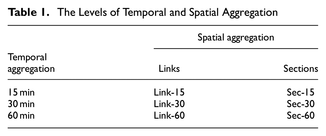
For the calculation of the TTR of a link or a section, the travel times of those vehicles that have completely passed through it in a respective TOD interval are taken into account. With the three temporal and two spatial aggregations, we have six ways in which TTR is calculated from PVD. These six ways are shown in Table 1 and form the levels of aggregation, which we use for the analysis.
The Levels of Temporal and Spatial Aggregation
Measuring Traffic Time and its Reliability
In principle, TTR can be defined as the reliability of travel times ( 11 ). A more detailed definition explains TTR as variations in travel time that occur for trips made at the same time every day ( 1 ). The TTI reflects this definition as it represents the delay in travel time compared with travel time under free flow conditions. In addition, the TTI is a standardized measurement and is therefore suitable for comparing links/sections with different lengths. Thus, we decided to use the TTI as one measure to analyze TTR. The TTI is defined as follows:

where
The free flow travel time can be defined as the travel time under free flow conditions ( 22 ), occurring at the 85th percentile of velocities ( 7 , 23 ).
However, in this study we also apply an additional approach and measure TTR as the variation of travel time in predefined TOD intervals on a daily basis. Therefore, we choose the SD, a common metric for measuring TTR ( 24 ), which represents the distribution of travel times with the following formula:

where
In conclusion, we measure TTR with two different concepts. First, the TTI represents a TTR measure that is defined as a normalized average travel time at the respective TOD. Secondly, SD represents TTR as the variation of travel times in a given TOD interval on a given day, independent of travel times measured on other days in that given TOD interval.
Data
For the evaluation, we use sparse PVD from the Austrian National Floating Car Data Platform (
25
). The PVD result from signals of the Global Navigation Satellite System (GNSS), which make it possible to calculate a time-referenced position of a vehicle. To map these positions, we use an algorithm by Rehrl et al. (
26
), which is based on the work of Sauerwein (
27
). The evaluation network used for this study is shown in Figure 1 and consists of nine entry routes into the city of Salzburg. In total, the analyzed routes consist of
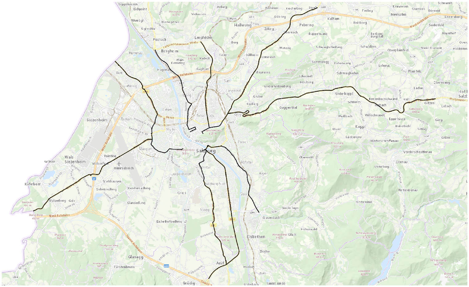
Overview of routes.
For the evaluation, we use a data set ranging from June 3 to August 4, 2019. We split this data set into training and testing data sets. The training data set ranges from June 3 to July 14, while the test data set ranges from the July 15 to August 4. The majority of the findings in this paper are based on the training data set. The test data set is only used when the predictive performance of the linear regression model is tested. To ensure comparability of our data with future studies, we calculate three indices representing the sparseness of our data set.
Figure 2 illustrates the proportion of at least one observation per link/section and TOD interval for each temporal aggregation respectively. This means that Figure 2 shows the percentage of links and sections where data from at least one vehicle was recorded. We find that at the 15-min interval, this value ranges from around
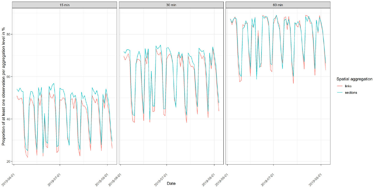
Proportion of at least one observation per aggregation level.
Figure 3 illustrates the mean number of observations per aggregation level. It can be seen that the values in the 15-min interval range from about
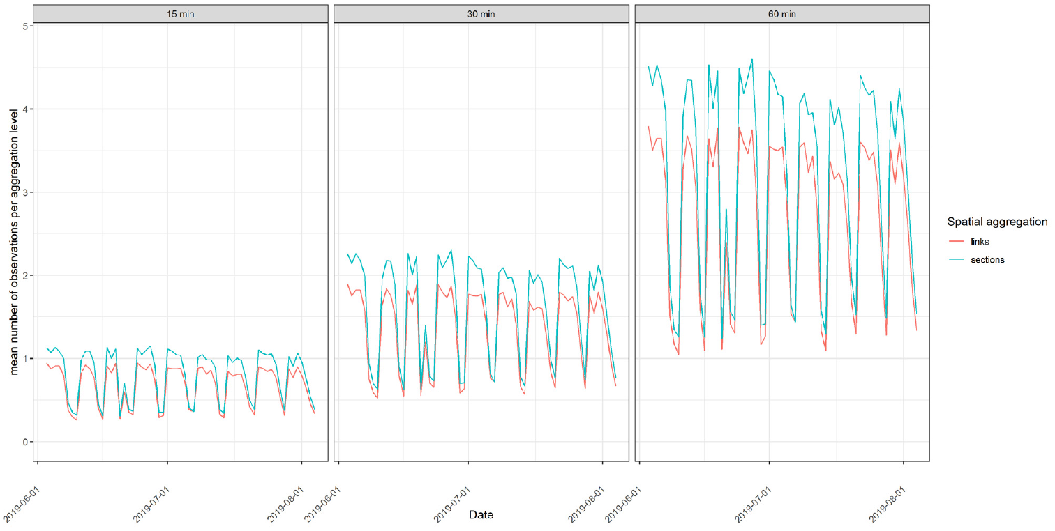
Mean number of observations per aggregation level.
Figure 4 shows the absolute number of observations per day. We find that the absolute number of observations for links ranges from about
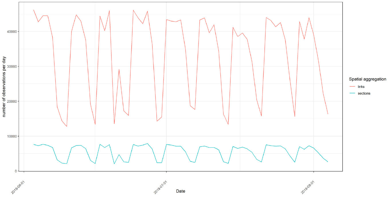
Absolute number of observations per aggregation level.
To remove outliers from the data set, we decided to filter extreme values depending on the DV. To determine the thresholds for outlier filtering, we conducted an empirical analysis. We, therefore, use histograms that allow us to analyze the distribution of our DV and identify outliers at the respective left and right ends. Table 2 shows the lower and upper bounds for the respective aggregation level. When we use SD as DV, the lowest and the highest
Lower and Upper Bounds of the Dependent Variables of the Respective Temporal and Spatial Aggregation of the Data
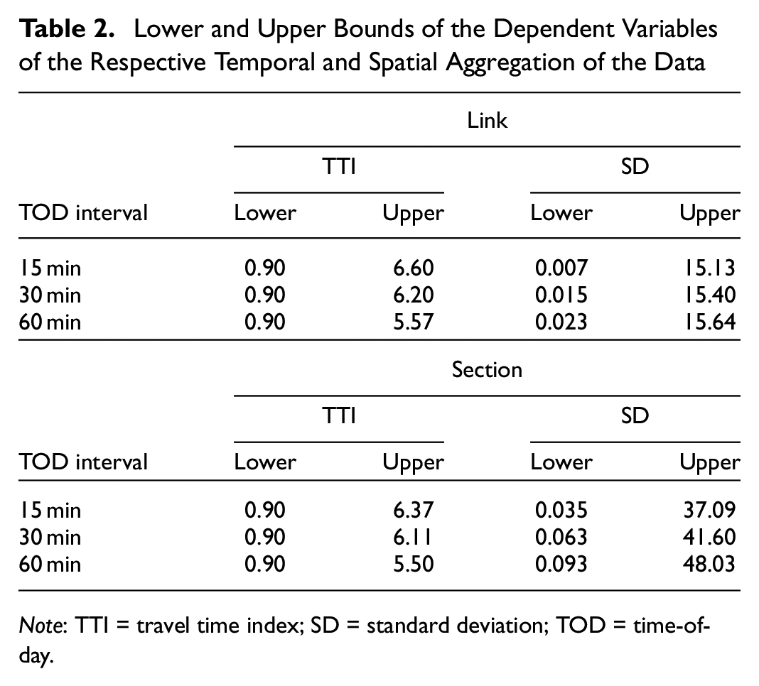
Note: TTI = travel time index; SD = standard deviation; TOD = time-of-day.
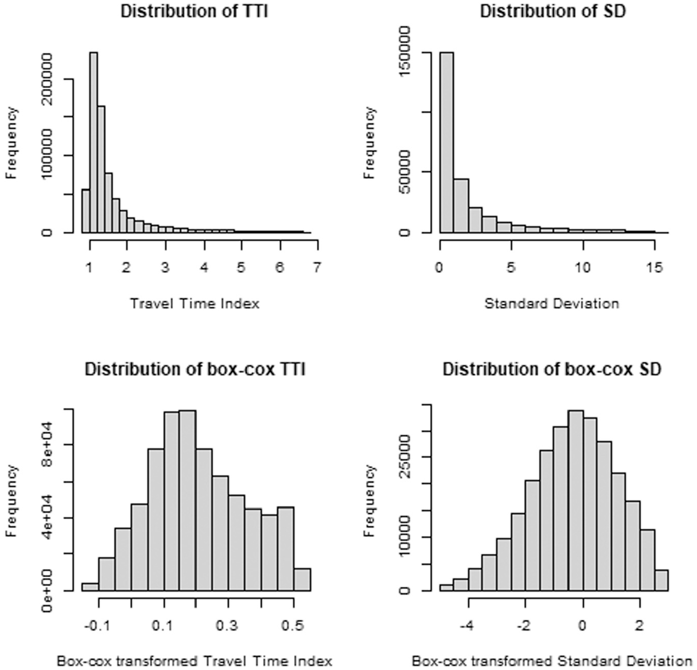
Distribution of Dependent Variables, Link-15.
Analysis
To assess the proportion of the variance of the DV explained by the IVs and whether or how the influence of IVs on TTI and SD changes with respect to different temporal and spatial aggregation levels of data, we apply the linear regression model in Equation 3. Therefore, we use
Dependent Variables (DV) and Independent Variables (IV) of the Linear Regression Model
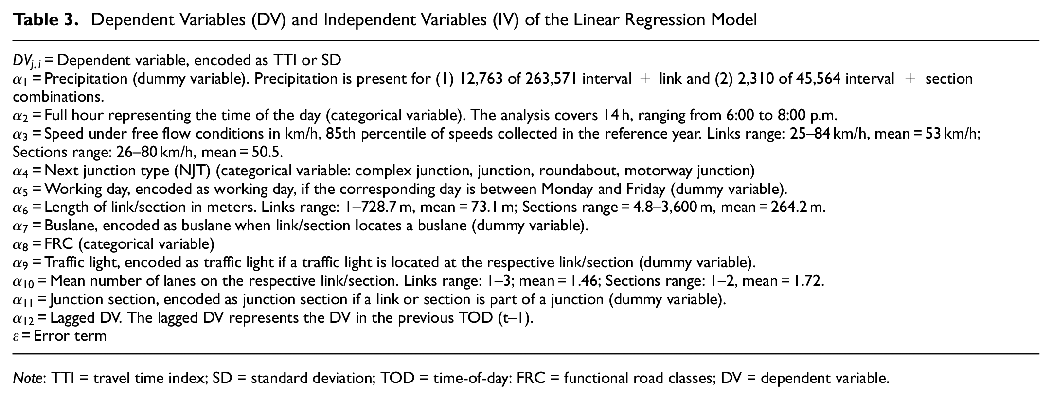
Note: TTI = travel time index; SD = standard deviation; TOD = time-of-day: FRC = functional road classes; DV = dependent variable.
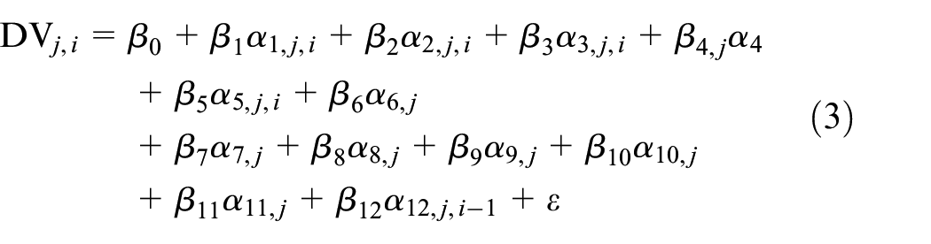
where
Some of these variables need a more detailed explanation that we provide below. Since the relationship between TOD and traffic is nonlinear, we encode TOD as a categorical variable. Independent of the temporal aggregation of the data, we use the corresponding full hour of a TOD interval to assure comparability between differently aggregated data. The free flow speed is included to model a possible dependency on the general speed level of a link or section. To classify junctions we follow an approach based on Rehrl et al. (
29
). The variable “next junction type” refers to junctions within the higher-level road network only. Junctions on a lower-level road network (FRC
We also considered including a variable “form of way” to describe constructional properties of links or sections, for example, if lanes of different direction are divided by barriers. However, because of multicollinearity, we excluded it from the final model which will be discussed in the results section.
We have to mention that the inclusion of additional explanatory variables could be helpful to explain the TTR. In this context, we think of information on the general state of traffic, such as total traffic volume. In addition, information on incidents can improve the performance of the models. While we do not have information on total traffic volumes, we do have data on accidents, which is too spatially coarse to be included in the analysis.
For the evaluation we apply two steps. In a first step, we train the linear model using the training data set. We then analyze the regression results and show whether or how the effects of the IVs vary when using different temporal and spatial aggregation levels of the data. We also analyze how the adjusted
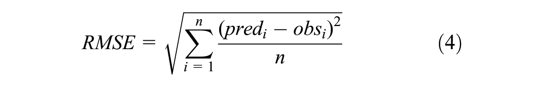

where
To interpret the results of the MAPE we follow the categorization framework of Lewis ( 30 ) in Table 4.
Forecasting Power
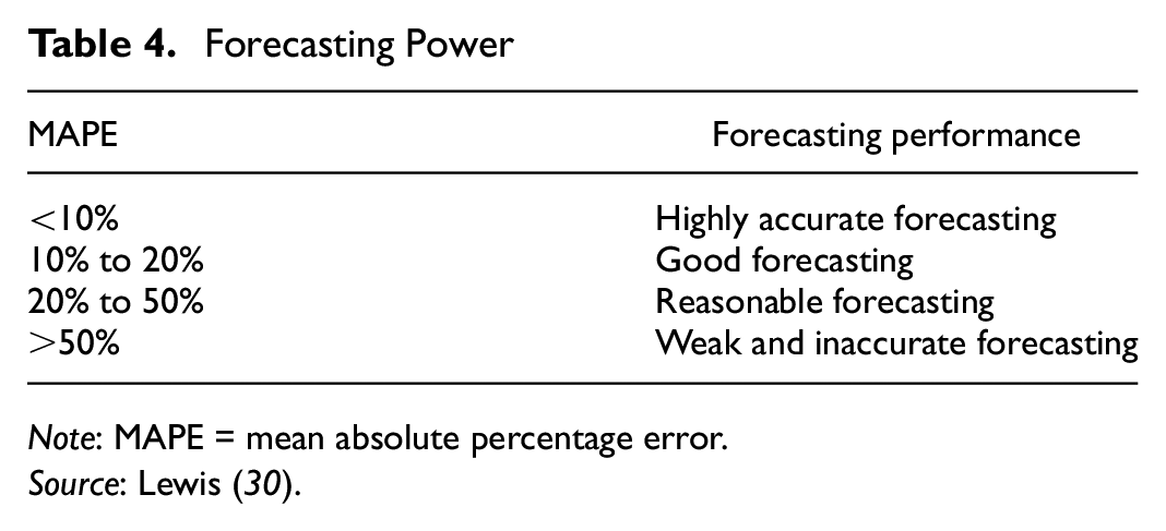
Note: MAPE = mean absolute percentage error.
Source: Lewis ( 30 ).
Evaluation
Model Diagnostic
Before we start with the evaluation, we would like to mention that all results presented in this paper were calculated with the statistical software R ( 31 ). Moreover, we use the following packages for the analysis: ggplot2 ( 32 ), stargazer ( 33 ), and dplyr ( 34 ).
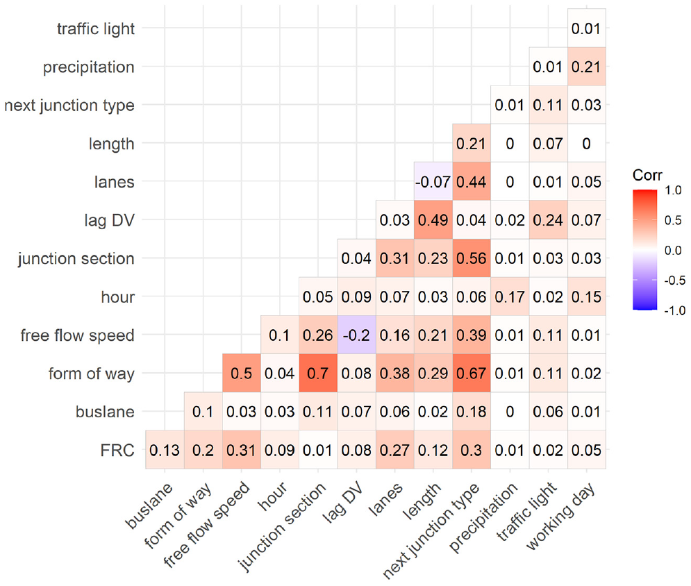
To check whether the linear regression model works well for our data, we control for various statistical assumptions and present detailed model diagnostics. For reasons of readability, we only give a detailed analysis of the model diagnosis for the aggregation level Link-15 for TTI or SD as DV. However, this calibration represents the worst model diagnostics, as we find better results when using longer TOD intervals and sections instead of links as spatial aggregation. First, we test for multicollinearity in our data. Figures 6 and 7 show association matrices and illustrate how the IVs are correlated with each other. To calculate associations between IVs, we use the following approaches for the respective variable combinations: Pearson correlation (numeric versus numeric), a bias corrected Cramer’s V (categorical versus categorical), and ANOVA (categorical versus numeric). The results show that the IV form of way seems to be highly correlated with the IVs next junction type and junction section. Therefore, we decided to not consider the IV form of way in the final model.
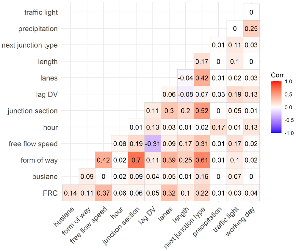
Assosiaction matrix, Link-15, TTI.
Assosiaction matrix, Link-15, standard deviation.
Figures 8 and 9 present additional model diagnostics when using the aggregation level Link-15 with TTI or SD as the DV. The plot at the top left illustrates the residuals versus fitted plot and indicates whether we can assume linearity in the data. As the red line moves around the horizontal line and shows no specific pattern, we would assume a linear relationship between the DV and the IVs. The plot at the top right shows the quantile–quantile plot and indicates whether the residuals are normally distributed. To confirm this assumption the residuals should follow the dotted line, which is approximately the case in our example. At the bottom left we find the scale-location plot, which allows us to check the presence of homoscedasticity. In the case of homoscedasticity the red line should be horizontal as this would imply that the residuals show constant variances. According to the results in the plots we can assume homoscedasticity for both DVs. We also use the Breusch-Pagan test to support the visual analysis of homoskedasticity. However, according to the results of the Breusch–Pagan test, we cannot assume homoscedasticity for our model. Given the large sample size, it is likely that the explanatory variables explain some of the variance in the residuals. Consequently, the model lacks some explanatory information, which remains in the residuals. However, since the visual analysis does not support the assumption of a strong degree of homoscedasticity, we do not assume strong effects for our model.
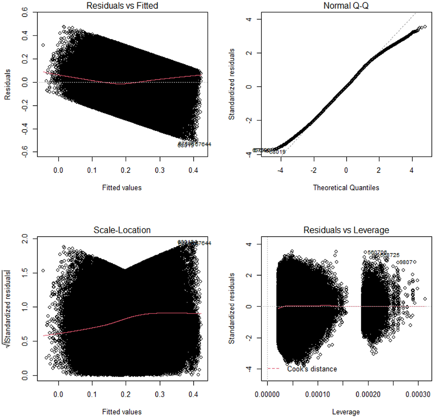
Model diagnostic, Link-15, travel time index (TTI).
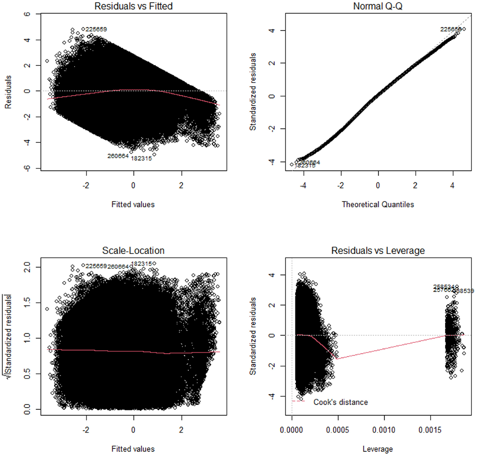
Model diagnostic, Link-15, standard deviation (SD).
Finally, the plot at the bottom right shows if any outliers heavily influence the model output. We would consider it a problem if one of the points lay outside the area that is marked with Cook’s Distance. As this is not the case, we would assume no outliers that heavily influence our models outcome.
We also check whether our model suffers from autocorrelation and test whether two consecutive residuals from our model have a non-zero correlation. To do this, we apply a Durbin–Watson test ( 35 , 36 ). Table 5 shows that using linear regression as described in Equation 3 without a lagged DV, the model suffers from autocorrelation for all levels of temporal or spatial aggregation of the data. However, after including a lagged DV as an IV, the DW test shows a p-value of 1, indicating that the model has no autocorrelation. This is plausible because the TTR between two consecutive intervals is usually similar and therefore correlates with the TTR of the previous interval.
Durbin-Watson Statistics With and Without Lagged DV
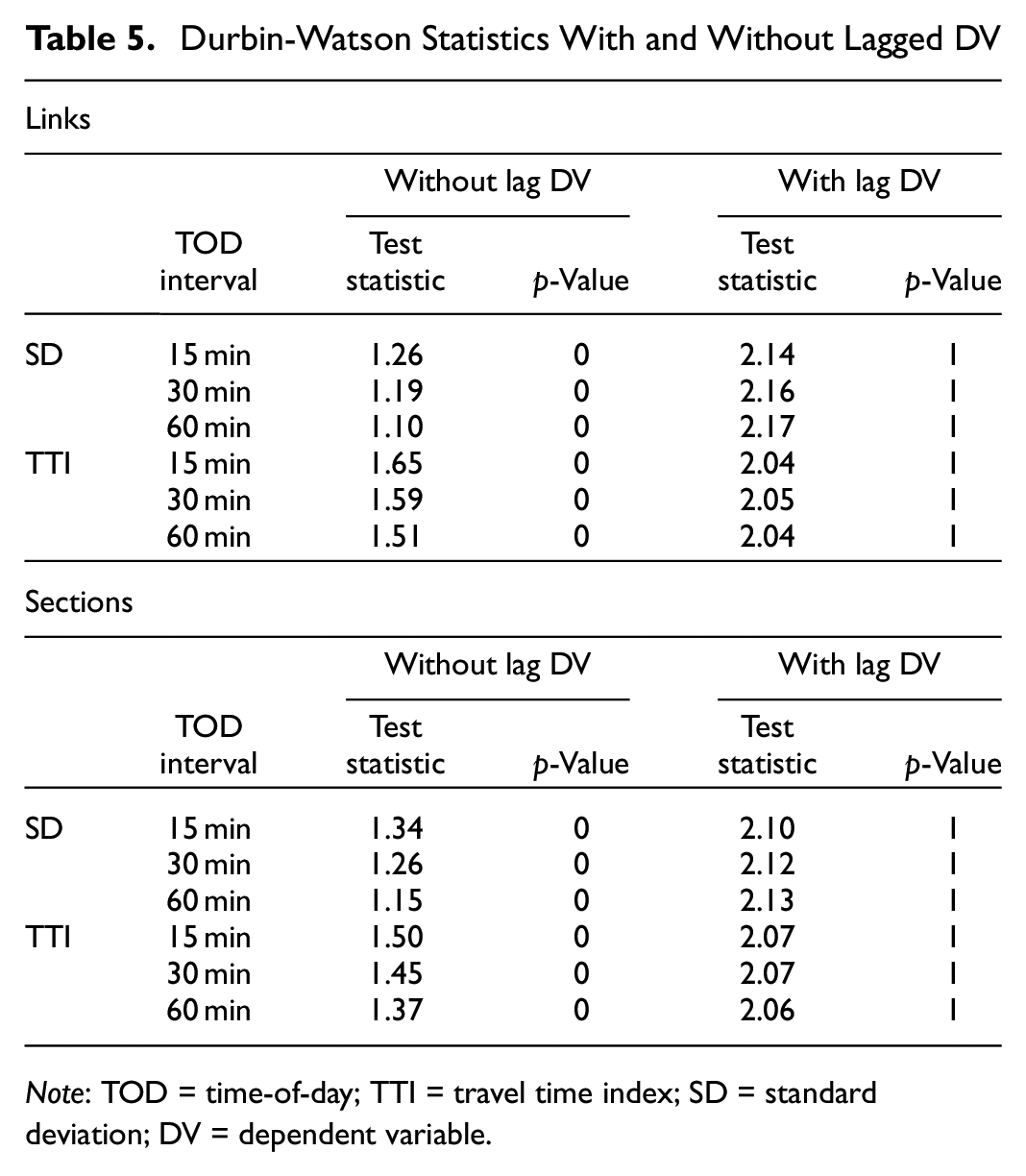
Note: TOD = time-of-day; TTI = travel time index; SD = standard deviation; DV = dependent variable.
Thus, we find that, according to the results of the model diagnostics, there is a linear relationship between the DV and the IVs, the residuals are normally distributed and there are no extreme values with high influence on the model results. However, we do not find clear results with respect to the assumption of homoscedasticity, as the visual analysis would lead to the conclusion that homogeneity of variance of the residuals prevails, but the Breusch–Pagan test indicates the opposite. We must therefore assume that some information of the model remains in the residuals. Furthermore, the IVs do not show multicollinearity and the models do not suffer from autocorrelation. Consequently, the data used in this study are suitable for the linear regression model in Equation 3 and for showing the difference between different levels of spatial and temporal aggregation.
Results
Results of the Regression Analysis
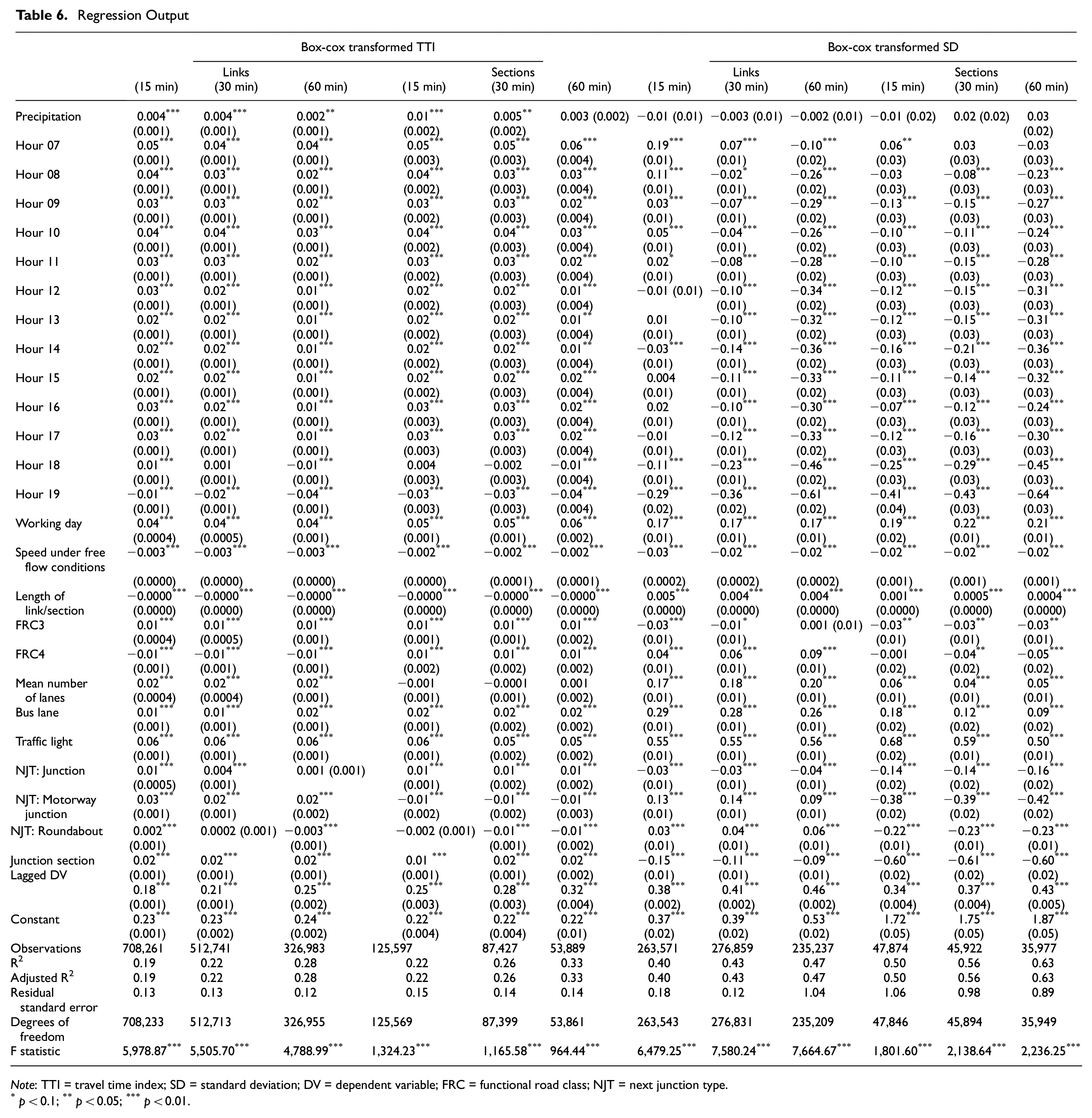
Table 6 shows the regression results for the different variants of spatial and temporal data aggregation presented in Table 1. First we analyze the influence of the IVs and how they differ between the models. Interestingly, when TTI is used as the DV, the dummy variable “precipitation” has a significant positive influence for all spatial and temporal aggregation levels except for Sec-60. On the other hand, when explaining SD, precipitation has no significant influence for any of the models. With regard to the influence of the time of the day, we find that if we take 6 a.m. as the reference category, 7 a.m. shows the strongest significant positive influence on the TTI. For SD, this picture changes, as there is a stronger negative influence on SD as the day progresses. Interestingly, we do not find clear results for 7 a.m., as the direction of the influence changes depending on the spatial and temporal aggregation used. Furthermore, the results show that there is a significant positive influence of the IV working day (Monday to Friday) on both DVs for all temporal and spatial aggregation levels compared with days on weekends. We also find that there is a significant negative relationship between the speed under free flow conditions and the TTI or SD. With regard to the length of the link or section, we find only a negligible effect on the TTI or SD. The effect of the FRC depends on whether we use the TTI or SD as the DV. For the TTI, taking FRC 2 as the reference category, the results show that FRC 3 has a significant positive impact for all levels of temporal and spatial aggregation. FRC 4 has a significant negative effect for links and a significant positive effect for sections. Interestingly, all results show an opposite effect when using the SD as the DV. The number of lanes has a significant positive effect on the DVs, except when analyzing TTI and using sections as the level of spatial aggregation. Moreover, the IVs traffic signal and buslane have a significant positive effect for all levels of temporal and spatial aggregation analyzed. Furthermore, if we analyze the influence of the next junction type a vehicle has to cross, we find, if we take complex junction as a reference category, that the type of junction has a significantly positive influence on the TTI, but a significantly negative influence on the SD. Interestingly, a motorway junction has a significantly positive effect on TTI and SD when links are used for spatial aggregation, but a significantly negative effect for sections. In addition, using junction section as a dummy variable, we find a significantly positive relationship when we use TTI, but a significantly negative relationship when we use SD as DV. However, the IV with the highest significantly positive effect on the DV is the lagged DV. Thus, the higher the DV in TOD interval t–1, the higher the DV in TOD interval t.
Regression Output
Note
Finally, the results show that the adjusted
Predictive performance of the linear regression model on test data
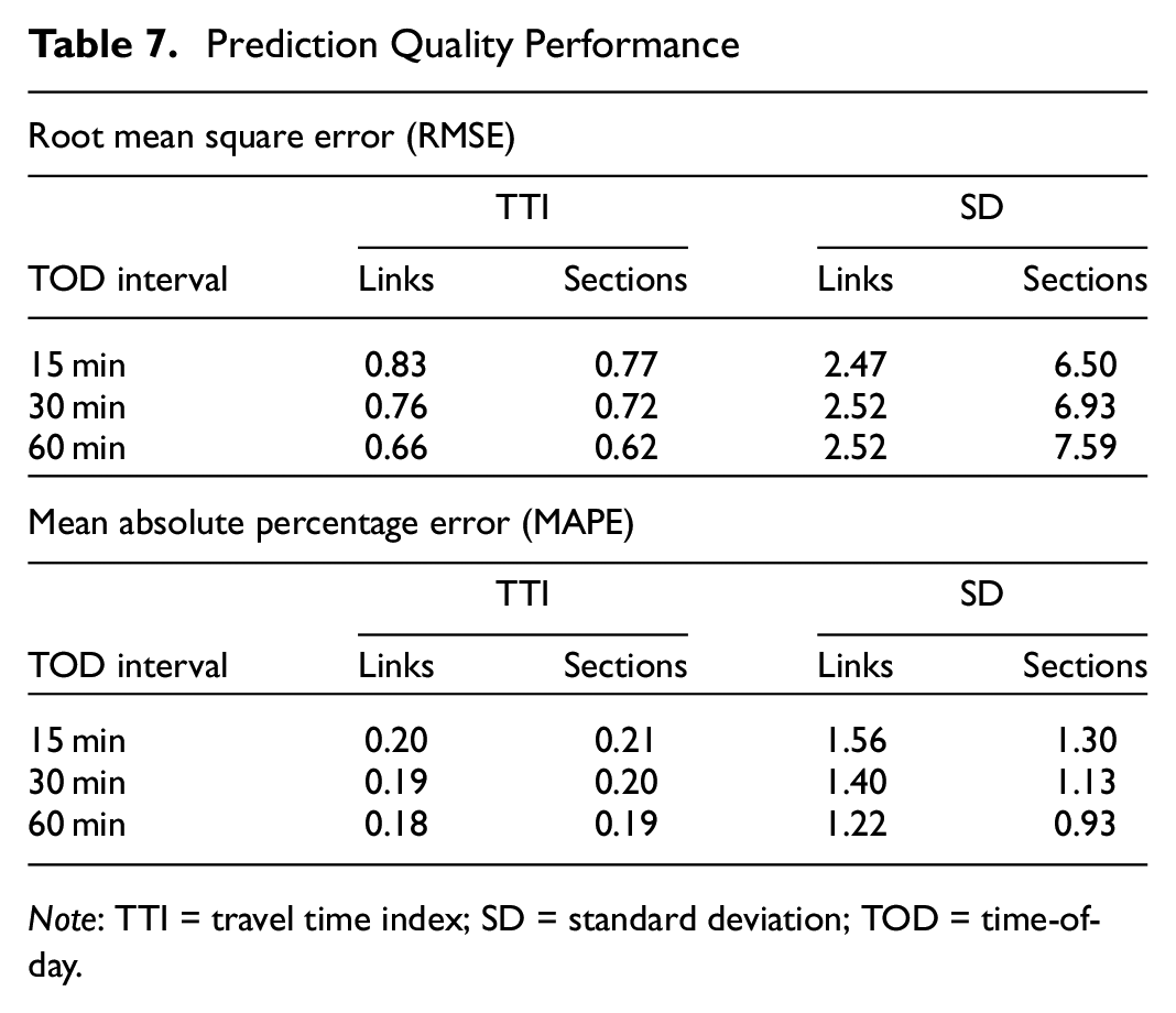
Table 7 shows the results of how well the model variants perform in predicting the DV of a test data set.
Prediction Quality Performance
Note: TTI = travel time index; SD = standard deviation; TOD = time-of-day.
In this context, we have to mention that the interpretation of the RMSE is not trivial, as we use the box-cox transformed TTI or SD as DVs. Therefore, we only evaluate the RMSE for whether it is decreasing or increasing. With respect to the TTI, the RMSE decreases with coarser temporal and spatial aggregation of the data. Interestingly, in explaining the SD, the RMSE shows an increase with coarser temporal and spatial aggregation levels of the data. When analyzing the TTI, the results show that the MAPE decreases with longer TOD intervals, but increases slightly when using sections instead of links. Furthermore, using SD as the DV shows smaller MAPEs for coarser temporal and spatial levels of aggregation of the data.
Robustness Check
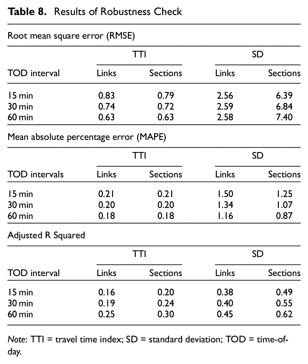
To check whether the results depend on certain seasonal patterns, we perform a robustness check, performing the analysis with training data from January 1 to February 17 and test data from February 18 to March 10, 2019. Table 8 presents that the robustness check showing similar values for the RMSE, MAPE, and the adjusted
Results of Robustness Check
Note: TTI = travel time index; SD = standard deviation; TOD = time-of-day.
Discussion
The results show that for the IVs working day, free flow speed, number of lanes, buslane, motorway junction, and the lagged DV, the same direction of effect emerges for both DVs and all analyzed temporal and spatial levels of aggregation of the data. The dummy variable working day shows a positive relationship with the DV, which means that we have a lower TTR on working days than on weekends. This finding is to be expected as it reflects the traffic congestion caused by commuters during peak hours on working days. Moreover, the volume of traffic is also lower at weekends than on working days. Interestingly, the IV free flow speed has a negative impact on TTR. Thus, the higher the free flow speed on a link or section the higher is the TTR. In addition, the results suggest that links and sections with a low free flow speed are more prone to traffic delays and have a lower TTR compared with links and sections with a higher free flow speed. Furthermore, the results show that the more lanes there are on a link or section, the higher the DV, which implies a lower TTR. We assume that if a link is already planned with more than one lane, traffic planners already assume a higher traffic volume compared with single lanes. Furthermore, if a link or section has a bus lane, the DV is higher than for links and sections without a bus lane. This finding may be because bus stops are located directly on the roadway, which means that individual traffic has to wait while the bus stops to let people on or off. In addition, the results suggest that the higher the TTR in the previous TOD (t–1), the higher it is in the TOD under consideration (t). So we assume that delays in traffic have a certain inertia and therefore tend to continue into future TOD.
Moreover, the dummy variable precipitation shows a significant effect for TTI but not for SD. This suggests that precipitation tends to increase travel time as it has a positive influence on TTI, but has no influence on the variability of travel times in a respective TOD interval on a given day. Furthermore, we find that the effect of some IVs shows different directions between the two DVs. This is especially true for variables that reflect road construction elements. With respect to the FRC and the categorical variable next junction type, we find a positive relationship when we use TTI but a negative relationship when we use SD as the DV. We may explain this phenomenon as a result of the different nature of TTR measures used in this study. Therefore, when analyzing IVs that explain TTR, future research must carefully select the particular TTR measure or, even better, run models with different measures to support the generality of the results. Given the skewness of the underlying travel time distributions, measuring TTR with an interquartile range or the planning time index could lead to a change in the influence of certain IVs and could therefore be of interest for future work. For the IVs explaining the effect of TOD on SD, we also find that the results depend on how the data are temporally and spatially aggregated. In particular, the Link-15 aggregation level shows a different pattern than the other aggregation variants. Consequently, the results indicate that too fine a temporal and spatial level of data aggregation leads to a different interpretation of the IVs which show the impact of the time of the day. Analyzing the results of the adjusted
For the predictive performance of the linear regression model on training data, we find that according to the categorization framework of Lewis (
30
) in Table 4, the MAPE shows that TTI can be predicted with good or reasonable quality, while SD is inaccurately predicted. This is interesting because, according to the results of the adjusted
However, we would like to mention that the main purpose of this analysis is not to achieve the best possible predictive performance. In this case, it would be possible to use different machine learning approaches such as neural networks ( 37 ), support vector regressions ( 38 ), or tree-based approaches ( 39 , 40 ), which can outperform the predictive performance of a linear regression. The main objective is to analyze the difference in predictive performance at different levels of temporal and spatial aggregation of the data. In combination with the other research questions, such as analyzing how the effect of IVs differs when using different temporally and spatially aggregated data sets of sparse PVD, linear regression is best suited for our purpose.
Furthermore, the robustness check shows that when applying the models to a different time period, the main conclusions of the analysis and the patterns of the results do not change.
It is worth mentioning, however, that other machine learning approaches, besides the linear regression approach, could be used to conduct the analysis. The use of tree-based methods such as random forests would allow the researcher to test the significance of the features for different spatially and temporally aggregated data sets of PVD. In addition, more sophisticated methods such as neural networks could be used to check whether the results show the same pattern for predictive performance as in linear regression. However, given the good interpretability of the results of a linear regression, we believe that this approach is best suited to answer the question of the impact of IVs on different aggregations of the data set.
Conclusion
The results of this work contribute to answering the question of whether the temporal and spatial aggregation level of sparse PVD has an impact on the results of a linear regression analysis in explaining TTR. To answer this question, we use the TTI and SD as two measures of TTR and run a linear regression when using different aggregation levels of PVD. In this context, we apply model diagnostics to all models before using them for evaluation and check the general assumptions of linear regression. In summary, the results show that with a coarser temporal and spatial aggregation of the data, a higher proportion of the variance of the DV can be explained. Therefore, we add to the literature that the proportion of the variance of the DV that can be explained by the IVs increases when longer TOD intervals and sections instead of links are used to aggregate PVD. Furthermore, we find that the effect of road construction features, in particular, depends on the variable used to represent the TTR. The results thus show that the effects of certain variables on TTR may depend on the temporal and spatial level of aggregation as well as on the TTR measurement used. Consequently, researchers and practitioners need to consider the possibility that a different level of aggregation may lead to significantly different results for the relationship between IVs and DV. In addition, our results help transport planners to better assess the impact of road design elements, temporal characteristics, and precipitation on TTR. Nevertheless, the results show that different temporal and spatial aggregation levels of the PVD should be used for deriving transport planning decisions to ensure the robustness of the results. However, when applying the trained model to a test data set to predict the DV, we do not find a clear pattern of results for appropriate temporal or spatial aggregation of the data. Therefore, future work should focus on evaluating different methodological approaches for prediction as artificial neural networks, to find new insights to this question. We would also suggest using additional IVs and different measures of TTR. This could enrich the knowledge with regard to the interdependencies between the spatial and temporal aggregation of PVD and its effect on TTR. In addition, future research could apply the proposed method to a data set with higher penetration rates and show how the results change when denser PVD is used.
Footnotes
Author Contributions
The authors confirm contribution to the paper as follows: study conception and design: S. Kranzinger, M. Steinmaßl; data collection: S. Kranzinger, M. Steinmaßl; analysis and interpretation of results: S. Kranzinger, M. Steinmaßl; draft manuscript preparation: S. Kranzinger, M. Steinmaßl. All authors reviewed the results and approved the final version of the manuscript.
Declaration of Conflicting Interests
The author(s) declared no potential conflicts of interest with respect to the research, authorship, and/or publication of this article.
Funding
The author(s) disclosed receipt of the following financial support for the research, authorship, and/or publication of this article: Federal Ministry Republic of Austria for Climate Action, Environment, Energy, Mobility, Innovation and Technology. Grant Number: GZ BMVIT-612.014/0015-III/11/2018