
Abstract
Bus rapid transit (BRT) can offer transit mobility to meet growing travel demands by cost-effectively providing high capacity and quality of service. It is adaptable to a wide range of operating conditions and technological advancements. Stations are elements that typically control BRT line capacity, so it is essential to understand the operation of any potentially critical station to understand and manage the facility. The Transit Capacity and Quality of Service Manual (TCQSM) provides the standard methodology for capacity estimation. However, that model does not account for important operational aspects including the stochastic nature of many parameters beyond dwell time, along with nonstopping buses’ capacity, the degrees of saturation of the stopping and nonstopping bus streams, and the upstream average waiting time and queue length of stopping buses. We adapted the theory developed by Hisham et al. for an onstreet bus stop, to reflect the operational conditions of a BRT station and to account for these aspects. This new reliability-based capacity model tailored to BRT facilities provided superior insight into station bus capacity and quality of service to the TCQSM model.
Bus rapid transit (BRT) systems use dedicated lanes or guideways and oftentimes advanced vehicles and technology to improve capacity, reliability, performance, and quality of service (QOS) over conventional onstreet bus (OSB) systems. One of the many advantages of BRT systems is their ability to be developed and operated economically to suit a wide range of environments. Rede Integrada de Transporte commenced service in Curitiba, Brazil in 1974 and has since inspired many high-standard BRT systems in over 44 countries worldwide ( 1 ). Because BRT systems contain features similar to a light rail or subway system, they are often considered more reliable, convenient, and faster than regular bus services ( 2 ).
The success of a BRT system is highly dependent on network topology, station typology, location, spacing, and design. Stations often provide level boarding using either low-floor buses at curb height, or higher boarding platforms. Because buses operate at higher frequencies than OSB, stations have a vital role in maintaining efficient operation through sufficient capacity and QOS.
We define a BRT line as a corridor containing multiple segments that carries one or more bus routes. We define a guideway as the actual roadway that carries the buses. Although a BRT station may have various configurations, our study is limited to a directionally separated station where buses cannot overtake across the oncoming side of the guideway. The station includes a linear platform in each direction to serve passengers. Each platform contains multiple, offline, linear loading areas (Figure 1). In each direction the guideway contains an adjacent passing lane for stopping buses to negotiate around each other when accessing or egressing loading areas, and for nonstopping buses to pass through the station.
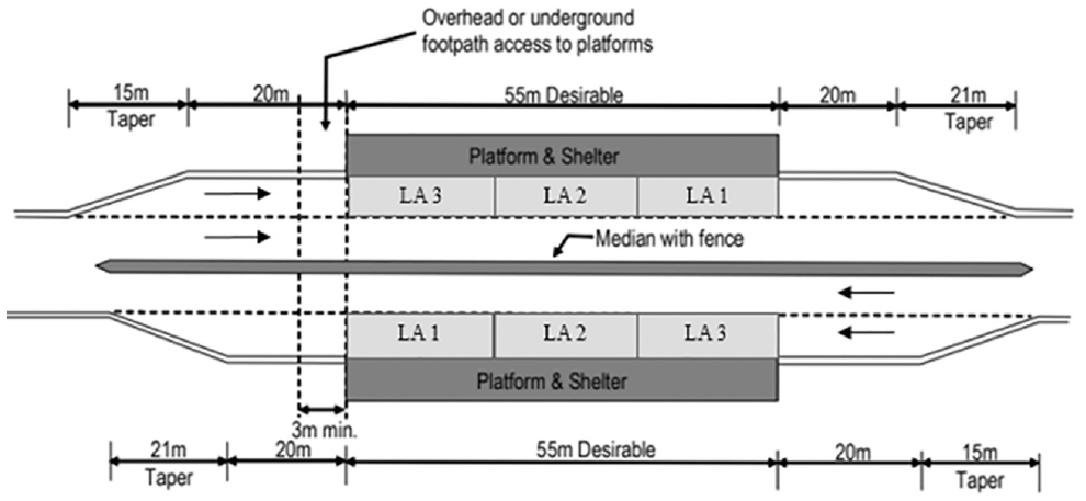
Typical bus rapid transit station layout on South East Busway, Brisbane, Australia ( 3 ).
When the adjacent lane at an OSB stop carries a high volume of general traffic, interaction between buses and nonstopping vehicles will affect vehicle capacity and QOS of the bus facility ( 4 ). Likewise, at a BRT station with nonstopping buses, it is essential to understand the operation of any potentially critical station to manage the facility.
Transit facility—or line—capacity is defined by the Transit Capacity and Quality of Service Manual (TCQSM) as the “maximum number of transit vehicles that can pass a given location during a given time period” ( 5 ). The given location is usually the critical station, which is the busiest station that causes the greatest restriction to line capacity. The period is usually a peak hour in the peak travel direction. Critical station capacity is the product of the capacity of each of its loading areas and the number of effective loading areas. A traffic blockage factor resulting from general traffic in the lane used by the buses is applicable to a stop near a signalized intersection.
The analytical model of the TCQSM methodology includes an operating margin to accommodate irregularities in buses’ dwell times. Added to dwell time, this yields the maximum amount of time that a bus can dwell on a loading area without creating a “bus stop failure.” TCQSM defines failure as a situation that arises when a bus arrives to use a loading area only to find another bus is still occupying it ( 5 ). This implies that all buses arrive at the loading area on schedule (at even headways) and that a failure is an isolated event that is remedied as soon as the bus causing the failure departs the loading area.
Bunker argued that the TCQSM model is reasonable for relatively evenly spaced arrivals between successive buses, which may be the case for a bus line with relatively widely spaced headways ( 6 ). However, for high volume bus stops—such as BRT stations—the headways between arriving buses will be stochastic because of bunching, asynchronous scheduling between routes, and platooning caused by any nearby upstream signalized intersection. Processing times on the loading area will also vary, rather than being a fixed value equal to the inverse of effective design capacity, which is a key assumption of the TCQSM model. Through simulation that incorporated this stochasticity, Bunker developed a model to estimate upstream average waiting time for stop types including BRT stations ( 6 ). This time reflects horizontal queue accumulation upstream of the station and its impact on facility performance, which the failure rate approach does not.
Hisham et al. accounted for upstream waiting time in development of the Bus Stop Maximum Working Capacity with Adjacent Lane Traffic (BMWCA) model to estimate onstreet, midblock, offline OSB capacity ( 4 ). The BMWCA model accounts for stochastic events near an onstreet, midblock, offline bus stop, which are also relevant to BRT stations, such as variability in bus arrival patterns and interference between buses caused by this. The model allocates a parameter defined as a “processing margin” for the whole stop rather than by consideration at the loading area level. It also quantifies the degree of saturation of adjacent lane traffic and maximum working degree of saturation and capacity of the bus stop as a function of specified upstream average waiting time, adjacent lane flow rate, and input parameters used in the TCQSM model ( 4 ). However, this model was developed considering a scenario of an onstreet, midblock, offline bus stop.
This study aimed to improve and extend the BMWCA model to reflect BRT station operation, to ensure that sufficient capacity is available for the nonstopping buses in the adjacent passing lane, and that upstream waiting times and queue lengths of stopping buses are maintained at acceptable levels. To achieve this aim, a literature review on bus facility capacity is provided in the next section. The Method section reviews the TCQSM model of BRT line bus capacity estimation, develops an improved model to estimate BRT line bus capacity, and details an analytical testbed to compare the TCQSM and improved models. For this testbed, the Results section details practical capacity and degree of saturation calculations, describes and evaluates the relationship between stopping buses’ maximum working capacity and nonstopping buses’ flow rate, and specifies and evaluates the relationship between stopping buses’ average upstream queue length and nonstopping buses’ flow rate. This is followed by Conclusions, which includes recommendations for further research.
Literature Review
Bus transit capacity depends on the number vehicles, the operation of vehicles, passenger and traffic volumes, and the operating policies of the transit agency ( 7 ). Two types of capacity measures are considered to measure BRT line (facility) capacity: facility bus capacity and facility person capacity ( 8 ). This study focused on bus capacity, which was estimated at the critical station considering loading area bus capacity, station bus capacity, and line bus capacity.
The Highway Capacity Manual (HCM) (
9
) introduced an empirical model to estimate BRT line bus capacity. Levinson and St. Jacques modified this equation using field studies and simulations, incorporating failure rate to estimate maximum achievable capacity (
7
). They used a coefficient of variation for dwell time of 60% and concluded that maximum achievable capacity corresponds to a 25% failure rate. Wang et al. estimated failure rate through diffusion approximation with a similar theoretical concept (
10
). Several studies determined facility bus capacity using a specific failure rate (FR). However, for a bus stop with a single loading area Gu et al. defined FR differently from any other study (
11
). For uniform bus arrivals, they assumed that bus service time follows an Erlang-k distribution. They set the ratio of bus inflow,
Some studies related facility bus capacity to bus stop location (12, 13). Others considered stochasticity and randomness in capacity estimation. Ortiz and Bocarejo estimated capacity of the Transmillenio Bogota using a VISSIM microscopic simulation model ( 14 ). They quantified the difference in capacities when randomness of bus system operations is included. Siddique and Khan used a NETSIM microscopic simulation model to evaluate BRT facility capacity in Ottawa, Canada ( 15 ). With three scenarios presented, they compared estimated capacity with the TCQSM model to highlight the importance of incorporating stochasticity.
Several studies have examined operational measures to increase facility bus capacity. Fernández used microscopic simulation to evaluate the increased performance of a divided bus stop over that of a regular, multiberth bus stop ( 16 ). Gardner et al. ( 17 ) and Germani and Szasz ( 18 ) found that dispatching buses in an ordered manner could increase capacity. St. Jacques and Levinson proposed reconfiguration of stop geometry ( 19 ).
Fernández and Planzer identified degree of saturation (volume to capacity ratio) of a bus station to be an important capacity estimation measure ( 20 ). Hidalgo et al. incorporated degree of saturation of a substop ( 21 ). They used a degree of saturation of 0.6 considering three substops with a queuing capacity of two buses at each. They found that practical capacity increased by increasing the number of substops, platforms, and queuing capacity at stations, improving operational reliability and enhancing control strategies to allow higher saturation levels.
The TCQSM model (
5
) relates FR to a desired level of operation in which dwell time is assumed to be distributed normally. TCQSM states, design capacity is effectively maximized at a failure rate of 25% and the capacity achieved with a 25% design failure rate is termed maximum capacity. Mathematically, throughput would be the highest if a constant queue of buses existed to move into a bus stop (a 100% failure rate).
We argue that the latter part of this statement should be changed to “throughput would be the highest if a constant supply of buses existed to move into a bus stop (a 50% failure rate)” because a value of the standard normal variable of 0.000 corresponds to the right tail of the standard normal distribution equal to 0.5, such that the operating margin is equal to 0 s,

where
Given the assumption of even arrival headways, under this condition a following bus would always be ready to replace a preceding bus. Whereas a 100% FR mathematically could be approached but not reached, back toward the left tail of a standard normal distribution, which would result in an extremely large, negative operating margin.
This study addresses two major gaps. First, the TCQSM model estimates station bus capacity using FR. Even though many studies have used the model including design FR, the definition of failure and its actual implications have not been sufficiently studied. Degree of saturation of a bus stop has been identified as a crucial parameter that ensures a desired level of service (LOS); however, this has not been incorporated into capacity estimations. Second, the TCQSM model implies a reduction in bus stop capacity with an increase in nonstopping buses in the adjacent passing lane flow rate owing to the bus reentry gap acceptance process. However, it does not account for the time required by nonstopping buses to pass without exceeding the practical saturation flow rate.
Method
Review of TCQSM Model of BRT Line Bus Capacity Estimation
TCQSM (
5
) defines a loading area as a section of the stop that is designated for a single bus to stop and dwell to serve passengers. This study is concerned with a BRT station whereby other nonstopping buses can pass the loading areas while buses are dwelling. Our testbed of a typical station on the BRT system in Brisbane, Australia includes a linear platform with three loading areas in series on an offline lane and no signalized intersection within influence of the station. Therefore, green time ratio (
Stopping bus capacity is equal to the product of the number of buses that can be served by a single loading area and the number of effective loading areas according to Equation 2,

where
Startup time is the time taken by a bus to start up and travel its own length and for the next bus to pull in. It is a fixed value that corresponds to the mechanical and dimensional properties of the buses.
Reentry delay is the time consumed as the stopping bus driver seeks an acceptable gap to reenter the passing lane, according to Equation 3,
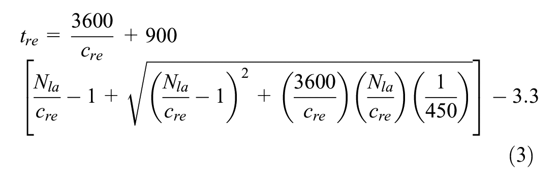
where

where
The number of effective loading areas reflects the reduction in capacity resulting from interference between buses ( 22 , 23 ). A bus stop with multiple loading areas has a greater underutilization of loading areas owing to buses interfering with each other’s ability to access or egress a loading area.
Development of Improved Model to Estimate BRT Line Bus Capacity
This development extends the BMWCA model, developed by Hisham et al. for onstreet, midblock, offline bus stops ( 24 ), to BRT operations.
Loading Area Bus Processing Time
Our BRT Facility Practical Capacity (BRT-PC) model considers loading area operation as being the fundamental building block of station operation. Loading area average total processing time per stopping bus,

where
The loading area average total processing time per stopping bus net of processing margin (s) is calculated according to Equation 6,

Hisham et al. stated that this model implies a maximum feasible degree of saturation of the bus stop (station) itself as 1.0, should a value of zero be assigned for the margin on loading area average total processing time per stopping bus ( 24 ). The margin on loading area average total processing time per stopping bus (s) is calculated according to Equation 7,

Equation 7 ensures that, on average, the loading area remains idle for a portion of total loading area processing time per stopping bus, which is equal to 1 minus a designated loading area degree of saturation,
By definition

The time used by each stopping bus to negotiate around other stopped buses in both the platform lane and the passing lane at the station area is accounted for in the term
The time available for nonstopping buses to pass during average total loading area processing time per stopping bus (s) is equal to the sum of the time components of average total loading area processing time per stopping bus, during which the bus does not obstruct the passing lane, and is calculated according to Equation 9,

An important difference between the BRT-PC and TCQSM models is that we acknowledge that when no stopping buses are present, nonstopping bus traffic has a theoretical capacity (bus/h), which we modified from research undertaken by Hisham et al. ( 24 ) according to Equation 10,

where

where
Equation 6 requires quantification of stopping bus reentry delay. The BRT-PC model incorporates the gap acceptance approach according to Equations 3 and 4. However, we acknowledge that nonstopping buses are obstructed during startup time and bus–bus interference time. Therefore, the reentering bus driver will see a compressed stream of nonstopping buses during other times. For purposes of estimating reentry delay resulting from gap acceptance, from Hisham et al.’s research ( 24 ) we adjusted nonstopping bus flow rate according to Equation 12,

Using Equations 10 and 11, adjusted nonstopping bus traffic flow rate is calculated according to Equation 13,

We substituted
The critical gap lies between the largest gap rejected by a driver and their accepted gap. Maximum likelihood is the most commonly used method of estimating population critical gap ( 25 ). However, with few rejected gaps having been observed at a BRT station, it is very difficult to estimate the population critical gap of reentering bus drivers from field data. As with follow-up headway, we considered it reasonable to adopt the TCQSM value of critical gap equal to 7.0 s at a BRT station.
From research undertaken by Hisham et al. ( 24 ) interference between stopping buses at a station may be reflected by the bus–bus interference factor according to Equation 14,

where
The additional time component toward average total processing time per stopping bus resulting from bus–bus interference (s/bus) can be estimated as a margin on the sum of the time components of loading area average processing time per stopping bus, excluding the processing margin, according to Equation 15,

The system of Equations 6–15 allows us to determine loading area average total processing time per stopping bus, and the time available for nonstopping buses to pass during this time, provided that all inputs are specified. Assuming all loading areas on the platform are utilized equally, each of these time components—and their total—apply to each of the loading areas.
Startup time and average dwell time are typically analysis inputs. However, according to Equation 13, we must know nonstopping buses’ degree of saturation to determine stopping bus reentry delay. The additional time component toward average total processing time per stopping bus resulting from bus–bus interference (s/bus) can then be determined directly using Equation 15. Further, according to Equation 8, we must know the loading area degree of saturation to calculate the processing margin. Therefore, these two degrees of saturation must be input to solve the whole system of equations. These inputs will now be addressed.
Relationship between Stopping Buses’ Practical Capacity and Nonstopping Buses’ Flow Rate
To further develop the BRT-PC model it is useful to establish the relationship between stopping buses’ practical capacity and nonstopping buses’ flow rate. We define practical degree of saturation as the greatest value that maintains acceptable, uncongested operation.
First, we determine nonstopping buses’ practical capacity, which occurs at a frontier where both nonstopping buses reach their practical degree of saturation,
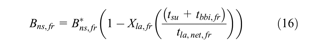
where nonstopping buses’ practical maximum flow rate,
Second, we determine nonstopping buses’ degree of saturation for any given nonstopping buses’ flow rate,
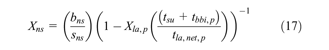
This formula is the quotient of the nonstopping buses’ flow ratio and the probability that the loading area is not jointly occupied and causing blockage on the passing lane at practical saturation.
Nonstopping buses’ degree of saturation,

where a suitable initial trial value for the argument is
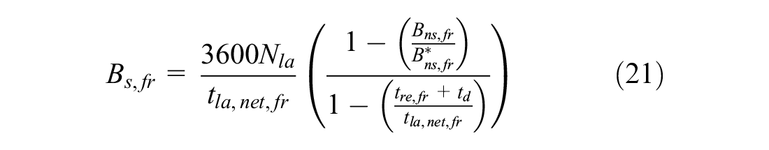
Stopping buses’ practical capacity for the given nonstopping bus flow rate is then calculated according to Equation 19,

Practical Saturation Frontier
Equation 16 reflects that operation of the station is limited by a practical saturation frontier, which we can further define as the relationship between nonstopping buses’ practical capacity and stopping buses’ practical capacity.
The theoretical minimum possible value of

The relationship for stopping buses’ practical capacity on this frontier, where
Station operation on the practical saturation frontier would be highly volatile and is therefore not recommended.
Suitable Nonstopping Buses’ Practical Degrees of Saturation
Equations 16–19 require specification of loading area practical degree of saturation,
First, we considered nonstopping buses’ practical degree of saturation. If this value is considered constant across all flow rates less than practical capacity, operating degree of saturation will be less than practical degree of saturation.
The general traffic facility that most closely approximates a BRT facility where buses cannot overtake is a two lane, two-way directional segment. HCM 2016 ( 26 ) stipulates a typical saturation flow rate of 1,700 passenger cars per hour (pcph) and contains a method to determine LOS at this type of facility, which is based on estimation of percent time spent following and average travel speed considering both directions of travel, given the directional flow rates. However, this method is not suited to the low travel speed environment of a BRT facility at a station, where a posted speed limit of 50km/h applies in our testbed. Regardless of flow rate and estimated percent time spent following, the method returned a LOS E performance and was therefore unable to be used to define a suitable practical degree of saturation.
We instead considered the HCM 2016 (
26
) multilane highways method to estimate saturation flow rate and practical degree of saturation, using the speed–flow curves with LOS criteria on a per lane basis. On the Brisbane, Australia BRT network that is represented by our analytical testbed, nonstopping bus drivers are trained to pass a BRT station without exceeding the 50 km/h posted speed limit. The HCM method does not contain a curve for this value as free flow speed. However, extrapolation from the family of speed–flow curves indicates a capacity of 1,500 passenger cars per hour per lane (pcphpl) for a 50 km/h free flow speed. The method recommends a heavy vehicle adjustment of 1.5 pc, so the extrapolated theoretical capacity and therefore saturation flow rate on the passing lane,
Suitable Loading Area Practical Degree of Saturation
Second, we considered loading area practical degree of saturation. Along with its value, the assumption about whether loading area practical degree of saturation should remain constant with nonstopping buses’ flow rate requires careful consideration. Bunker discussed that processing of buses through a loading area of a bus stop has similar characteristics to the operation of an unsignalized intersection ( 6 ). However, the loading area as a server is subject to less fluctuation than the head of the queue on a minor movement at an unsignalized intersection. The increase in upstream average waiting time with degree of saturation were noted as being less pronounced. However, waiting time upstream of a loading area at a BRT station can be more consequential than at an unsignalized intersection, because of the effects of bus queuing on station and line operations.
Bunker estimated upstream average waiting time according to Equation 22 ( 6 ),
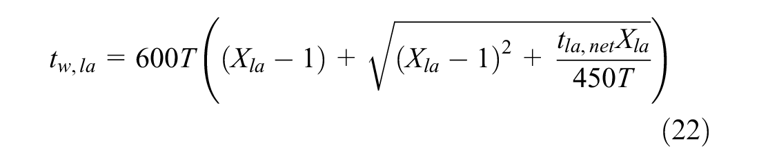
where system time
Rearranging Equation 22, an appropriate loading area practical degree of saturation assuming common utilization across all loading areas can be defined according to Equation 23,

where
Loading area practical degree of saturation should not cause excessive upstream average waiting time, particularly as nonstopping buses’ flow rate approaches practical capacity. To determine nonstopping buses’ practical capacity and the associated loading area practical degree of saturation, we considered specified upstream average waiting time values of between 10 s and 30 s.
To further investigate the effect of specified upstream average waiting time, we estimated stopping buses’ average queue length upstream of the station platform according to Equation 24,

Charting Practical Saturation Frontier
To chart the practical saturation frontier, we estimated the range of loading area practical degree of saturation using Equations 20 and 21 by varying
Flowcharts
The left-hand panel in Figure 2 illustrates the flowchart to estimate stopping buses’ practical capacity and average upstream queue length as a function of nonstopping buses’ flow rate and other necessary parameters; the right-hand panel illustrates the flowchart to chart the practical saturation frontier, using the BRT-PC model.
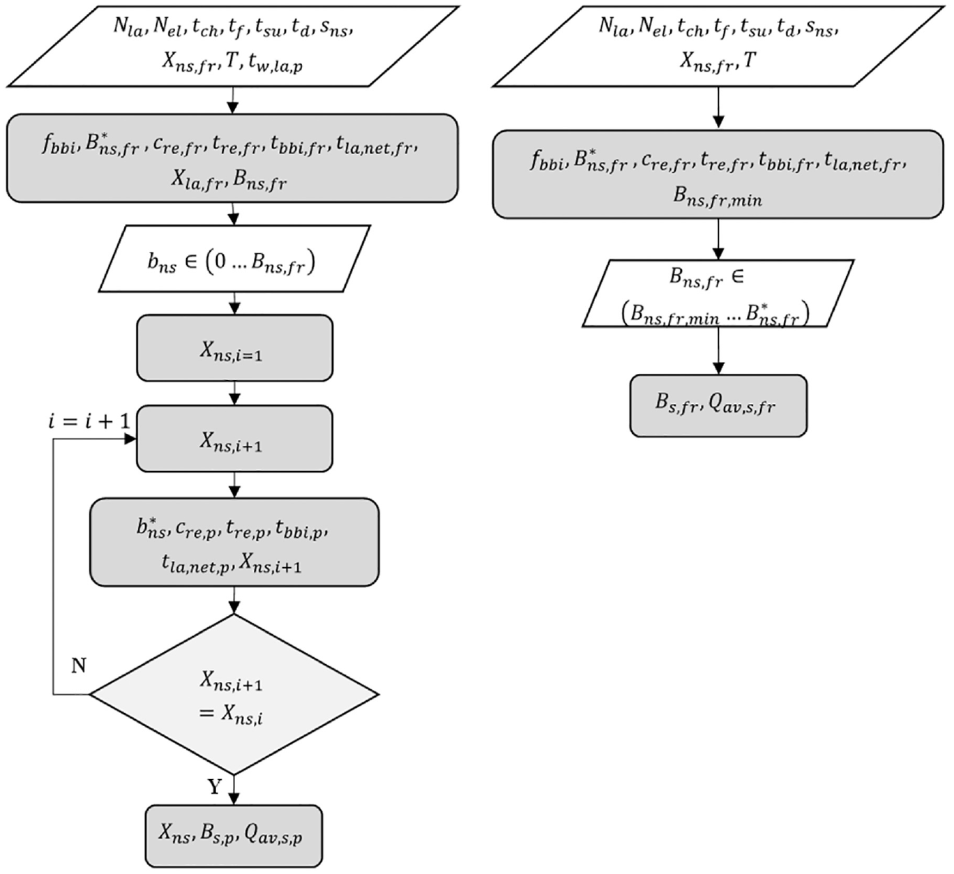
Bus rapid transit facility practical capacity model estimatation of stopping buses’ practical capacity and average upstream queue length (left panel) and practical saturation frontier (right panel).
Analytical Testbed to Compare TCQSM and BRT-PC Models
For direct comparison, we determined the capacity of a stylized station on the Brisbane, Australia BRT network using the TCQSM model based on Equation 2 and the BRT-PC model of Equations 5–24 under conditions where nonstopping buses have absolute priority over reentering buses. We used a peak period mean dwell time of 20 s ( 6 ) to reflect a typical BRT station. We assigned the startup component of clearance time equal to 10 s for a standard bus ( 27 ). We estimated reentry delay using values of 7.0 s for critical headway and 3.3 s for follow-up headway. The testbed BRT station contains three actual loading areas. We used a value of 2.60 effective loading areas according to TCQSM ( 5 ). The next section presents the results.
Results
Nonstopping- and Stopping Buses’ Practical Capacity and Degree of Saturation Calculations
Using Equations 3 and 4, reentry delay,
For an example specified practical upstream average waiting time of 20 s, using Equation 23, loading area practical degree of saturation,
We used the left-hand flowchart of Figure 2 to determine stopping buses’ practical capacity and degree of saturation, as well as nonstopping buses’ degree of saturation, across a range of nonstopping buses’ flow rates,
Stopping Buses’ Practical Capacity versus Nonstopping Buses’ Flow Rate
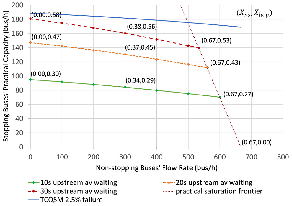
The relationship between stopping buses’ practical capacity and nonstopping buses’ flow rate using the BRT-PC model for prescribed upstream average waiting times of 10 s, 20 s, and 30 s, along with TCQSM model results for a conservative FR of 2.5% are illustrated in Figure 3. TCQSM recommends this value of design FR outside downtown areas “whenever possible, particularly when offline stops are provided, as queues will block a travel lane whenever a bus stop failure occurs” ( 5 ).
Testbed BRT station stopping buses’ practical capacity versus nonstopping buses’ flow rate (BRT-PC and TCQSM models).
The BRT-PC model curve is shown in Figure 3 for each prescribed upstream average waiting time. As nonstopping buses’ flow rate increased, both reentry delay and bus–bus interference time increased, leading to an increase in loading area average total processing time per bus net of processing margin, and a gradual decrease in stopping buses’ practical capacity and degree of saturation.
The practical saturation frontier is also shown, which was calculated using the right-hand flowchart of Figure 2. Stopping buses’ practical capacity and degree of saturation reduced linearly, and dramatically so, to a value of zero when nonstopping buses’ flow rate reached maximum practical,
Stopping buses’ practical capacity and degree of saturation were affected markedly by prescribed upstream average waiting time. For instance, when there are no nonstopping buses, by limiting upstream average waiting time to 10 s, the loading areas will operate at a practical degree of saturation of 0.30, whereas by limiting the average waiting time to 30 s, the loading areas will operate at a practical degree of saturation of 0.58. This demonstrates the importance of setting an appropriate upstream average waiting time.
The relationship between stopping buses’ design capacity and nonstopping buses’ flow rate using the TCQSM model under a 2.5% FR was similar to the BRT-PC curve for a 30 s upstream waiting time under a low nonstopping buses’ flow rate, but did not decrease with increasing nonstopping buses’ flow rate as much as the BRT-PC model, because the TCQSM model does not account for the compressed nonstopping buses’ flow rate witnessed by reentering drivers.
On the practical saturation frontier, the effect of increasing the processing margin dramatically reduced stopping buses’ practical capacity toward zero at nonstopping buses’ maximum practical flow rate. With this sharp reduction, operation was highly volatile with nonstopping buses’ flow rate and needs to be avoided. However, the TCQSM model does not account for this frontier at all. This comparison demonstrates that both phenomena are significant in BRT station operation.
Figure 3 highlights that under the conservative 2.5% FR, the TCQSM model stopping buses’ design capacity was approximately twice the practical capacity estimated using the BRT-PC model for a specified 10 s upstream average waiting time. This highlights that the TCQSM FR approach does not account for the significance of the effect of cascading delays resulting from horizontal queue formation as buses wait to enter available loading areas, because of the stochasticity of parameters discussed earlier and in research by Hisham et al. ( 4 ).
Stopping Buses’ Average Upstream Queue Length versus Nonstopping Buses’ Flow Rate
To investigate the effect of prescribed upstream average waiting time further, we estimated the stopping buses’ average upstream queue length using Equation 24. Figure 4 illustrates the relationship between this queue length and nonstopping buses’ flow rate using the BRT-PC model for prescribed upstream waiting times of 10 s, 20 s, and 30 s.
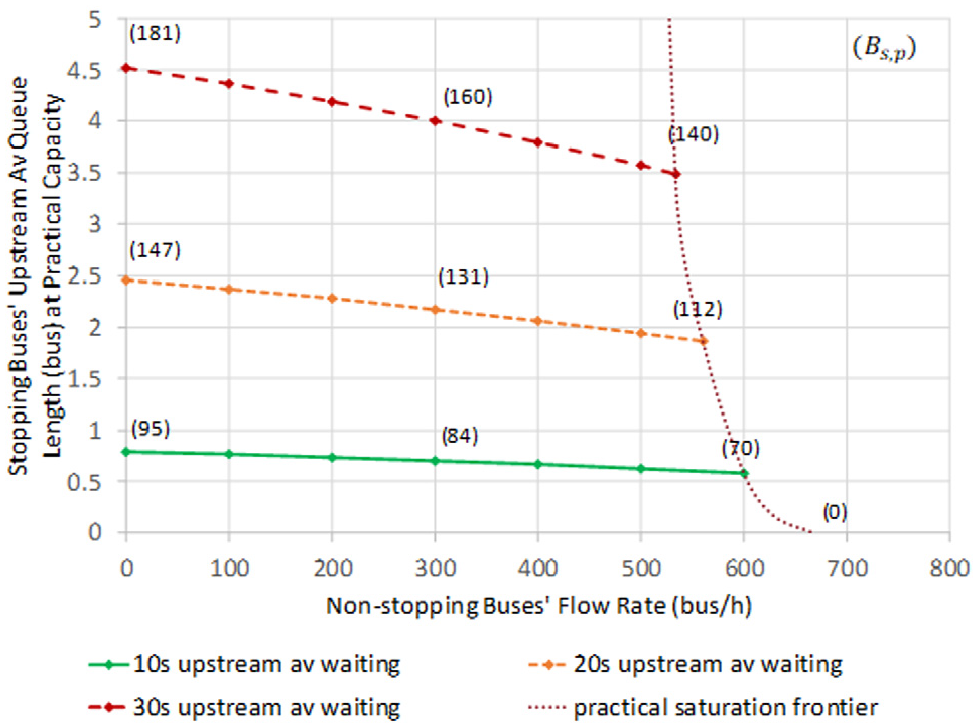
Testbed BRT station stopping buses’ upstream average queue length at practical capacity versus nonstopping buses’ flow rate (BRT-PC and TCQSM models).
Stopping buses’ upstream average queue length was affected profoundly by prescribed upstream average waiting time. For a given nonstopping buses’ flow rate, upstream average queue length for a 20 s upstream waiting time was approximately three times that of a 10 s average waiting time, whereas average queue length for a 30 s upstream waiting time was approximately six times that of a 10 s average waiting time. It is crucial to prescribe a stopping buses’ upstream average waiting time that does not cause excessive bus queues that spill out of the stopping lane upstream of the platform and diverge taper, into the passing lane.
For stations on the Brisbane, Australia BRT network represented by the analytical testbed, the stopping lane typically extends 20 m back from the rear of the platform (Figure 1). The diverge taper length varies depending on approach speed. The 20 m stopping lane extension plus a portion of the diverge taper that accommodates a bus width of 2.4 m would hold a queue of just two 12.3 m rigid buses. According to Figure 4, a prescribed upstream average waiting time of 10 s would result in a stopping buses’ upstream average queue that would readily be stored in the available geometry, without blocking nonstopping buses. However, a prescribed upstream average waiting time of 20 s would result in queuing that would, on average, block nonstopping buses, which may be unacceptable, especially on higher speed approaches. Under such circumstances, a prescribed upstream average waiting time of 30 s would clearly be unacceptable.
It is noteworthy that stopping buses’ upstream average queue length reduced moderately as nonstopping buses’ flow rate increased. This was because of the moderate reduction in stopping buses’ practical capacity and its direct effect on average upstream queue length according to Equation 24.
On the practical saturation frontier, stopping buses’ upstream average queue length reduced sharply toward zero at the point where nonstopping buses’ maximum practical flow rate was reached, corresponding to zero working capacity for stopping buses. Again, with this sharp reduction, operation was highly volatile with nonstopping buses’ flow rate and needs to be avoided.
This examination of stopping buses’ upstream average queue lengths considered horizontal queuing. It is important to note that, at times when queues exceed the average, additional geometry may be necessary to store nonstopping buses mixed in a queue. It may be appropriate to consider a stopping buses’ upstream design queue length, or a more conservatively prescribed upstream average waiting time to avoid nonstopping buses from being queued.
Estimation of this upstream bus queuing was not possible using the TCQSM model. This examination highlights the need for our BRT-PC model to analyze and design for this crucial aspect of BRT station operation.
Conclusions
Our study developed the BRT-PC model to estimate BRT station stopping buses’ practical capacity as a function of nonstopping buses’ flow rate as well as the traditional parameters of the TCQSM model. By associating a practical saturation frontier with nonstopping buses, reflecting that reentering drivers witness a compressed nonstopping buses’ stream, and incorporating stopping buses’ practical degree of saturation as a function of prescribed upstream average waiting time, the BRT-PC model provided superior insight into station operation to the TCQSM model. We related stopping buses’ practical degree of saturation directly to the processing margin, which, unlike the TCQSM model operating margin, accommodates all stochastic influences that may arise during the processing of a stopping bus.
We quantified nonstopping buses’ practical saturation flow rate and practical degree of saturation by considering the analogous system of a low speed, multilane highway lane operating at a LOS D/E threshold. Our BRT-PC model estimated stopping buses’ practical degree of saturation as a function of a prescribed upstream average waiting time by considering the analogous system of delay at an unsignalized intersection minor movement.
We applied an analytical testbed based on a stylized station of the BRT network of Brisbane, Australia, illustrated in Figure 1 to compare the results using the TCQSM and BRT-PC models with typical values of input parameters. The relationship between stopping buses’ design capacity and nonstopping buses’ flow rate estimated according to the TCQSM model under a conservative 2.5% FR was similar to the BRT-PC curve for a 30 s upstream average waiting time under low nonstopping bus flow rates, but did not decrease with nonstopping bus flow rate as much as the BRT-PC model, highlighting that the FR approach does not account for the numerous stochastic influences that result in the significant effect of cascading delays owing to horizontal queue formation as buses wait to enter available loading areas.
The BRT-PC model revealed that stopping buses’ practical capacity and degree of saturation were affected markedly by prescribed upstream average waiting time. To investigate this further, we estimated stopping buses’ upstream average queue length. When nonstopping buses’ degree of saturation was less than the practical limit, stopping buses’ upstream average queue length was affected profoundly. For a given nonstopping buses’ flow rate, average queue length for a 20 s upstream waiting time was approximately three times that of a 10 s average waiting time, whereas average queue length for a 30 s upstream waiting time was approximately six times that of a 10 s average waiting time.
It is crucial to prescribe a stopping buses’ upstream average waiting time that does not cause excessive queues that spill back into the passing lane. For a 20 s average dwell time, we found that a 10 s value would result in an average queue that would readily be stored in the available geometry, without blocking nonstopping buses. However, a 20 s value would result in an average queue that would block the passing lane, which may be unacceptable, especially on higher speed approaches. A 30 s value would be clearly unacceptable.
Accurate estimation of upstream bus queuing was not possible under the TCQSM model. This highlights the need for our BRT-PC model to analyze and design for this crucial aspect of BRT station operation, which is a daily occurrence at several busy stations on the BRT network of Brisbane, Australia.
A limitation of this study was that we assumed absolute priority of nonstopping buses over stopping buses during the reentry process in our testbed analysis and comparison. Future research will examine how shared priority could be modeled effectively and whether this makes a difference to station operation. Another limitation is that we are yet to consider queuing impacts on nonstopping buses when nonstopping bus queues exceed available storage, along with the specification of design upstream queue length. Also, we directly applied the value of the number of effective loading areas from the TCQSM, which does not account for platooned arrivals or processing of offline loading areas. It would be useful to investigate further whether platooning affects station performance.
This study was limited to the standard station configuration of the Brisbane BRT network illustrated in Figure 1 comprising three offline loading areas. It would be reasonable to assume we could directly apply our BRT-PC model to stations containing either two or four offline loading areas; however, the model in its present form is not applicable to online configurations.
It will be appropriate to acquire field data across a range of BRT station types and regions globally to verify the BRT-PC model with upstream average waiting time under a wide range of operating conditions and to compare the results with those determined using the TCQSM model, to inform recommendations in relation to any revisions or additions to the TCQSM methodology.
Footnotes
Acknowledgements
The authors acknowledge the TransLink Division of the Queensland Department of Transport and Main Roads, Australia, for allowing us to observe the operation of its busway system.
Author Contributions
The authors confirm contribution to the paper as follows: study conception and design: J. M. Bunker, F. Hisham; data collection: F. Hisham, J. M. Bunker; analysis and interpretation of results: J. Bunker, F. Hisham; draft manuscript preparation: J. M. Bunker, F. Hisham. All authors reviewed the results and approved the final version of the manuscript.
Declaration of Conflicting Interests
The author(s) declared no potential conflicts of interest with respect to the research, authorship, and/or publication of this article.
Funding
The author(s) disclosed receipt of the following financial support for the research, authorship, and/or publication of this article: This research was funded in part by a QUT Write Up Scholarship.
Data Accessibility Statement
This article adapted existing theory as noted and cited, as part of the development of new theory. All data used were adapted from existing theory as cited in the Method section. All output in the Results section is directly reproduceable by applying the theory as documented.