
Abstract
This study represents an advanced approach to road weather information system (RWIS) network planning. Here, a methodological framework is developed to determine optimal RWIS locations by integrating two analysis domains: space and time. Using a case study, the application of the proposed method is demonstrated using three critical RWIS variables: air temperature, road surface temperature, and dew point temperature. With these three variables, a series of geostatistical semivariogram analyses are performed to construct a single spatiotemporal model named joint semivariogram, which is able to preserve both spatial and temporal aspects. The constructed joint semivariogram is then used to find the optimal RWIS locations for a randomly generated study area using a popular heuristic algorithm—spatial simulated annealing. The proposed method enhances the previously developed RWIS location allocation model by considering both spatial and temporal components of multiple variables. The finding from this analysis reveals that optimal RWIS location strongly depends on the spatiotemporal autocorrelation structure of the variable of interest. Consequently, location solutions generated using the three variables are found to be different from each other. The variation among the RWIS location solutions is then further quantified by developing a spatial similarity index that is used to measure the degree of spatial similarities between different variables. Overall, the findings documented in this study will provide RWIS planners with a more complete and conclusive location allocation strategy and can act as a decision support tool for long-term RWIS network planning.
Adverse climatic conditions and an increasing number of weather-related road incidents persist as vital and challenging issues in cold regions. As an important part of modern transportation engineering, intelligent transportation systems (ITS) play an essential role in our everyday life by improving transportation safety and mobility through minimizing weather-related road crashes. Road weather information systems (RWIS)—a critical part of ITS infrastructure—contain advanced sensors that collect, process, and distribute road weather and condition information like air and road surface temperatures, dew point temperature, atmospheric pressure, windspeed, and many others ( 1 ). RWIS information is often disseminated to transportation agencies to assist them in providing a timely and proactive response to severe winter weather events. Additionally, RWIS information is also used for generating dynamic message signs, websites, and services to provide road users with road condition information ( 1 , 2 ). Because of the numerous benefits associated with RWIS stations, many North American transportation agencies have invested millions of dollars to deploy additional RWIS stations on their road network to improve winter road monitoring coverage ( 1 , 3 ). However, because of the significant costs associated with installation and maintenance, it is essential to determine the RWIS siting locations that can maximize the monitoring coverage of the entire network.
Several studies were conducted in the past to establish proper guidelines for RWIS installations ( 3 – 8 ). The most notable of these was an initiative taken by the U.S. Federal Highway Administration (FHWA), which aimed at providing a standard for RWIS network planning that is dependent on the knowledge and experience of field operators ( 4 ). Besides installation guidelines, several studies were performed to build an innovative methodological framework for identifying optimal RWIS locations by generating a more objective way of quantifying the spatial coverage of RWIS data. A GIS-based framework was proposed by Kwon and Fu ( 5 ) to evaluate RWIS locations in Ontario, Canada by modeling local road weather conditions (i.e., variability of road surface temperature, mean surface temperature, and snow water equivalent) and topographic location attributes. An approach based on cost–benefit was used by Zhao et al. ( 8 ) to determine the optimal locations of RWIS by maximizing spatial coverage considering the standard deviation of weather severity. Another attempt was made by Jin et al. ( 6 ), who proposed a location optimization method that maximized spatial coverage of existing RWIS sensors based on weather-related crash data, which was converted into a safety concern index. In a more recent study, Kwon et al. used advanced geostatistical analysis to generate a methodological framework for determining the underlying spatial structure of RWIS measurements. In this research, an efficient combinatorial optimization algorithm, spatial simulated annealing (SSA) was used to perform an RWIS network location allocation analysis. The optimization was formulated as a nonlinear integer programming (NIP) problem to maximize monitoring capability while minimizing kriging errors ( 3 ).
While the above discussed literature has contributed to advancing RWIS location models, the studies so far suffer from several limitations. First, optimal RWIS locations were generated by investigating the spatial characteristics of one single RWIS variable, road surface temperature (RST). Although RST is an important measurement, RWIS provide many other weather variables that need to be considered alongside. Measurements like AT (air temperature) and DPT (dew point temperature) are just as critical in forecasting road weather conditions (for example, generation of black ice). Second, previous studies dealt solely with spatial domain of a single RWIS variable, which does not account for inherent temporal correlation of weather and road surface conditions. And since the weather parameters vary over space and time, it is essential to investigate both the spatial and the temporal variability of the variables of interest.
Spatiotemporal semivariogram analysis is an advanced geostatistical method that is used to evaluate spatial and temporal dependency of parameters that tend to fluctuate over space and time (e.g., road weather variables). This method works by combining spatial and time-series analysis to preserve the interactive effect of time variation on spatial domain and vice versa, allowing for the visualization of the spatiotemporal variability in the variable of interest and the determination of autocorrelation range over space and time. For this reason, spatiotemporal analysis has been established as more accurate than spatial analysis alone ( 9 ). Recently, a small handful of studies used the above-mentioned technique in their research. Several pieces of research used the underlying techniques to model air pollutants by measuring the space–time variability of certain particles’ concentrations ( 9 – 12 ). Hu et al. ( 13 ) applied spatiotemporal regression kriging to predict precipitation using moderate-resolution imaging spectroradiometer (MODIS) and normalized difference vegetation index (NDVI) data. In the field of transportation, the usage of spatiotemporal data has been noticed recently for evaluation of spatiotemporal outliers and the identification of erroneous sites ( 14 ); traffic accident prediction using a deep learning approach ( 15 ); and several others. One notable study related to the topic of interest is the investigation of spatiotemporal variability of road weather and surface conditions using RWIS data from Alberta, Canada ( 16 ). The output of this study provided both spatial and temporal features of the RWIS database. Although the findings were well received, there still a need for research to combine spatial and temporal variability to generate a single spatiotemporal model by preserving both space and time attributes. Moreover, spatiotemporal analysis has never been taken into consideration in the location allocation optimization of RWIS.
Therefore, the main objective of this study is to develop a methodological framework to optimize RWIS location by considering both spatial and temporal variability of multiple weather variables. The problem was formulated on the basic premise that data from RWIS stations within a region should be collectively used to maximize their overall monitoring quality. By considering multiple variables, this study will evaluate the spatiotemporal autocorrelation structure of these variables and examine their effects in generating optimal location solutions and their spatial similarities.
Methodology
Overview of Research Procedures
The first phase of this study involves analyzing spatiotemporal correlation of RWIS measurements, followed by RWIS location optimization using semivariogram parameters. Three different variables of interest are used in this study; namely, Air Temperature (AT), Road Surface Temperature (RST) and Dew Point Temperature (DPT). The raw RWIS measurements are extracted from the RWIS database, and are then checked using the following steps: data completeness test, reasonable range test, and a neighborhood value comparison. Once the data has been checked, the RWIS data is detrended with respect to time using a generalized additive model (GAM), followed by statistical analysis using descriptive statistics and correlation analysis. In the second stage, one of the most comprehensive spatial sampling techniques, called geostatistical analysis, is employed in conjunction with geographically distributed data. This technique maximizes the probability of capturing the spatial and temporal variations of the RWIS variables and minimizes the potential bias associated with input data. More specifically, spatiotemporal analysis is performed by constructing empirical variograms from processed data, which optimizes parameter estimations for unsampled locations and captures the possible autocorrelation associated with the RWIS variables. Joint semivariogram models are then developed by combining spatial and temporal semivariograms. Finally, a model-based approach via kriging is utilized in the final stage to obtain unbiased estimates with the lowest variance (i.e., uncertainty) to determine the optimal RWIS locations. The study is concluded by generating three sets of optimal RWIS locations and performing a similarity analysis. Research procedures for this study are summarized in Figure 1.
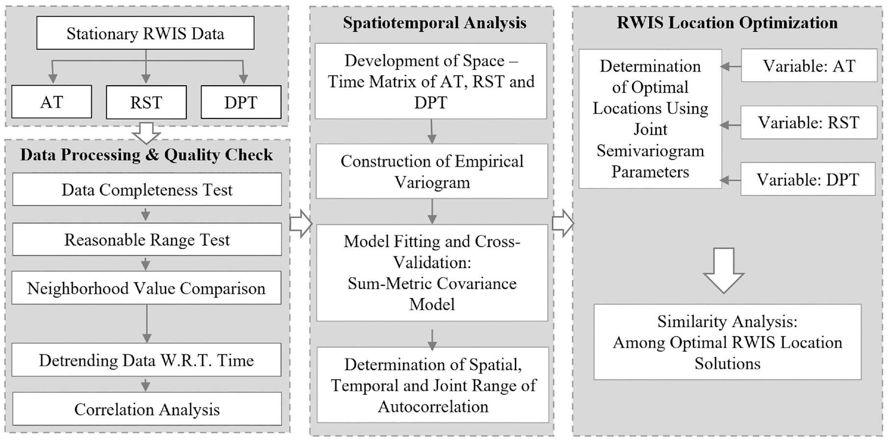
An overview of the research procedure.
Data Quality Diagnostics
Downloaded RWIS data is processed to remove missing and erroneous data. All three types of data are cross checked with one another to search for outliers. After that, data completeness is checked by identifying the total amount of missing data for each sensor—any stations with more than 15% of missing data are not used in this study. Following this, reasonable ranges of each variable under investigation are checked based on historical data ranges for the associated region and month. Filtered data is then used for pattern analysis by plotting the day of the month versus average daily temperature for all selected sensors, all weather parameters, and all months. All selected sensors for a specific weather parameter are expected to show a similar pattern throughout the month. If any unusual pattern is noticed for a specific station, the associated data is further investigated. In total, six sets of data (two months for three weather parameters) are analyzed in this study. At the end of data processing, AT, RST, and DPT data is de-trended with respect to time using a GAM to incorporate shorter scale variation in the temporal domain. Here, GAM works as a generalized linear model with linear predictors. The GAM function is formulated as
Spatiotemporal Semivariogram Analysis
Spatiotemporal analysis is generally conducted for variables that vary over space and time. In this study, spatial and temporal continuity analysis for weather variables is performed using geostatistical spatiotemporal semivariogram modeling. The traditional spatial analysis conducted in our previous efforts is incorporated with temporal analysis to consider spatiotemporal effects.
Spatial semivariogram is a graph of semivariance versus lag separation distance between pairs of measured points. Semivariance can be defined as a measure of dissimilarity between two measurements as a function of separation distance. The semivariogram has three basic parameters: nugget, sill, and range. Nugget represents measurement or sampling error; it can be defined as dissimilarity with zero separation distance, which is theoretically zero. Sill is the semivariance value at which the semivariogram levels off. The difference between sill and nugget is called partial sill and this value is often encountered during semivariogram analysis. The distance at which the semivariogram reaches the sill value is defined as the spatial range of autocorrelation, where there is no correlation among the measurements beyond this spatial range ( 18 – 21 ). A typical semivariogram with its parameters is presented in Figure 2a.
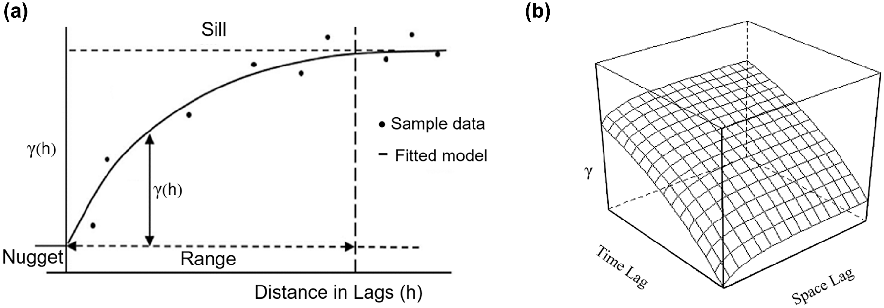
A typical: (a) semivariogram and (b) spatiotemporal semivariogram.
Spatiotemporal semivariogram modeling, on the other hand, is conducted by integrating both spatial and temporal effects of regionalized random variables (e.g., road weather). Generally, a set of variables in a spatiotemporal field can be defined as
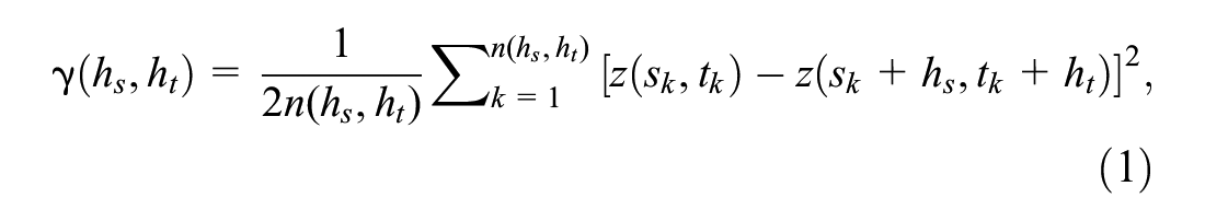
where γ(hs,ht) = estimated semivariance value, n(hs,ht) = total number of pairs in analysis domain, and z(sk,tk) = measurement at spatial location sk and temporal location tk ( 22 , 23 ). A three-dimensional spatiotemporal semivariogram is presented in Figure 2b.
After constructing the empirical variogram, a mathematical model is used to smoothen the graph by resolving the irregular pattern. There are several covariance models used for spatiotemporal semivariogram modeling ( 9 , 24 – 26 ). The most popular and widely used covariance models are: (a) separable covariance model, (b) product-sum covariance model, (c) metric covariance model, (d) sum-metric covariance model, and (e) simple sum-metric covariance model. According to previous studies, the sum-metric model performs better in fitting the spatiotemporal variogram using environmental parameters (i.e., smallest mean squared errors) ( 11 , 13 ). For this reason, the sum-metric covariance model was selected in this study. This model is a combination of spatial, temporal, and metric models. The equation for a covariance function of a sum-metric model is presented in Equation 2.
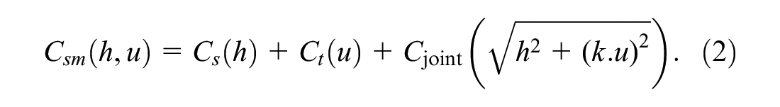
Here, h and u represent the spatial and temporal components respectively; k is a spatiotemporal anisotropy parameter. Similarly, the equation for a sum-metric variogram is given in Equation 3.
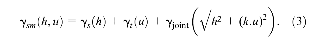
Spatial, temporal, and joint nugget are estimated separately in this model. A spatiotemporal anisotropy parameter (StAni) is used to create the joint semivariogram by combining the spatial and temporal semivariance. The number of space units equivalent to one time unit is defined as StAni. RMSE (root mean square error) is used in this study to measure the goodness-of-fit of the resultant model.
Location Allocation via Spatial Simulated Annealing
An innovative RWIS location modeling framework was developed in our previous efforts where the problem was formulated as an integer programming problem with the objective of minimizing the spatially averaged kriging variance (in other words, maximizing spatial coverage) across the road network ( 3 , 7 , 27 , 28 ). For the first time in the literature, the method developed there provided decision makers with a tool needed to optimize and expand their existing RWIS networks.
In this study, a more refined location optimization model is proposed by integrating joint semivariogram parameters generated for different weather variables to represent their distinctive spatiotemporal characteristics. Similar to our previous studies, the objective function is again formulated to minimize the sum of mean ordinary kriging (OK) estimation variance. The equations of the objective function and its related computation process are shown below.
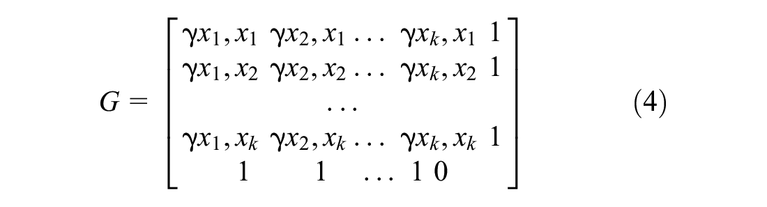
where

where

Based on the above three equations, the objective function of this work can be formulated as

subject to
The RWIS location modeling being tackled here requires mathematical and computational methods to find optimal solutions for an objective function, which is usually performed under some form of constraints. For a larger-sized optimization problem, a heuristic algorithm is an effective method for finding the solutions ( 29 ). The optimization method implemented in this study is SSA, which is a spatial counterpart to simulated annealing (SA) ( 7 , 30 ). SSA is a popular heuristic algorithm used to solve spatial optimization problems ( 7 , 31 – 34 ). SSA works by slightly perturbing previous sampling designs using random search techniques. As the optimization process continues, it is necessary to avoid local minima, and thus SSA accepts not only improving solutions, but also worsening solutions based on a certain probability. The probability of accepting worsening solutions is typically set initially at 0.2, and this probability decreases exponentially to zero as a function of the number of iterations ( 30 , 33 , 34 ). The workflow of SSA for a certain number of RWIS stations is displayed in Figure 3.
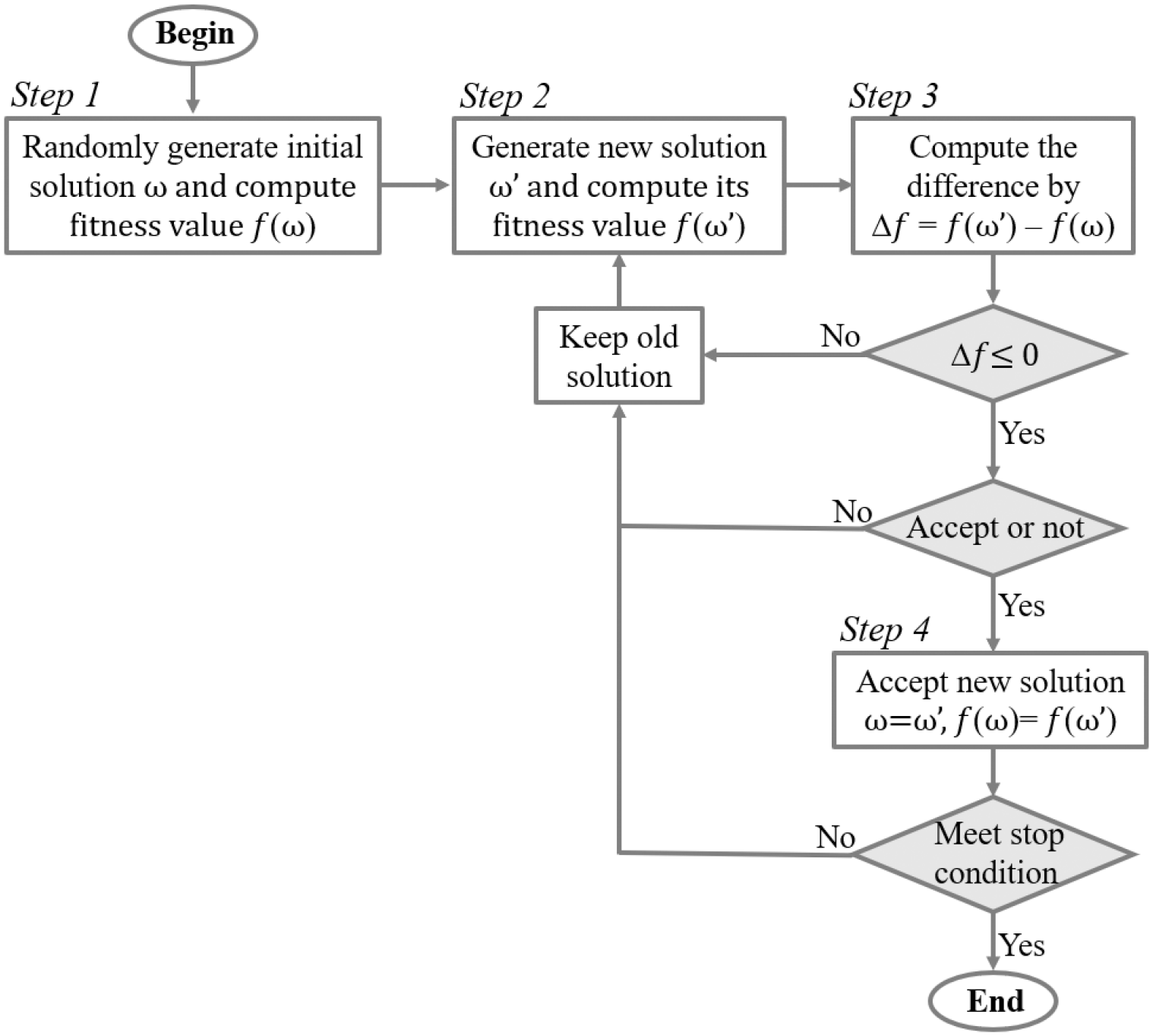
Workflow of spatial simulated annealing.
The optimization follows an iterative process where stations are added incrementally into the study; and locations are selected based on heuristic attempts to minimize the objective function. When adding new stations, the placement area is limited to a square region within the study area. This is done to reduce computational complexity and algorithm runtime. The number of RWIS stations to be located in this square region is arbitrarily limited to 10, which is equal to the existing number of RWIS stations in the square region. For the optimization process, two top criteria are implemented. If the number of iterations exceeds 100,000, the optimization process will stop. And if no improvements are made in the objective function after 200 iterations, the algorithm is set to automatically stop ( 7 ).
Case Study—Iowa, United States
Study Area and RWIS Network
The study area is in the state of Iowa, U.S.A. Iowa is generally a flatland area consisting of rolling plain lands and flat prairies. The altitude of this state is 146 m to 509 m ( 35 ). The total count of RWIS stations for Iowa is 88. The study period selected for this analysis includes a shoulder season month (October 2016) and a mid-winter month (January 2017) to best capture challenging winter driving conditions. Distribution of RWIS stations for the study area is presented in Figure 4. A randomly generated 10,000 km2 region within the study area is used as the experimental boundary for location optimization, presented as the red box below, in which there are 10 RWIS stations.
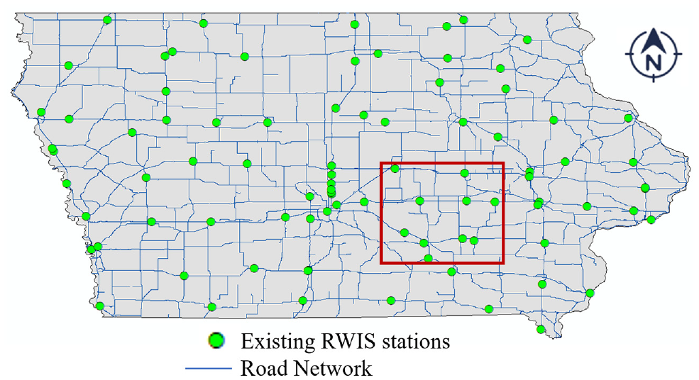
Distribution of road weather information system (RWIS) stations for Iowa.
Data Description and Quality Diagnostics
RWIS data for Iowa was downloaded from Iowa State University website (http://mesonet.agron.iastate.edu/RWIS/) as an Excel file. Measurements from a typical RWIS station include, but are not limited to AT, RST, DPT, visibility, wind speed, and road surface conditions. RWIS measurements were collected every 15 to 20 min, totaling 1488 h of data to be used in this study. As discussed previously (Figure 1), these data were processed to remove “noise” via four steps: (a) data completeness test to identify missing data, (b) reasonable range test to find erroneous data, (c) comparison with neighboring observations, and (d) detrending processed data with respect to time using GAM.
Statistical analysis was then performed using descriptive statistics of the processed data and correlation analysis among weather parameters. Descriptive statistics of AT, RST and DPT are presented in Table 1. On closer inspection of Table 1, it was revealed that there was relatively less variation in monthly temperatures in the mid-winter month than in the shoulder month for AT and RST, whereas DPT showed the opposite trend. AT varied from −6°C to 33°C over the month of October 2016, while the RST and DPT varied from −1°C to 41°C and from −8°C to 24°C, respectively. For the month of January 2017, temperature varied from −27°C to 20°C. Figure 5 shows the maximum, minimum, average, and standard deviation of weather data for the study area.
Descriptive Statistics of AT, RST, and DPT for the Study Area
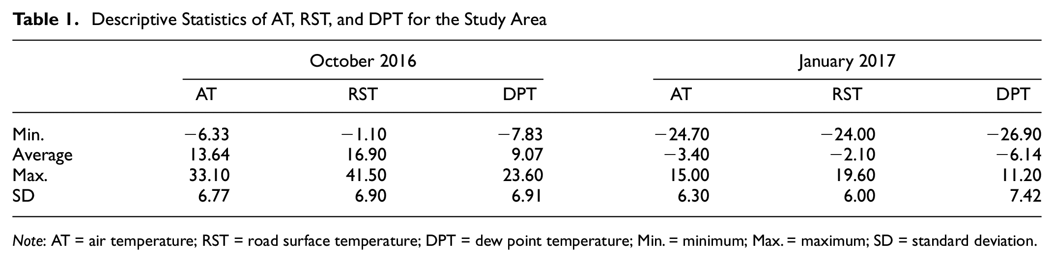
Note: AT = air temperature; RST = road surface temperature; DPT = dew point temperature; Min. = minimum; Max. = maximum; SD = standard deviation.
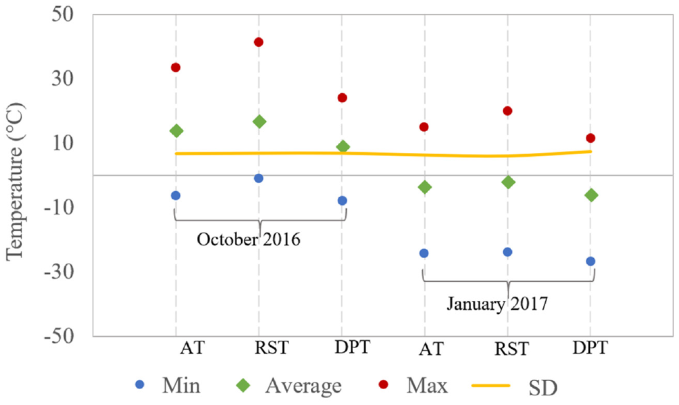
Plot of variation found in AT, RST, and DPT over the shoulder and winter months.
Correlation analysis was conducted among the weather variables to find how strongly two variables were correlated to each other using values between −1 and +1. A correlation coefficient of positive 1 indicates an ideal positive correlation, whereas a correlation coefficient of negative 1 indicates an ideal negative correlation. A correlation coefficient near zero indicates no correlation at all ( 36 ). Correlation analysis in this study was performed using the Analysis ToolPak in Excel. For each month, 10 RWIS stations were selected randomly, and the correlation coefficient values were generated between each pair of weather variables. These 10 values were then averaged to determine the resultant correlation coefficient. Table 2 shows the results from this analysis for October 2016 and January 2017.
Correlation Coefficient for AT, RST, and DPT for Study Periods
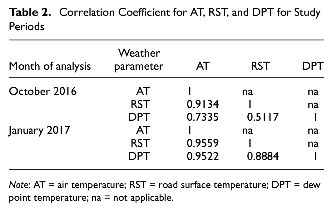
Note: AT = air temperature; RST = road surface temperature; DPT = dew point temperature; na = not applicable.
According to Table 2, the weather variables were more correlated during the mid-winter month than the shoulder month. Correlation between AT and RST was higher than for any other variable pairs, having a correlation value of over 0.9 in both study months. In contrast, the lowest level of correlation was observed between RST and DPT, thereby further attesting to the need for taking into consideration the distinctive road weather characteristics later in the location optimization phase. Figure 6 presents a plot comparing the correlation coefficient among AT, RST, and DPT of Iowa, and clearly shows that the three variables considered have different degrees of similarities over different months.
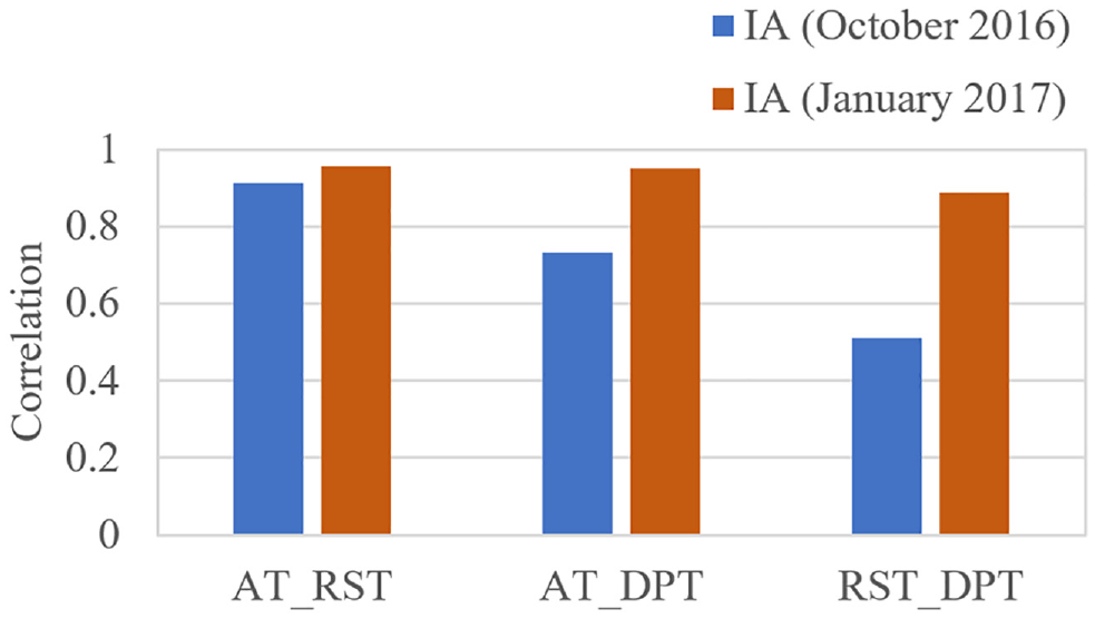
Correlation coefficients comparison of multiple weather variables.
Spatiotemporal Semivariogram Modeling
As evidenced in the previous section, correlation coefficients varied from one variable to another, and over different months. Spatiotemporal semivariogram modeling was subsequently conducted to gain a deeper understanding of their spatial and temporal variability, and to use as input to the location optimization model. For this purpose, RWIS data for those two select months were further processed and aggregated using 1 h interval for the time domain. A space–time matrix was then formulated as an input for the spatiotemporal analysis. Separate analysis was conducted for each month and each weather parameter, that is, AT, RST, and DPT. According to previous studies, 30 or more sampling points are needed to construct a reliable semivariogram model ( 19 ), which we exceeded by employing 88 stations from a robust RWIS network. Semivariogram modeling was performed using the R statistical package—version 3.2.5 ( 37 , 38 ). Table 3 represents the spatial, temporal, and joint semivariogram parameters, respectively.
Spatiotemporal Semivariogram Analysis Result
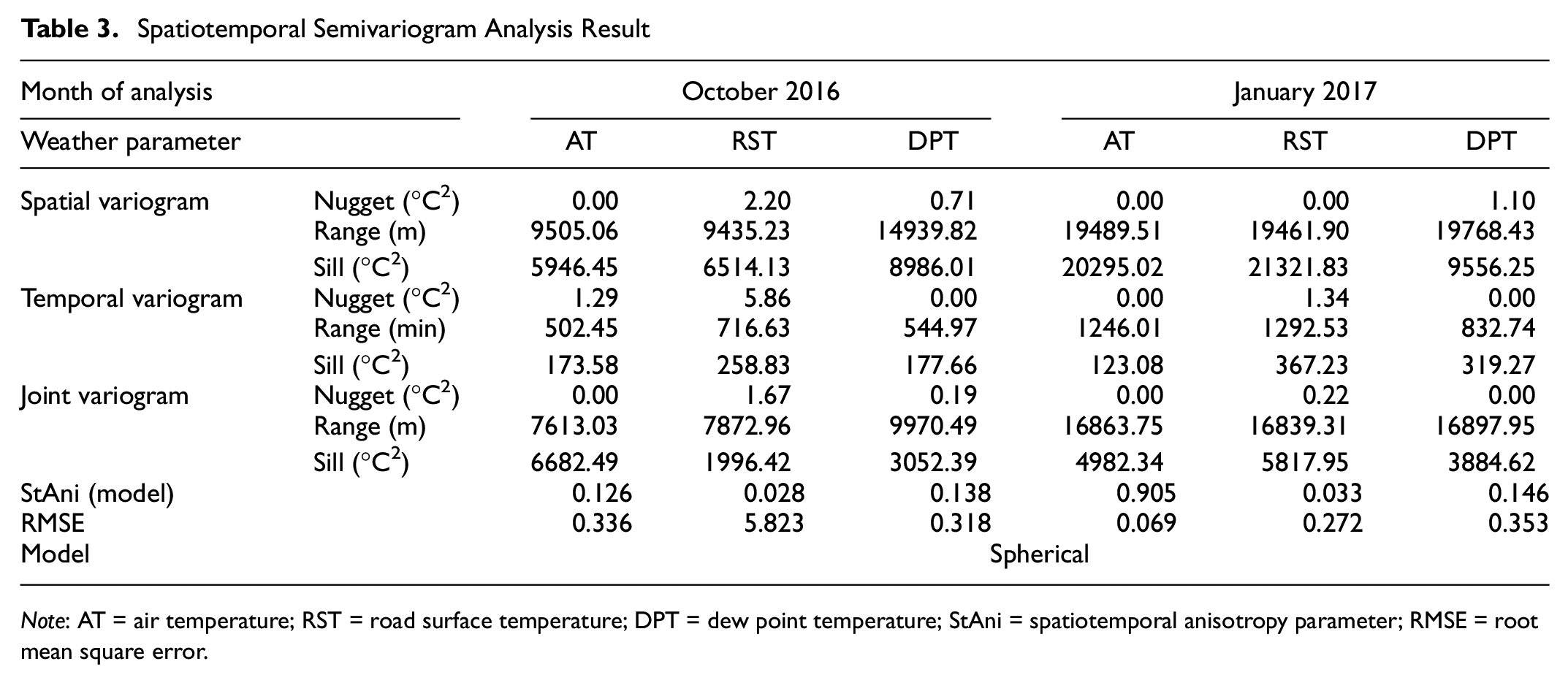
Note: AT = air temperature; RST = road surface temperature; DPT = dew point temperature; StAni = spatiotemporal anisotropy parameter; RMSE = root mean square error.
According to Table 3, higher spatial ranges were obtained for the mid-winter month than for the shoulder month. The spatial range is close to 20 km for all weather variables in January 2017, and a 10–15 km spatial range was obtained for October 2016. The temporal range was found to be 8.5–12 h for the shoulder month, and 14–21.5 h for the mid-winter month. Such findings make intuitive sense since road weather and surface conditions tend to change more abruptly during shoulder months than they do during mid-winter months when the variability of weather is relatively low ( 39 ). To consider these unique characteristics and implement them in the optimization phase, spatial and temporal semivariograms were combined using spatiotemporal anisotropy to estimate the joint semivariogram. The resultant joint semivariogram parameters are presented in Table 3 with the associated StAni and RMSE. Spatiotemporal range for January 2017 was found to be 17 km for all three weather variables, and 7.5–10 km for October 2016. It can be seen that the seasonal trend is well captured in the joint semivariogram parameters where a longer range was generated for the mid-winter month than for the shoulder month. In addition, the spatiotemporal range was found to be identical for the month of January, indicative of high correlation among three weather variables, whereas different degrees of correlations were observed for the month of October, possibly because of the presence of highly variable weather patterns. Based on the recorded results, the parameters of the joint semivariogram are used for RWIS location optimization.
Effect of Road Weather Variables on Optimal RWIS Locations
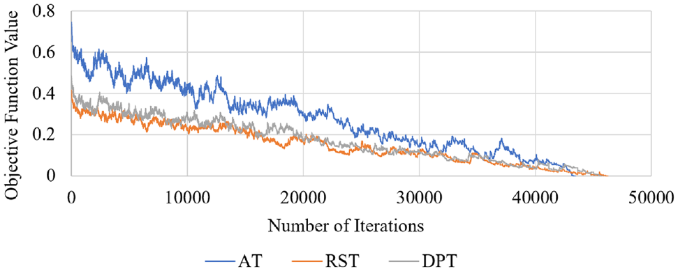
Optimal RWIS locations were determined by relying on spatiotemporal semivariogram analysis results that were obtained in the previous section. To quantitively appreciate the effect each road weather variable has on the resulting RWIS locations, the optimization was performed separately for each set of weather variables and month of data using the R statistical package—version 3.2.5 ( 37 , 38 ). To reduce the computational complexity associated with the location optimization process and shorten the algorithm runtime, a randomly selected square region (100 × 100 km) within the study area was used as the experimental boundary for location optimization. A 5 × 5 km prediction grid was generated along the square area in ArcGIS to create the candidate sites for RWIS station placement. The computer used to run the optimization was equipped with a 3.60 GHz CPU and 16 GB memory. An initial seed value was used for the optimization process to generate comparable results. The main goal of this location optimization is to prove the hypothesis that location solutions generated by individual weather variables may not lead to the same results, therefore revealing the need for generating multi-criteria location allocation optimization. The objective function value for each of the three sets of optimizations is plotted in Figure 7, a and b, for October 2016 and January 2017, respectively. The decreasing trend of the objective function value with respect to number of iterations demonstrates the superiority of the SSA algorithm implemented and its ability to achieve convergence near the 35,000th iteration. The average algorithm running time for generating each solution set was approximately 5 to 8 h.
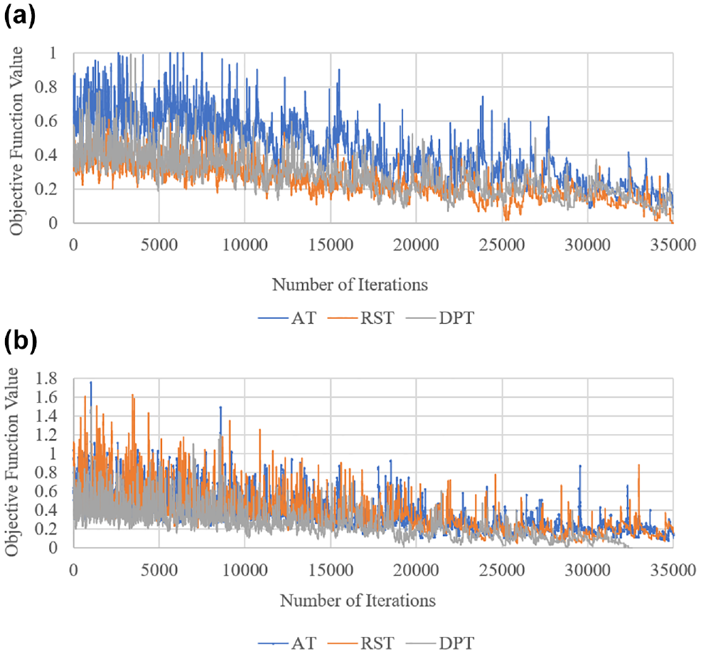
Plot of objective function with respect to number of iterations for three sets of road weather information system (RWIS) location optimization: (a) October 2016 and (b) January 2017.
As a result, the RWIS network optimization output under different weather variables is presented in Figure 8, a and b, for October 2016 and January 2017, respectively. A 10 km buffer was created around the stations arbitrarily to help better recognize the distribution of stations within the rectangle study area. It is evident that the RWIS location solution is substantially different depending on the variable of interest and over the month of analysis. These findings reveal that the spatiotemporal autocorrelations of the three weather variables have strong effect on generating optimal RWIS locations, and that there is a resurgent need to consider these effects collectively in the optimization framework so that locations selected are most representative of their uniquely different spatiotemporal characteristics.
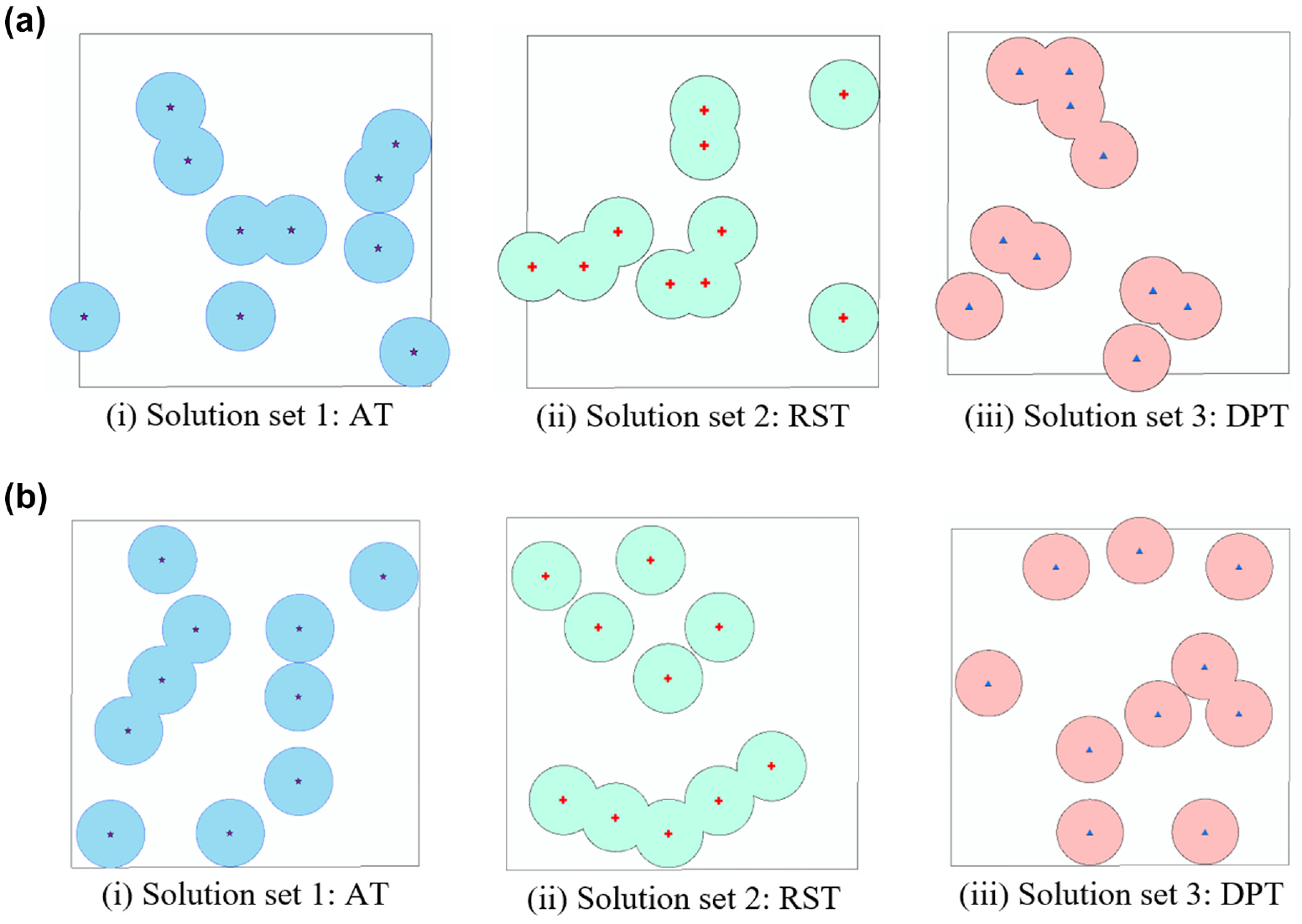
Spatial distribution of optimized road weather information system (RWIS) locations with respect to three variables: (a) October 2016 and (b) January 2017.
Spatial Similarity Analysis
It is obvious from the location allocation output (Figure 8) that the optimized location solutions are visually different from one another. To quantitatively evaluate the closeness of the optimal RWIS station distributions, a spatial similarity index was developed. For this, a sensitivity analysis was performed to objectively measure the similarity of optimal locations using ArcGIS ( 40 ). Initially, buffer polygons were created around the stations up to a maximum of 20 km in linear units. To perform this analysis, 10 sets of buffer polygons were created for each solution set, which totals up to 60 sets of buffer polygons. The intersecting areas were then determined for each pair of solution sets, each linear unit combination, and each month of analysis. The percentage of intersecting area with respect to the study area represents the spatial similarity index; the higher the percentage of intersected area, the more similar the solution sets. Figure 9 presents the results from this analysis.
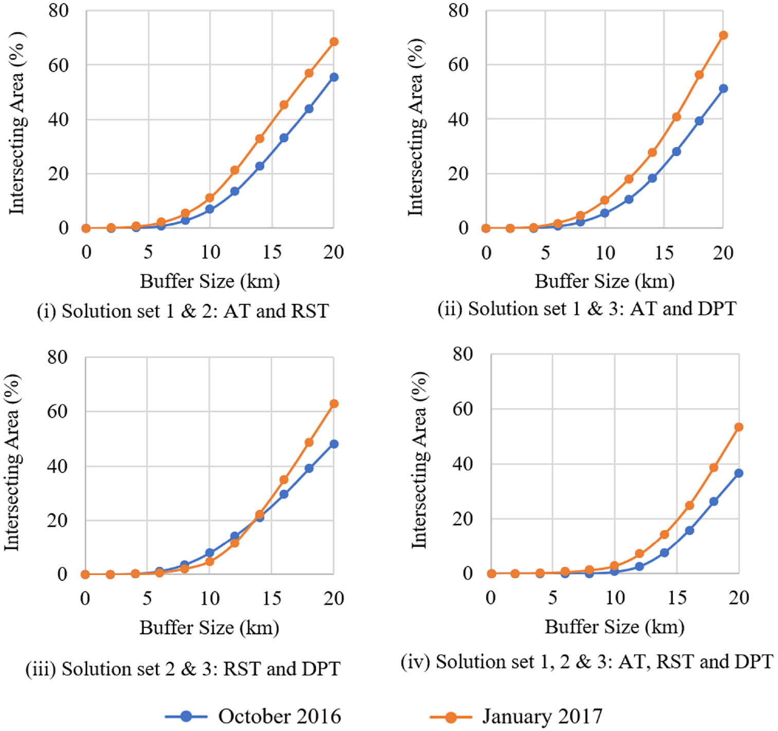
Similarity among optimal road weather information system (RWIS) station placements.
According to Figure 9, the percentage of intersecting area with respect to different buffer sizes follows an exponential function. It is clear from the figure that buffer size does not affect the results significantly. In most cases, location solutions generated using the mid-winter month (January 2017) data set have been found to be closer than those of the shoulder-month (October 2016) data set. The reason behind this outcome is that the daily fluctuation in weather data is greater during shoulder months than during mid-winter months, which generates relatively higher spatiotemporal autocorrelation of weather data for January than for October. For a specific buffer size, percentage of intersecting area between AT and RST solution sets was found to be the highest, followed by, in decreasing order, AT and DPT solution sets, RST and DPT solution sets, and AT, RST, and DPT solution sets. This phenomenon is quite similar to the correlation analysis results among the weather variables, where the correlation between AT and RST was the highest among all, followed by AT and DPT, and RST and DPT. The findings of this analysis indicate that spatial similarity of location solutions can be examined by creating buffer polygons regardless of the size implemented.
RWIS Location Allocation for the Entire Iowa State
In the previous section, it was confirmed using the hypothetical square region that the generated locations were dependent on weather variables. Based on this finding, the proposed location optimization method was expanded to cover the entire Iowa state. To achieve a comparable result to that for the existing RWIS locations, a constrained optimization was performed with respect to the road network using a shoulder-month data set of weather variables. Although the existing number of RWIS stations is 88, the total number of all new station has been set to 61 for the location optimization. The number 61 was chosen based on our previous study on optimal RWIS density guidelines ( 28 ), where the number of RWIS stations per unit area was generated given the topographic variation and weather severity of regions. In computational efficiency, the average running time for each set of optimization algorithms was approximately 78 h. Figure 10 represents the plot of the objective function value as a function of iteration; and Figure 11 shows existing and optimized RWIS locations with multiple weather variables. The spatial distribution of location solutions proves the previously generated hypothesis. It is evident that the optimal locations are different and largely depend on the underlaying spatiotemporal autocorrelation structure considered during the optimization process. The spatial similarity analysis was also conducted to objectively assess the difference between three solution sets generated and suggested that the spatial correlation between RST and DPT was lower than that of AT and RST, which is consistent with our hypothetical test results. These findings, undoubtedly, provide a stepping stone to the development of a multi-objective RWIS location allocation model by considering the varying degrees of representativeness of multiple weather variables.
Plot of objective function with respect to number of iterations for location optimization of Iowa.
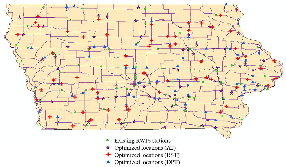
Existing and optimized RWIS locations of Iowa generated with three variables for October 2016.
Conclusion and Recommendations
This study aimed at developing an advanced location optimization model by using spatiotemporal semivariogram parameters combining both spatial and temporal effects of three key RWIS variables—AT, RST, and DPT. In the proposed method, a joint spatiotemporal semivariogram model was generated using three RWIS measurements; and the parameters of the model were used for determining optimal locations for RWIS stations. The location allocation problem was solved using a popular mathematical programming approach—an SSA algorithm that has been proven effective in and has gained recognition for RWIS location optimization problems. The methodological framework developed here builds on our previous effort by integrating the temporal domain in the location allocation problem. Additionally, RWIS data for multiple weather variables was used to generate three sets of optimal location solutions. The similarity among the generated location solutions was also quantified in this study using a spatial similarity index. The key findings of this research are listed below:
An advanced RWIS location allocation model was developed based on the premise that monitoring capabilities can be increased by minimizing the spatially averaged kriging variance in both space and time. The framework developed represents the first in the existing literature that attempts to determine optimal regional RWIS sampling design by taking into account both spatial and temporal attributes of multiple road weather variables.
This study investigated and confirmed that the location solutions generated using AT, RST, and DPT were significantly different from one another. Their closeness was further quantified and objectively validated using a spatial similarity index.
RWIS measurements of AT, RST, and DPT were processed and analyzed, and their correlations quantified, revealing that variables were more correlated with each other during mid-winter months than during shoulder months. Most notably, similarity between AT and RST was found to be significantly high.
The effective coverage of RWIS measurements was determined by analyzing multiple critical weather variables. Comparatively, a higher spatial and temporal continuity range of autocorrelation was observed for mid-winter months than for shoulder months. The spatiotemporal continuity range (from the joint semivariogram model) was determined to be 17 km for the mid-winter month, and 7.5–10 km for the shoulder month.
Recommendations for further research are given below:
This study covered a flatland region as the study area. Therefore, more case studies including wider regions can be examined for better understanding of the effect of spatiotemporal structure on RWIS location optimization.
The study period of this research was limited to 2 months: October 2016 and January 2017. Lengthening the study period can potentially improve the level of confidence in the output.
Three different weather variables were used in this analysis: AT, RST, and DPT. Thus, other RWIS measured data, that is, subsurface temperature, road surface conditions, and so forth could be included in the analysis to strengthen the output.
Microclimatic factors could be considered by combining RWIS data with other road weather and surface data extracted from entities such as automated surface observing system (ASOS) and airport weather observation system (AWOS). The combined spatially rich data set allows the RWIS location optimization algorithm to consider both the local and regional weather characteristics in the regions of interest.
Finally, a framework for a multi-criteria location optimization model should be established incorporating the joint semivariograms generated from weather variables.
Footnotes
Acknowledgements
The authors would like to thank Iowa DOT for providing the data necessary to complete this research.
Author Contributions
The authors confirm contribution to the paper as follows: study conception and design: S. Biswas, T. J. Kwon; data collection: S. Biswas; analysis and interpretation of results: S. Biswas, T. J. Kwon; draft manuscript preparation: S. Biswas, T. J. Kwon. All authors reviewed the results and approved the manuscript.
Declaration of Conflicting Interests
The author(s) declared no potential conflicts of interest with respect to the research, authorship, and/or publication of this article.
Funding
The author(s) disclosed receipt of the following financial support for the research, authorship, and/or publication of this article: This research is funded by Natural Sciences and Engineering Research Council (NSERC).