Procurement Benchmarks for Major Transportation Projects

Abstract

The U.S. transportation industry has long called for a schedule and cost benchmark tool to assist project sponsors with developing project delivery plans benchmarked in reference to similar past projects across the nation. Such a benchmark tool has recently been developed in response to the industry demand and a mandate of the Fixing America’s Surface Transportation Act. The tool capitalized on the Information Source for Major Projects database, which adopted standard processes and uniform terminology for documenting critical milestones throughout the project lifecycle. Based on 137 major transportation projects, the benchmark model produces schedule benchmarks on environmental study, procurement, and implementation processes. Also, the benchmark tool recommends a cost benchmark based on the Federal Highway Administration’s standard. Users have the flexibility to define a benchmark level and a suite of project features including type, size, class of action required under the National Environmental Policy Act, and delivery method such as design-bid-build, design-build or public–private partnerships. Benchmark level is the percentage of projects that outperform the other projects with the same selected features. The tool promises immense potential for milestone planning and can provide insightful expectation of project milestones in support of delivery method selection. Included in the tool are benchmark charts, a handy reference from which schedule benchmarks can be read. This paper demonstrates the use of the tool in a case example.

Keywords

policy and organization executive management issues economics revenue and finance public private partnership

Introduction

The United States is in dire need of a procurement performance benchmark tool on the national level to facilitate the planning of project development. One of the national goals of the federal-aid highway programs specified in 23 U.S.C. § 150 is to reduce project delivery delays and accelerate project completion. To ensure accountable expenditure of federal assistance, Title IX of the Fixing America’s Surface Transportation (FAST) Act (49 U.S.C. § 116) mandated the Build America Bureau to establish procurement benchmarks for different delivery methods as appropriate. The benchmarks, using a uniform method for measuring cost and schedule performance, will show maximum thresholds for acceptable project cost increases and delays. Besides the requirement by law, lending agencies are also concerned about the project delivery schedule and the overall cost. For example, in the Elizabeth River Tunnels project, the trustee of the $664 million private activity bond (PAB) required the borrowers to furnish monthly progress reports containing a description of any material change orders and a summary of the schedule to achieve substantial completion ( 1 ). Additionally, transportation agencies can compare their projects with similar major projects, see where improvement can be made to control cost and schedule, and plan accordingly.

The primary challenge associated with developing such a benchmark tool is data availability and quality. Project data on environmental studies and procurement are dispersed and, before the development of this tool, there was no central place where reliable data could be obtained. Unique project features create another type of challenge. A project could have multiple segments/phases within which multiple contracts could exist. There are numerous variations from a standard project procurement process which make cross-project comparison extremely difficult if not impossible. For example, a public–private partnership (P3) project could be developed from an unsolicited proposal; there could be an interim agreement before a comprehensive agreement was signed ( 2 ); and there could be multiple agreements signed for the overall development framework and phased development of specific facilities (3 –5). The challenges also stem from different delivery methods and contracting mechanisms. In design-bid-build (DBB), the design is completed first and then the construction contract is let, whereas in design-build (DB) and P3, the design and construction are design-builder’s or developer’s responsibilities, and design is usually completed after awarding the contract. In a construction manager at risk (CMAR) project, although design activities and construction management procurement proceed concurrently, the construction contract with a guaranteed maximum price (GMP) will not be let until the design for that part is completed. Additionally, there is resistance from state and local transportation agencies to evaluating the performance of their projects. It takes significant effort to collect relevant data from public sources to have a sufficiently large and high-quality dataset for making this benchmark tool a reality.

To a great extent, these challenges were addressed by the Information Source for Major Projects (ISMP), an open-access, comprehensive database for U.S. major transportation projects receiving federal funding. Sponsored by the Federal Highway Administration (FHWA), the database contains detailed project life-cycle data from cost and funding to milestones in the environmental study, procurement, and project implementation stages. The database adopted standard processes and uniform terminology so that cross-agency comparisons remain valid. A case in point is that the Elizabeth River Tunnels project had an interim agreement signed before the comprehensive agreement, which was not typical for P3 procurement; the database treated the signing date of the interim agreement as the contract award date and the signing date of the comprehensive agreement as the commercial close date. Moreover, the data quality was ensured through reliance on primary documents and verification by the project sponsors. Last, the data cover common delivery methods, allowing for benchmarks for different delivery methods in the benchmark tool.

Capitalizing on ISMP, the authors developed the Procurement Performance Benchmark tool in collaboration with the Build America Bureau to fulfill the FAST Act mandate. At a user-specified benchmark level, that is, percentage of projects that outperform their peers, the tool gives schedule benchmarks in the environmental study, procurement, and implementation phases and cost benchmark at substantial completion, while allowing for selection of projects by project type, project size, class of action (for the environmental study process), and delivery method. It is the first tool with the said functions. The following sections will review the current practice, explain the different processes for which the tool presents information, discuss the methodology, and demonstrate the user interface and the application of the tool and the derived benchmark charts in a case example.

State of Practice

There are other options to check the schedule performance of environmental review and permitting processes for transportation projects. One option is the Federal Infrastructure Permitting Dashboard, which was mandated by Title XLI of the FAST Act (FAST-41 or 42 U.S.C. § 4370m et seq.) and managed by the Federal Permitting Improvement Steering Council (FPISC). The statute 42 U.S.C. § 4370m-1 requires FPISC to recommend, at least once every two years, performance schedules for environmental reviews and authorizations based on the average time from when the project is entered in the dashboard to the issuance of a decision document. Regrettably, the performance schedules in the Fiscal Year 2019 update did not include transportation projects because of data limitation, nor did it specify the project type, project size, or delivery method ( 6 ). The dashboard also features the Infrastructure Permitting Performance Accountability Scorecard, which was required by executive order (EO) 13807 and implemented through the Office of Management and Budget’s Performance Accountability System. The quarterly scorecard tracked compliance with One Federal Decision and related provisions of EO 13807 for major infrastructure projects as defined in Section 3(e) of EO 13807, and evaluated agency performance, which was linked with budget formulation ( 7 ). However, only nine major infrastructure projects led by U.S. Department of Transportation (U.S. DOT) and subject to National Environmental Policy Act (NEPA) documentation have been enforced by EO 13807 since it was issued on August 15, 2017 ( 8 ). The EO was revoked on January 21, 2021, therefore no new scorecards will be published.

The Council on Environmental Quality (CEQ), which advises NEPA implementation, publishes the Environmental Impact Statement (EIS) Timelines, which tracks the schedule performance between milestones of the EIS process for all federal agencies implementing NEPA. The June 2020 update of the timelines report covered 1,276 EISs for which a notice of availability of the final EIS was published between January 1, 2010 and December 31, 2018, and a record of decision (ROD) was issued by June 18, 2019 ( 9 ). However, the data did not contain the project type, project size, or delivery method, limiting the extent to which project sponsors can relate the reported statistics to their own projects.

Unlike the permitting dashboard and the EIS timelines, which are publicly accessible, the Environmental Document Tracking System (EDTS) is an internal database of FHWA for the agency to track NEPA project progress and measure success. In 2013, EDTS merged with the Project and Program Action Information System to become one system ( 10 ). The information is used for regular reports to CEQ as well as FHWA and U.S. DOT leadership ( 11 ).

As for performance monitoring of the project procurement and implementation processes, state departments of transportation use their own performance management systems ( 12 ). For example, the Virginia Department of Transportation uses its project dashboard to check the time and budget statuses of the project development and delivery. Data for the project dashboard include budget and cost, on-time and on-budget statuses and the reasons thereof, and the start and end dates of local agreement, scoping, public engagement, utility relocation, right-of-way acquisition, permitting, bid solicitation, contract award, and so forth, for both the planned and actual dates. Although DB project activities are coded, the dashboard does not support grouping by delivery method ( 13 ). Additionally, the Texas Department of Transportation has a performance dashboard that tracks the percentages of highway contracts completed on time and on budget. However, alternative delivery type projects such as DB and P3 projects are not included ( 14 ).

The delivery method is a key driver of project time and cost performance. Sullivan et al. ( 15 ) compared 30 studies, representing 4,623 projects, on the impact of delivery method on time and cost performance to conclude that CMAR and DB are more effective in controlling schedule variations than DBB by weighted average schedule growth. They also found that DB shows better cost performance than CMAR and DBB. Other studies observed that P3 exhibits superior time and cost performance than DBB ( 16 ) and is associated with a smaller cost change than DB ( 17 ). However, these results were valid as far as the construction activities were concerned. Few studies considered the procurement process or used the total capital cost, which includes, besides construction, elements such as preliminary engineering, right of way, utilities, risks, and finance charge. Another driver of project performance is project type. Choi et al. ( 18 ) demonstrated different patterns of schedule performance of contracting strategies among three project types: roadway resurfacing, reconstruction and rehabilitation projects, bridge projects, and capacity-added projects. Flyvbjerg et al. ( 19 ) found that project type matters for cost escalation. Project size also drives project time and cost performance. Large infrastructure projects often experience time and cost overruns ( 20 ). Nguyen et al. ( 21 ) surveyed 79 transportation projects to find that scope complexity, partially defined by project size related to capital cost, is positively correlated with schedule growth. Gkritza and Labi ( 22 ) examined 1,957 highway contracts in Indiana and showed that contracts of larger size or longer duration tend to increase cost overruns. In sum, delivery method, project type, and project size are important considerations in project performance evaluation. However, the preceding tools did not consider all three factors. Moreover, the available tools are primarily used for performance evaluation rather than planning. State and other public sponsor agencies desire a planning tool to estimate reasonable project delivery timelines and costs.

Procurement Process and Milestones

Environmental Study Process

NEPA (23 U.S.C. § 4321 et seq.) is a procedural statute that “declares a broad national commitment to protecting and promoting environmental quality,” and imposes “action-forcing” procedures on federal agencies undertaking major federal actions to “take a hard look at environmental consequences” and “provide for broad dissemination of relevant environmental information” ( 23 ). It is the basic national charter for protection of the environment. Coordinating federal environmental efforts under NEPA is CEQ, which issues general regulations and guidance for implementing NEPA. CEQ regulations (40 CFR §§ 1500–1508) and 23 CFR § 771, highway-specific implementing regulations issued by U.S. DOT, allow three classes of actions, that is, environmental impact statement (EIS), environmental assessment (EA), and categorical exclusion (CE), each requiring different documentation. Before a class of action is determined, early coordination including the scoping process is typically conducted to involve the coordinating agencies and the public and identify the key issues to be addressed. If it is determined that the proposed action requires an EIS, the lead agency shall publish in the Federal Register a notice of intent (NOI) which “will establish a 30-day period for comments on the purpose and need, alternatives, and the scope of the NEPA analysis” (23 CFR § 771.111). An EIS is required when the proposed action will have a significant impact on the environment, and NOI for the purposes of this benchmark tool marks the start of the EIS process. Typically following the NOI, a draft EIS (DEIS), which describes all reasonable alternatives including the no-build alternative, is prepared. Although a preferred alternative is not required at this stage, the DEIS must state any official positions taken on any alternatives. After the DEIS is approved by the lead agency (usually the FHWA division office if FHWA is the lead agency) and a notice of availability is published with the Federal Register, the public is allowed a period between 45 and 60 days for comments on the DEIS (23 CFR § 771.113[k]). During this period, public hearings for the purpose of disseminating DEIS information and collecting comments are usually held. Responses to all substantive comments must be included in the final EIS (FEIS), along with a note of changes from DEIS in response to the comments. The FEIS must also identify a preferred alternative and the basis for the decision, and show compliance to the extent possible with all applicable environmental laws and executive orders ( 24 ). The decision document under the EIS processing option is the ROD. If the ROD is not combined with the FEIS, it may not be issued sooner than 30 days after the publication of FEIS or 90 days after the DEIS is circulated (23 CFR § 771.127[a]).

The second processing option under NEPA is EA. An EA is a concise public document that is prepared for actions in which the significance of the environmental impact is not clearly established. As soon as the decision to pursue an EA is made, FHWA (for FHWA undertakings) will send an intent of study (IOS) letter to the cooperating agencies notifying them of the study and soliciting their comments. The EA must be approved by FHWA before it is made available for public inspection and comments. The EA need not be circulated, but a notice of availability must be sent to the state clearinghouse for publication. The availability period is usually 30 days, during which a public hearing may or may not be required. If it is concluded that the project will have no significant impact on the quality of the environment, a finding of no significant impact (FONSI) is issued. The FONSI, which modifies the EA according to the comments received, is not required to be circulated, but the state clearinghouse must be notified of its availability ( 24 ).

The third processing option, CE, means a category of actions that do not individually or cumulatively have a significant effect on the environment. The CE process typically starts with a determination to be processed as CE and ends with a CE approval. If the proposed action is one of the project types listed in 23 CFR § 771.117(c), the project needs no further documentation for approval. For projects that fall under 23 CFR § 771.117(d), the project sponsor must submit documentation to establish that the project satisfies the specific conditions or criteria thereunder and that significant environmental effects will not result. With a programmatic agreement, FHWA can delegate the authority of CE determination and approval to state departments of transportation.

There are variations to the standard NEPA process. If FHWA determines that the environmental documentation is no longer valid, the project sponsor is required to furnish a reevaluation that documents any changes to the project concept or affected environment and recommends the validity of the environmental documentation. If the changes result in significant environmental impacts, then a supplemental EIS will be required (23 CFR § 771.130). If the ROD has already been issued, then a revised ROD will be issued to replace the original ROD. Additionally, tiering of EISs is not uncommon in transportation projects. The first tier EIS deals with broad issues such as general location, mode choice, and area wide air quality and land use implications of the major alternatives, whereas the second tier focuses on site-specific details on project impacts, costs, and mitigation measures (23 CFR § 771.111[g]).

Procurement and Implementation Process

For all delivery methods, substantial completion is considered the end of the project implementation process since the milestone marks the start of availability of the facility for its desired function and often the start of the availability payments and repayment of debts. Using substantial completion allows meaningful parallel comparisons between delivery methods. As for the link between project implementation and the NEPA process, any substantive project approvals (e.g., final design, right-of-way acquisition, purchase of materials, construction) must not be authorized before the NEPA decision document (i.e., ROD, FONSI, or CE) is issued. For DB and P3 projects, procurement and contract award can precede the conclusion of the NEPA process (23 CFR § 636.109). Therefore, the authors double-checked the data to make sure mistakes such as design start occurring before ROD issuance no longer remained.

For the procurement and implementation process, the benchmark model considers the differences among DBB, CMAR, DB, and P3. The DBB process proceeds in a linear fashion, starting with design start. The design must be finished before the invitation for bid (IFB) is issued. Bidders will submit bids in response to the IFB. Usually, the winner is selected on the lowest price basis. The contract is awarded after the owner negotiates and confirms with the apparent lowest bidder on the price and contract terms. Then the winning bidder will provide the performance and payment bonds and insurance proof, and the owner will get final approval for the contract to be executed.

For CMAR contracts, the design will be procured first. The procurement of construction management services will follow with the issuance of a request for qualifications (RFQ). Interested bidders will respond with a statement of qualifications, and the most qualified bidder will be selected. Sometimes a second step of selection involving a request for proposals (RFP) will be used. Proposals will be submitted, and a winner will be awarded a CMAR contract. The construction manager will assist the designer with design development and put together a guaranteed maximum price (GMP) package for the construction work. Usually, the construction manager will get the GMP contract. However, if the owner decides otherwise, the GMP contract will be publicly let.

DB and P3 processes are similar as they both start with a request for information (RFI) to solicit input on construction and the terms of the delivery method, although RFIs are more common in P3s. After receiving the letters of interest, the owner will issue an RFQ and allow those who submitted letters of interest to respond. Following receipt of the statement of qualifications, the owner will announce a shortlist of proposers who will later receive an RFP. Typically for P3 projects, before the issuance of the final RFP, several versions of draft RFP will be issued to clarify questions and concerns about issues such as financing and disadvantaged business enterprise requirements to develop the RFP further. After proposals in response to the final RFP were received and evaluated, there is typically a conditional award, followed by a negotiation of the price and terms to reach the final award. Like the other delivery methods, the winning bidder will provide the necessary certificates and the owner will get the required approvals. After this, both parties will sign the contract in what is called commercial close. At this stage, all permits should have been obtained, except when part of the deal is to have the P3 developer help secure a permit. The P3 developer is allowed to perform limited activities after commercial close pending financial close, which is when the parties will sign off on any financial instruments pledged to finance the project ( 25 ).

Atypical procurement processes are sometimes seen in P3 projects. One example is unsolicited proposals. After accepting an unsolicited conceptual proposal, the owner may begin conceptual discussion with the proposer and decide if the proposal will receive further consideration, as in the case of the Florida Department of Transportation ( 26 ). Then, the department will advertise for detailed proposals on the approved concept. Alternatively, as in the case of the Virginia Department of Transportation, the owner may invite competing conceptual proposals. On passing the deadline for accepting competing proposals, the owner will evaluate the conceptual proposals and determine whether to advance one of the proposals. If the decision is to advance the project, detailed proposals will be requested from the proposers. The detailed proposals will then be reviewed, and a winning bidder will be selected ( 27 ). Additionally, an interim agreement may be allowed before the comprehensive agreement. This could happen when the NEPA process is not yet complete and the owner wants the winning bidder to commence limited activities including project planning and development, advance right-of-way acquisition, and design and engineering ( 28 ). The third example is the combined use of a comprehensive development agreement and facility concession agreements. The comprehensive development agreement provides the overall framework for the development of one or more facilities, whereas the facility concession agreement pertains to the services rendered for an individual facility ( 29 ).

Procurement Performance Benchmark Model

The procurement performance benchmark model follows a data-driven approach and considers key project features for benchmark determination and milestone planning. The overall benchmark development is described in Figure 1 and detailed in the following sections.

Figure 1.

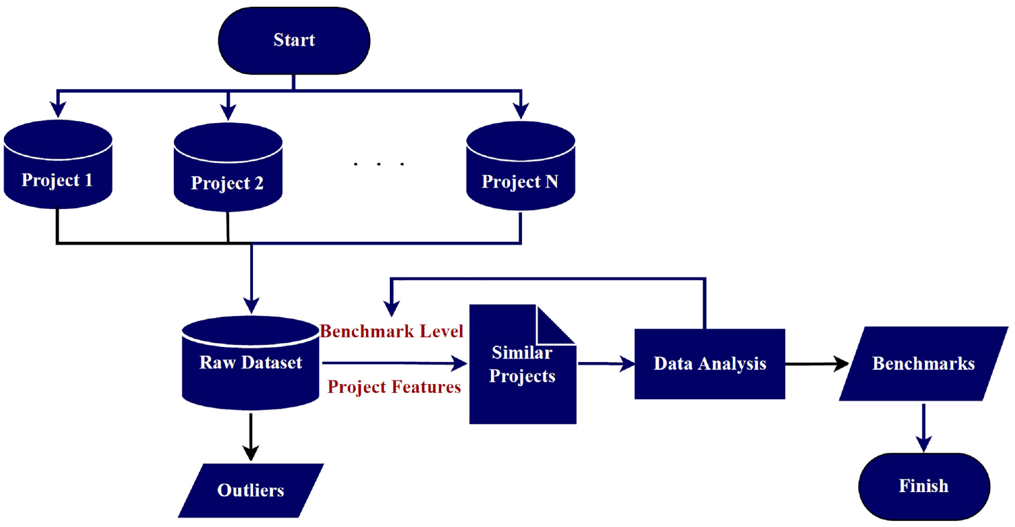
Procurement benchmark development flowchart.

Data Profile

ISMP served as the main source of project information in this study. Comprising 137 major transportation projects completed over the past 20 years in the U.S., the database covers a range of project types, project sizes, delivery methods, and locations to enable the development of a reliable performance benchmark tool. Several document sources were referenced to cross-validate the data. More credit is given to documents issued by the project sponsor or other official authorities. Figure 2 exhibits a descriptive summary of project features including type, size (million dollars), delivery method, and class of action.

Figure 2.

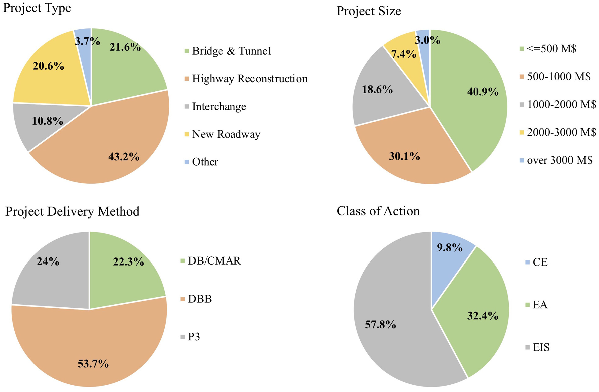
Descriptive statistics of project features.

Method

Benchmark Input

The benchmark level and project features need to be defined before calculating benchmark duration. Benchmark level is the percentage of similar projects that outperform their peers. The smaller the benchmark level, the shorter the benchmark durations. If the benchmark level is set at 70%, then 70% of similar projects completed the activity faster than the schedule defined by the 70% benchmark level. The second element of user input is to define which projects are going to be used for benchmark calculation and performance comparison. Users can make a selection based on project type, project size, class of action, delivery method, or any combination of these. The selection of these features is flexible and depends on the purpose of benchmarking. This flexibility is valuable for users to compare performance.

Benchmark Design

With the input variables of the benchmark model defined, this section illustrates the design of the benchmark process. The first step is to get the raw durations for each project in the tool. Each duration is calculated based on the milestone dates according to Table 1. Detailed calculations are demonstrated in pseudocode in the Appendix (Figure A1).

Table 1.

Raw Duration Calculation for Each Window

Duration (months)	Formula
COA determination to CE approval	$(CE Approval - COA Determination) / 30$
IOS to FONSI	$(FONSI Approval - IOS) / 30$
NOI to DEIS	$(DEIS Approval - NOI) / 30$
DEIS to FEIS	$(FEIS Approval - DEIS Approval) / 30$
FEIS to ROD	$(ROD - FEIS Approval) / 30$
Design start (DBB) to IFB issuance	$(IFB issuance - Design Start for DBB) / 30$
RFI issuance to RFQ issuance	$(RFQ Issuance - RFI Issuance) / 30$
RFQ issuance to RFP issuance	$(RFP Issuance - RFQ Issuance) / 30$
RFP issuance to commercial close	$(Commercial Close - RFP Issuance) / 30$
Commercial close to financial close	$(Financial Close - Commercial Close) / 30$
Commercial close to substantial completion	$(Substantial Completion - Commercial Close) / 30$

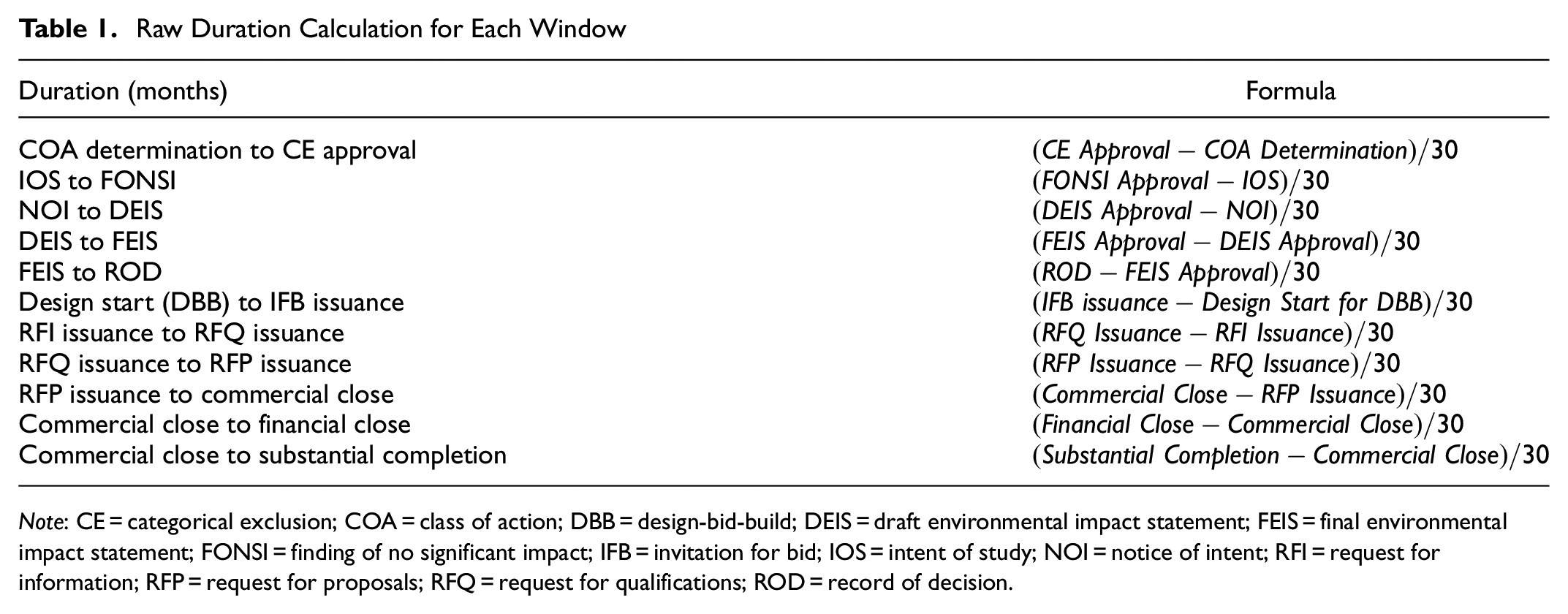
Note: CE = categorical exclusion; COA = class of action; DBB = design-bid-build; DEIS = draft environmental impact statement; FEIS = final environmental impact statement; FONSI = finding of no significant impact; IFB = invitation for bid; IOS = intent of study; NOI = notice of intent; RFI = request for information; RFP = request for proposals; RFQ = request for qualifications; ROD = record of decision.

A key assumption in the methodology is the probability distribution of the data points. Typically log-normal, beta, or gamma are used to represent construction durations statistically ( 30 ). The authors assumed that durations followed a log-normal distribution and tested the assumption. By definition, if durations follow a log-normal distribution, durations in the logarithm scale will follow a normal distribution. A standardized Q-Q (quantile-quantile) plot will compare the quantiles of empirically observed data points with the theoretical distribution. If the theoretical distribution and empirical observation are the same distribution, the points should fall along the 45-degree reference line. Figure 3 shows two examples of Q-Q plots, which demonstrate that log-normal distribution can be reasonably assumed.

Figure 3.

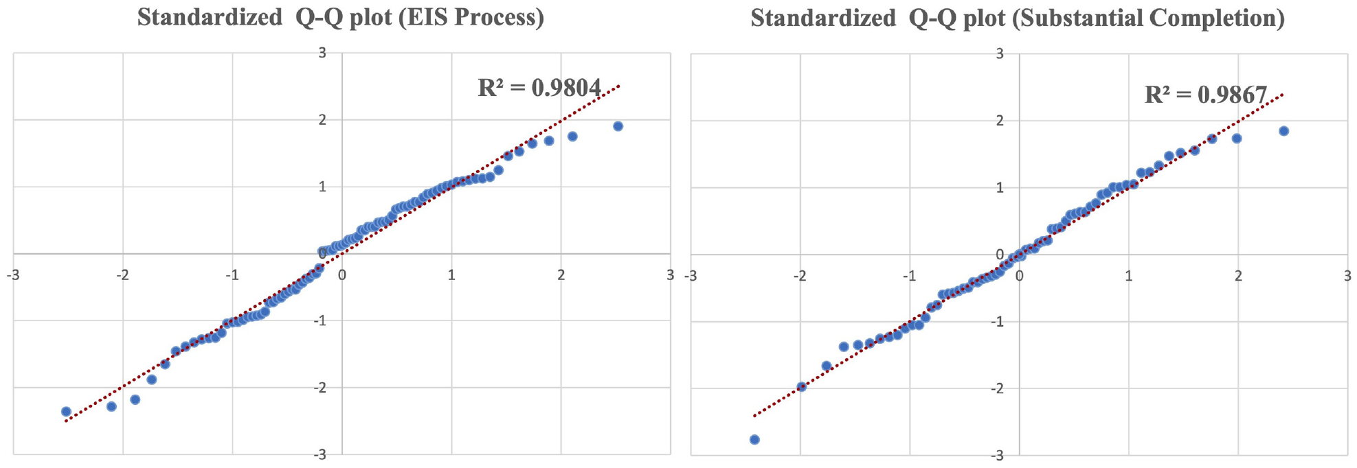
Distribution Q-Q plot checking.

The next step is to eliminate the outliers. The raw data are natural logs of the durations, and the outliers are assumed to lie two standard deviations outside of the mean of the raw data. Removing the outliers prepares the data points for benchmark calculation.

Benchmark Output

The final step is to calculate the benchmark duration output. Using the cleaned dataset, projects that satisfy the defined features are selected from the database. Using the inverse cumulative distribution function for log-normal, the benchmark duration will be calculated given the benchmark level and average and standard deviation of the selected projects.

Cost Benchmark

Calculation of the cost benchmark relies on the schedule benchmarks. The FHWA Major Projects Team allows for an annual cost increase of 2%. If cost growth exceeds 2%, the FHWA Division Office overseeing the major project must show efforts planned or spent to control cost growth ( 31 ). After a user enters a cost estimate, the model will assume the cost as-of date to be contract award/commercial close and apply the 2% threshold to determine the cost benchmark at substantial completion.

Interface

The Excel-based benchmark tool consists of several tabs. The dashboard tab presents the schedule benchmarks at the user-selected benchmark level (Figure 4). Users can customize the selection of projects based on project type, project size, class of action, and delivery method. This filtering function and the input of benchmark level are available in the left section of the dashboard sheet. The left middle section consists of bars showing duration benchmarks and diamonds showing milestone benchmarks. The environmental study durations are organized at the top, and the procurement and implementation processes are shown at the bottom. The right middle section contains pie charts showing the distributions of the selected projects based on project type, project size, class of action, and delivery method. On the very top of this sheet, the number of projects/contracts, average project size, and total project value of the selected projects are displayed. The right section of this sheet allows users to enter the information of a new project that they want to evaluate. The schedule performance of the new project will be plotted next to the benchmark bars to allow for a quick visual comparison. The 70% cost benchmark will be automatically calculated with the original cost estimate entered. The figure tab contains benchmark charts of various milestones for various benchmark levels, project size ranges, and delivery methods. Figure 5 shows example benchmark charts. The curves allow for planning of future milestones given the project size and delivery method. The selected projects and a descriptive analysis of their durations are shown in the data tab. The guide tab illustrates the layout and functionalities of the dashboard. Terms and abbreviations are explained in the definition tab.

Figure 4.

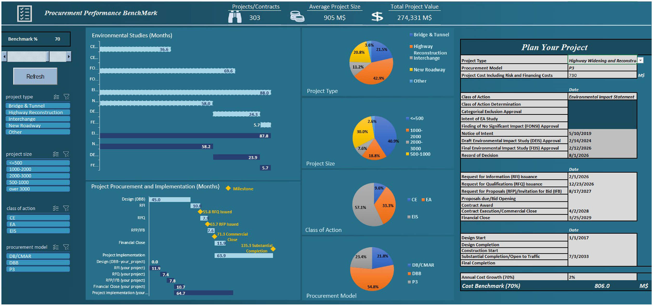
Dashboard tab layout.

Benchmark Charts

The benchmark charts as presented in Figure 5 serve as a handy reference for trends by benchmark level, project size, and delivery method. On the x-axis of each chart, the project size increases from less than or equal to $500 million to more than $3 billion; the y-axis shows duration in months. The EIS process refers to the duration from NOI to ROD. Commercial close in the charts measures the duration from design start to commercial close for DBB and the duration from RFI/RFQ issuance to commercial close for DB and P3. The substantial completion measurement is the sum of the commercial close measurement and the duration from commercial close to substantial completion. The authors made the following observations:

In DBB, the EIS process, commercial close, and substantial completion exhibit similar trends, whereas in DB and P3, the pattern of the EIS process appears different from the other two measurements.

In DB and P3, commercial close and substantial completion follow similar trends for projects of certain size ranges: $2 billion or smaller for DB and $3 billion or smaller for P3.

DB and P3 trends for the EIS process are comparable for projects worth between $500 million and $3 billion.

DB and P3 have similar trends and close duration values for commercial close in the less than or equal to $1 billion range and for substantial completion in the less than or equal to $2 billion range.

Figure 5.

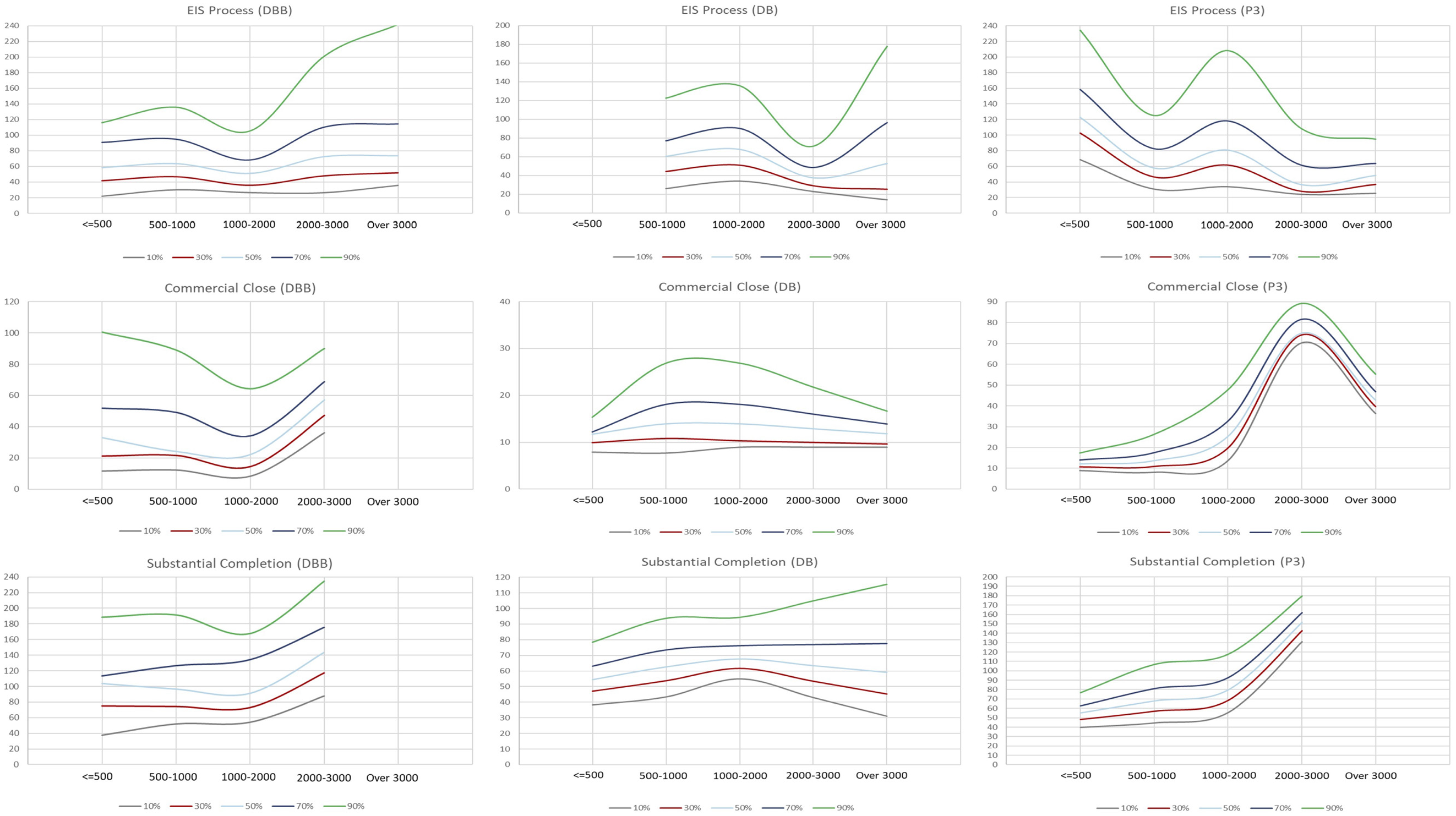
Benchmark charts.

Application

Case Study

The use of the benchmark tool will be demonstrated with a real case example, the Hunts Point Interstate Access Improvement Project. The project improves the access between the Hunts Point Peninsula, located in the South Bronx, New York, and Sheridan Boulevard and Bruckner Expressway (I-278) for 78,000 vehicles daily to and from the peninsula. The improved access will serve the Hunts Point Food Distribution Center (the largest of its kind in the nation), industrial and commercial businesses outside of the food distribution center, and residents in the northeast part of the peninsula. The $1.7 billion project addresses the concern over commercial trucks traversing the local streets. The project also addresses the geometric and operational deficiencies of the Bruckner/Sheridan Interchange, repairs the Bruckner Expressway viaduct and ramps, and replaces the westbound Bruckner Expressway truss bridge over Amtrak ( 32 ). The entire project is expected to bring 22,000 jobs. Programmed to receive $328 million federal funding, the project underwent an EIS process and will be completed in three phases. Phase 1 totals $598 million, and its $460 million DB contract was executed in October 2019. Construction began in December 2019. Phase 1 work includes replacing four bridges over Bronx River Avenue and Amtrak/CSX rail lines, improving the intersection of Bruckner Boulevard and Hunts Point Avenue, and creating more pedestrian and cycling spaces. Phase 2 rehabilitates 1.25 miles of Bruckner Expressway between 141st Street and Barretto Street and was also procured in DB. Signed in March 2021, the $518 million contract was expected to end in November 2023 ( 33 ). Phase 3 includes the demolition of the existing Hunts Point Avenue entrance ramp and the reconfiguration of the Bruckner-Sheridan Interchange. Estimated at $578 million, Phase 3 is being procured as a DB contract as of March 2022. Notice to proceed will be issued in November 2022 according to the RFQ.

Milestone Planning

The benchmark tool can assist with the planning of milestones and resources. Knowing the completed or target milestone dates of a project to be evaluated, a user first enters the information in the “Plan Your Project” section of the dashboard tab. Key milestones will be automatically calculated based on the selected project features and benchmark level, and the schedules will be plotted accordingly in the schedule bar section. The more control of the target dates the user has, the better they will be able to identify a comparable benchmark level for the new project. If a future activity takes substantially longer than the benchmark duration, the user can look for a realistic goal by reading off a value from an appropriate benchmark chart in the figure tab. The agency can subsequently make an acceleration plan reflecting the extent to which it can mobilize resources.

The Hunts Point project had a fast-tracked EIS process. The NOI was issued on May 22, 2017; the DEIS was approved on May 21, 2018; the FEIS/ROD was approved on April 9, 2019. The 22.9-month schedule places the project within the top 1% (benchmark duration of 23.8 months), thanks to the new requirements of EO 13807 ( 34 ). By comparison, the 50% and 70% benchmarks for similar projects (i.e., the selection of highway reconstruction, $1 billion to $2 billion, EIS, and DB) are 64.0 months and 80.8 months, respectively. The extraordinary performance was more about the now-rescinded two-year cap of the EIS process and less about the project features. So, it is not fitting to use 1% to plan for future milestones. The authors proceeded to look at the individual phases. The feature selections for both Phase 1 and Phase 2 were highway reconstruction, $500 million to $1 billion, EIS, and DB. For Phase 2, RFQ issuance to RFP issuance and RFP issuance to commercial close took 5.8 months and 8.0 months, which were on par with the 50% benchmarks of 5.8 months and 7.7 months, respectively. Using the end of 2023 as the substantial completion date (by contract stipulation), the duration from commercial close to substantial completion came out to be 34.4 months, about five months shorter than the 50% benchmark (39.3 months). Phase 1 RFQ and RFP processes were 7.4 months and 8.8 months in length. The total procurement duration (16.2 months) was close to the 98% benchmark (16.3 months). The authors compared the final RFP and the conformed RFP of Phase 1 to find out that the procurement schedule was delayed for one and a half months; the actual commercial close date was delayed for another one and a half months from the date in the conformed RFP. The actual 16.2-month procurement duration minus the three-month delay is 13.2 months, close to the 50% benchmark (13.5 months). The commercial close to substantial completion duration (36.3 months), assuming the substantial completion not-to-exceed date of September 30, 2022 is the current best estimate, was three months shorter than the 50% benchmark (39.3 months). Therefore, it is reasonable to surmise that the project is on a trajectory to hit the 50% mark if everything goes well. The 50% benchmark milestone for substantial completion is 52.8 months, close to the 52.5-month current plan of Phase 1 (sum of 7.4 months, 8.8 months, and 36.3 months). If using the benchmark chart, which only considers the project size and delivery method, the 50% substantial completion benchmark reads around 63 months. In this case, the benchmark chart result is not preferred. Because the benchmark chart has a larger selection of projects, it is useful when few projects satisfy all four features. For Phase 2, substantial completion was estimated to be 48.2 months from the start of procurement (sum of 5.8 months, 8.0 months, and 34.4 months), compared to the 20% benchmark at 48.3 months. At 20% and for the project size, the substantial completion benchmark chart for DB gives 49 months. It is recommended that no adjustment to the project delivery be made since the current plan targets a 50% benchmark or better. There is reason to believe that Phase 3 will also follow a 50% benchmark level schedule.

Besides milestone planning, the tool offers an insightful expectation of project milestones under different delivery methods. This capability can support project delivery method selection models such as the CASE (Contracting Alternatives Suitability Evaluator) Webtool developed by FHWA.

Conclusions

The procurement benchmark tool presented here is valuable for public owners for milestone planning in the project delivery schedule and costs. It can also provide an insightful expectation on project miletones under various delivery methods. Until the advent of this tool, there was no such tool available, especially with user customization of project features including type, size, class of action, and delivery method. This benchmark tool is timely with the increasing accountability and efficiency demand of the federal government for projects supported with federal financial assistance. This need is satisfied with the Excel-based tool that is easy to use and the benchmark charts, which have independent utility. The tool included data points from 137 projects with diverse features from the ISMP database, which adopted standard processes and uniform terminology for data collection. The durations were assumed to follow a log-normal distribution, which has been tested and validated with data. The strength of the tool is threefold. First, the data covers multiple states, and the data quality is ensured; second, users can customize project selection, and benchmarking based on the delivery method is allowed, which would not be possible but for the comprehensive data; third, the benchmark charts provide an easy way to plan for project delivery. Three limitations were also observed. First, certain aspects of project uniqueness, such as stakeholder complexity, are not characterized; second, the sample size is small for a certain selection of projects; third, there is a geographical imbalance of projects, that is, some states have far fewer projects than other states. In the future, the tool will be updated as existing projects progress further and new projects are planned. The tool grows more powerful with more data entered and more project features considered. The paper demonstrated the milestone planning capability of the tool with the aid of the benchmark charts in a case example. This capability is not intended to replace the established methods of schedule and cost updates but to afford an alternative to the data-driven benchmark perspective while building on the experience of similar projects.

Supplemental Material

sj-docx-1-trr-10.1177_03611981221092722 – Supplemental material for Procurement Benchmarks for Major Transportation Projects

Supplemental material, sj-docx-1-trr-10.1177_03611981221092722 for Procurement Benchmarks for Major Transportation Projects by Kunqi Zhang, Abdolmajid Erfani, Ousama Beydoun and Qingbin Cui in Transportation Research Record

Footnotes

Author Contributions

The authors confirm contribution to the paper as follows: study conception and design: O. Beydoun and Q. Cui; data collection: K. Zhang; analysis and interpretation of results: K. Zhang, A. Erfani, O. Beydoun and Q. Cui; draft manuscript preparation: K. Zhang and A. Erfani. All authors reviewed and approved the final version of the manuscript.

Declaration of Conflicting Interests

The authors declared no potential conflicts of interest with respect to the research, authorship, and/or publication of this article. The views expressed are those of the authors and not necessarily the views of the US Department of Transportation. Ousama Beydoun authored this paper in his personal capacity.

Funding

The authors received no financial support for the research, authorship, and/or publication of this article.

ORCID iDs

Kunqi Zhang

Abdolmajid Erfani

Ousama Beydoun

Data Accessibility Statement

Data are available from the corresponding author on reasonable request.

Supplemental Material

Supplemental material for this article is available online.

The views expressed are those of the authors and not necessarily the views of the U.S. Department of Transportation (U.S. DOT). Sam Beydoun authored this paper in his personal capacity.

References

Dewey & LeBoeuf LLP. Official Statement: Virginia Small Business Financing Authority Senior Lien Revenue Bonds (Elizabeth River Crossing OPCO, LLC Project), Series 2012, 2012.

VDOT. Comprehensive Agreement Relating to the I-95 HOV/HOT Lanes Project. Virginia Department of Transportation, Richmond, VA, 2012.

TxDOT. Comprehensive Development Agreement: North Tarrant Express Segments 2 Through 4. Texas Department of Transportation, Austin, TX, 2009.

TxDOT. Comprehensive Development Agreement for a Concession: North Tarrant Express Facility. Texas Department of Transportation, Austin, TX, 2009.

TxDOT. Facility Agreement: North Tarrant Express Segments 3A and 3B Facility. Texas Department of Transportation, Austin, TX, 2013.

Federal Permitting Improvement Steering Council (FPISC). Baseline Performance Schedules for Environmental Reviews and Authorizations. FPISC, Office of the Executive Director, Washington, D.C., 2020.

Office of Management and Budget (OMB). Modernize Infrastructure Permitting Cross-Agency Priority Goal Performance Accountability System. Publication M-18–25. OMB, Washington, D.C., 2018.

Federal Permitting Improvement Steering Council (FPISC). Permitting Dashboard: Scorecard. Federal Infrastructure Permitting Dashboard. https://www.permits.performance.gov/scorecard. Accessed February 26, 2021.

Council on Environmental Quality (CEQ). Environmental Impact Statement Timelines (2010–2018). CEQ, Washington, D.C., 2020.

10.

Federal Highway Administration (FHWA). Federal Permitting Dashboard Helps FHWA Accelerate Environmental Reviews, Improves Communication with the Public. FHWA, Washington, D.C., 2017.

11.

United States Department of Transport (U.S. DOT). Project and Program Action Information System (PAPAI). https://datahub.transportation.gov/Roadways-and-Bridges/Project-And-Program-Action-Information-System-PAPA/63pf-8mej. Accessed February 28, 2021.

12.

McMinimee

J. C.

Schaftlin

Warne

T. R.

Detmer

S. S.

Lester

M. C.

Mroczka

G. F.

Nichols

D. B.

Taylor

J. N.

Teikari

A. T.

Yew

Best Practices in Project Delivery Management. Publication NCHRP 20-68A, Scan 07-01. American Association of State Highway and Transportation Officials, Washington, D.C., 2009.

13.

VDOT. VDOT Dashboard—Projects Dial User Guide. Virginia Department of Transportation, Richmond, VA, 2020.

14.

TxDOT. TxDOT Performance Dashboard: Deliver the Right Projects. Texas Department of Transportation, Austin, TX. http://www.dot.state.tx.us/dashboard/project-delivery.htm. Accessed March 1, 2021.

15.

Sullivan

Asmar

M. E.

Chalhoub

Obeid

Two Decades of Performance Comparisons for Design-Build, Construction Manager at Risk, and Design-Bid-Build: Quantitative Analysis of the State of Knowledge on Project Cost, Schedule, and Quality. Journal of Construction Engineering and Management, Vol. 143, No. 6, 2017, p. 04017009. https://doi.org/10.1061/(ASCE)CO.1943-7862.0001282.

16.

Ramsey

D. W.

El Asmar

Cost and Schedule Performance Benchmarks of U.S. Transportation Public-Private Partnership Projects: Preliminary Results. Transportation Research Record: Journal of the Transportation Research Board, 2015. 2504: 58–65.

17.

Ramsey

El Asmar

Cost and Schedule Performance Analysis of Transportation Public–Private Partnership Projects. Journal of Legal Affairs and Dispute Resolution in Engineering and Construction, Vol. 12, No. 1, 2020, p. 04519032. https://doi.org/10.1061/(ASCE)LA.1943-4170.0000328.

18.

Choi

Kwak

Y. H.

Pyeon

J. -H.

Son

Schedule Effectiveness of Alternative Contracting Strategies for Transportation Infrastructure Improvement Projects. Journal of Construction Engineering and Management, Vol. 138, No. 3, 2012, pp. 323–330. https://doi.org/10.1061/(ASCE)CO.1943-7862.0000431.

19.

Flyvbjerg

Holm

M. S.

Buhl

Underestimating Costs in Public Works Projects: Error or Lie?

Journal of the American Planning Association, Vol. 68, No. 3, 2002, pp. 279–295. https://doi.org/10.1080/01944360208976273.

20.

Flyvbjerg

Garbuio

Lovallo

Delusion and Deception in Large Infrastructure Projects: Two Models for Explaining and Preventing Executive Disaster. California Management Review, Vol. 51, No. 2, 2009, pp. 170–194. https://doi.org/10.2307/41166485.

21.

Nguyen

L. D.

Le-Hoai

Tran

D. Q.

Dang

C. N.

Nguyen

C. V.

Effect of Project Complexity on Cost and Schedule Performance in Transportation Projects. Construction Management and Economics, Vol. 37, No. 7, 2019, pp. 384–399. https://doi.org/10.1080/01446193.2018.1532592.

22.

Gkritza

Labi

Estimating Cost Discrepancies in Highway Contracts: Multistep Econometric Approach. Journal of Construction Engineering and Management, Vol. 134, No. 12, 2008, pp. 953–962. https://doi.org/10.1061/(ASCE)0733-9364(2008)134:12(953).

23.

Robertson v. Methow Valley Citizens Council. U.S., 490, 1989, p. 332.

24.

Federal Highway Administration (FHWA). NEPA Implementation: Project Development and Documentation Overview. Environmental Review Toolkit. https://www.environment.fhwa.dot.gov/legislation/nepa/overview_project_dev.aspx. Accessed December 19, 2020.

25.

Smith

de la Peña

Kussy

Sethi

Wheeler

Gifford

Ybarra

Public-Private Partnership (P3) Procurement: A Guide for Public Owners. Publication FHWA-HIN-18-004. Federal Highway Administration, Washington, D.C., 2019.

26.

FDOT. P3 Unsolicited Proposal Process. Florida Department of Transportation, Tallahassee, FL. https://www.fdot.gov/comptroller/pfo/p3-unsolicited-proposal-process.shtm. Accessed March 31, 2021.

27.

VDOT. PPTA Implementation 2017 Manual and Guidelines. Virginia Department of Transportation, Richmond, VA, 2017.

28.

VDOT. Interim Agreement to Develop and/or Operate the Downtown Tunnel/Midtown Tunnel/Martin Luther King Freeway Extension Project in Virginia. Virginia Department of Transportation, Richmond, VA, 2010.

29.

Federal Highway Administration (FHWA). Early Development Agreement Between the Federal Highway Administration and the Texas Department of Transportation for the Construction of the I-35 High Priority Trans-Texas Corridor. Federal Highway Administration. https://www.fhwa.dot.gov/ipd/p3/toolkit/usdot/sep15/sep15_ttc35/eda.aspx. Accessed March 31, 2021.

30.

AbouRizk

S. M.

Halpin

D. W.

Statistical Properties of Construction Duration Data. Journal of Construction Engineering and Management, Vol. 118, No. 3, 1992, pp. 525–544. https://doi.org/10.1061/(ASCE)0733-9364(1992)118:3(525).

31.

Federal Highway Administration (FHWA). Standard Operating Procedure (SOP): Review and Approval of Major Projects Requirements. Federal Highway Administration, Washington, D.C., 2017.

32.

NYSDOT. Hunts Point Interstate Access Improvement Project. New York State Department of Transportation, Albany, NY. https://www.dot.ny.gov/southbronx/hunts-point. Accessed April 10, 2021.

33.

New York State Governor’s Press Office. Governor Cuomo Announces Start of Second Phase of Transformative Hunts Point Access Improvement Project. https://www.governor.ny.gov/news/governor-cuomo-announces-start-second-phase-transformative-hunts-point-access-improvement. Accessed April 10, 2021.

34.

Smith

Koester

Dewkett

$1.7b Project Gets from NOI to ROD in 23 Months: Highlights from the Hunts Point Interstate Access Improvement Project. National Association of Environmental Professionals. https://naep.memberclicks.net/2020-session-3—friday. Accessed April 11, 2021.

Supplementary Material

Please find the following supplemental material available below.

For Open Access articles published under a Creative Commons License, all supplemental material carries the same license as the article it is associated with.

For non-Open Access articles published, all supplemental material carries a non-exclusive license, and permission requests for re-use of supplemental material or any part of supplemental material shall be sent directly to the copyright owner as specified in the copyright notice associated with the article.

0.00 MB

0.20 MB