
Abstract
Max-pressure control is a decentralized method of traffic intersection control, making computations at individual intersections simple. In addition, this method of control has been proven to maximize network throughput if any traffic signal control can stabilize the demand. This paper tests max-pressure controllers in a large-scale microsimulation of the downtown Austin network using the microscopic traffic simulation package SUMO. Nine combinations of weight function and method of defining green time are studied to see how different variations on the max-pressure controller compare. It is shown that the way green time is assigned (cyclic or non-cyclic) has a larger impact on performance than the weight function used by the max-pressure controller. Based on these results a new way of assigning green time is devised. This novel controller mirrors the performance of either the cyclic or the non-cyclic controller depending on the geometry and demand. Large-scale simulation shows that this controller compares favorably with existing controllers using metrics of number of waiting vehicles and average travel time. Common problems with non-cyclic control include the higher likelihood of gridlock and the potential for very long waiting times when demand at a single intersection is asymmetric. On the other hand, the cyclic controller is required to allocate green time to every phase even if the demand is low, increasing the loss time. The novel semi-cyclic controller solves these inherent problems with the cyclic and non-cyclic controllers, making it more likely to be implemented by traffic engineers.
Though decentralized traffic signal controllers have only begun to receive attention recently, they have unique and important features. These controllers still need sensing technologies to inform them about real-time traffic conditions, but they do not need the same type of large-scale communications infrastructure that centralized methods do. In addition, the complexity of computations is greatly reduced at individual intersections in comparison with networks. Max-pressure controllers were chosen for study because they have been proven to serve all demand if demand can be served by any other signal control ( 1 ).
Max-pressure controllers have many similarities with actuated traffic signal controllers that are in use today. In particular they rely on real-time traffic information to adapt the signal cycle in real time. In addition, variants of max-pressure have comparable behaviors, such as the cyclic max-pressure controller which activates every phase in a cycle but modifies the amount of green time (or split) assigned to each phase. This is comparable to the actuated controller which has a green time extension or a gap out to extend a phase or terminate it. The difference is that max-pressure control also incorporates downstream information in determining the optimal behavior ( 2 ).
Recently, many variants on max-pressure controllers have been introduced and it is important to consider how these adaptations compare in large-scale networks. Finally, current research has indicated that there are problems with how these controllers perform. Some variations can cause traffic jams, very long waiting times, rapid cycling, or unnecessary phase changes. Though these controllers have still been consistently shown to perform better than the fixed-time signals commonly used today, these problems need to be solved before max-pressure controllers can be widely implemented.
Tassiulas and Ephremides ( 3 ) first proposed back-pressure control (later also called max-pressure) as a way of scheduling data transfers in multihop radio networks. These networks are very similar to traffic networks where there are limits on data flows between servers and data packets can only leave the system when they reach their destination. Two separate authors, Varaiya ( 1 ) and Wongpiromsarn et al. ( 4 ) realized the similarities and developed max-pressure control for traffic networks separately in 2012 and 2013. The controllers developed by Wongpiromsarn et al. and Varaiya are very similar, and both have been proven to have a maximum stability property. This means that even though they are decentralized, they can serve any demand that can be served by any signal timing scheme.
Background
The controller that Wongpiromsarn et al. developed defined a weight function based on the difference between the queue links on the up- and downstream links for each turning movement. It then assigned green time to the turning movement with the most weight. Varaiya’s worked similarly, but also incorporated a term which came from estimated turning proportions. These controllers are described in more detail below.
One initial concern with max-pressure controllers was that they assume queue lengths can be infinite. Since road geometry is fixed and it is possible for queues to spill over to adjacent links, this assumption is false. Xiao et al. ( 5 ) addressed this problem by including the jam-density of each turning movement. Later, Gregoire et al. ( 6 ) defined a pressure function which continued to take queue length as an input but also considered the buffer size of the link. This function created a pressure varying from 0 (the link is empty) to 1 (vehicles fill the entire link). Though it has not been proven analytically to have the same stability properties as the other max-pressure functions, it has performed similarly in simulation.
These types of max-pressure control all use the queue length as an input. This can create problems at an intersection where one approach has very little traffic. At such intersections an approach can have short queues, but this produces much longer delays. A solution to this was proposed by Wu et al. ( 7 ). They replaced queue length information with head-of-line vehicle delay information. They proved that this method keeps throughput optimal and showed that it produces a “fairer” distribution of waiting times. A similar adaptation of the traditional max-pressure controller was proposed by Mercader et al. ( 8 ). Instead of head-of-line delay, they used travel times as a replacement for queue length. An important property of this controller is that, like the controller developed by Gregoire et al. ( 6 ), it considered the jam-density of a link since travel times tend to diverge when a congestion propagates through an entire link.
Another modification to the max-pressure control is to change how the green time is allocated. In the traditional sense, the weight function is calculated for each turning movement and the phase with the most weight is given a fixed amount of green time. However, this can be sub-optimal if other queues grow quickly and unexpectedly. This approach can also lead to very long wait times for some queues as discussed above. Non-cyclic controllers also have a possibility of causing jams if traffic backs up through the network. Though some of the other adaptations to max-pressure control rectified some of these concerns, another approach was to develop a cyclic structure. This structure was first proposed in Kouvelas et al. ( 9 ), but the maximum stability property was not proved. However, Le et al. ( 10 ) later proposed and proved the maximum stability of a similar algorithm that split the green time between phases based on their weights.
Several other cyclic algorithms have since been proposed including two by Pumir et al. ( 11 ) and Anderson et al. ( 12 ) which both had a fixed cycle length. An algorithm by Levin et al. ( 13 ) also had a cyclic structure but allowed the cycle length to be lengthened or shortened in response to real-time demand. In general, these methods perform worse overall than the traditional max-pressure algorithm but may be more acceptable since they are more predictable for drivers and can limit the delay at intersections with comparatively short queues.
Finally, to consider max-pressure controllers in their full context it is important to consider how they may be used in a changing traffic environment in the future. Work done by Taale et al. ( 14 ), Zaidi et al. ( 15 ), Le et al. ( 16 ), and Chai et al. ( 17 ) incorporated route choice into max-pressure signal control. In addition, more recent studies like that of Cao et al. ( 18 ) considered the impacts of autonomous vehicles. Rey and Levin ( 19 ) also considered the interactions between autonomous and human-driven vehicles at intersections, and Chen et al. ( 20 ) considered max-pressure algorithms for pedestrian access to autonomous intersections. Finally, Levin et al. ( 21 ) considered how max-pressure algorithms can be used for dynamic lane reversals at intersections with autonomous vehicles.
The maximum stability property of many of the above algorithms has been proven analytically. However, many of the studies above have also used simulation as a way to verify results since max-pressure control has not yet been widely implemented. In addition, a study by Sun and Yin ( 22 ) simulated a 1.5 mi corridor with 12 intersections and compared the performance of cyclic and non-cyclic controllers. Another large study used a large area in downtown Singapore, and incorporated buses and pedestrians ( 23 ). However, there are few large-scale microscopic simulations of an entire network using different max-pressure controllers.
Contributions
The contributions of this paper are as follows: we address a gap in max-pressure control research by formulating and comparing side by side many of the most promising recently developed max-pressure controllers. Though many of these controllers have been proven to optimize throughput in the stability region, other properties such as travel time and queue length are compared using SUMO (Simulation of Urban Mobility), a realistic microsimulation. In addition, the behavior of the controllers outside of the stability region is observed. Finally, a novel class of max-pressure control called the semi-cyclic controller is introduced. This controller has not yet been proven to maximize throughput, but it produces promising results in simulation when compared with the other max-pressure controllers.
Methodology
The methodology is split into four sections. First, notation will be defined and the queue update equation will be described. Then, each of the three weight functions for the max-pressure controllers will be explained. Next, three ways of assigning green time are described. Finally, we describe the microsimulation in which each of these controllers was tested.
Network Flow Model
The first step in defining a signal cycle using the max-pressure method is to define the queue length at each intersection in a network. Between intersections, vehicles are assumed to travel at free flow speed. Consider a network with a set of links
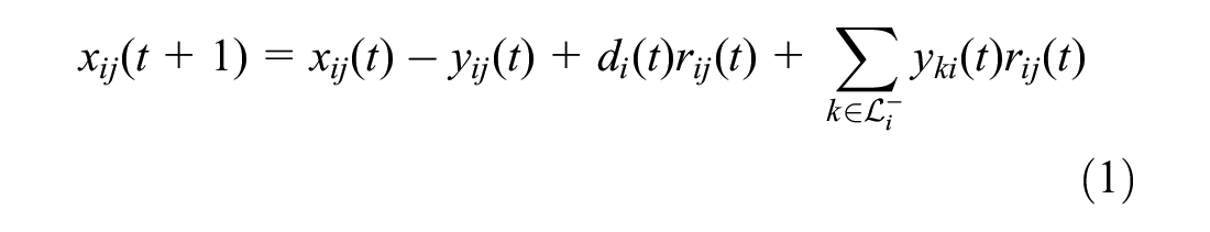
In Equation 1,

Equation 2 means that the number of vehicles leaving the intersection can be at most the number of vehicles waiting at that intersection. However, if the capacity of the intersection
Max-Pressure Controllers
In this section four max-pressure controllers are defined mathematically, and the basics of their functions are explained. These different controllers are defined by their weight function, which will later be used to assign green time to turning movements.
The link queue and movement queue controllers were chosen for study because they have each been proven to be throughput maximizing ( 1 , 4 ). However, it is still important to study the behavior of these controllers in large-scale networks to see if other properties such as travel time and number of waiting vehicles are equivalent.
The density queue max-pressure controller was also chosen for study because of its unique properties which help to prevent congestion from propagating backward through the network ( 6 ). Though maximum throughput has not been proven for this controller, it has been shown in simulation to perform well in comparison with other max-pressure controllers.
Link Queue Max-Pressure Controller
The link queue max-pressure controller was developed by Wongpiromsarn et al. (
4
). In the link queue max-pressure controller, the weight (or pressure) of each phase is calculated by the difference between the queue length at the link entering the intersection and the queue length at a downstream link. Equation 4 defines this relationship for any movement between links


Density Queue Max-Pressure Controller
For the density queue controller, we need to define a new weight equation. This equation looks very similar to Equation 4 but replaces the queue length with a more complicated value of pressure

The pressure depends on the jam-density of the link (
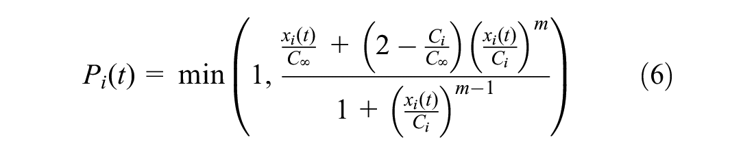
Figure 1 shows the shape of the pressure function. A queue of vehicles on a shorter link will have a higher pressure than the same number of vehicles on a longer link. In addition, when each of the links is filled with vehicles, the pressure will always be 1 regardless of the length of that link. Beyond that, Gregoire et al. ( 6 ) constructed this function to be near linear when there are only a few vehicles on each link to preserve the “fairness” of the policy, but to increase more rapidly as the link gets filled since each additional vehicle poses an increasing problem.
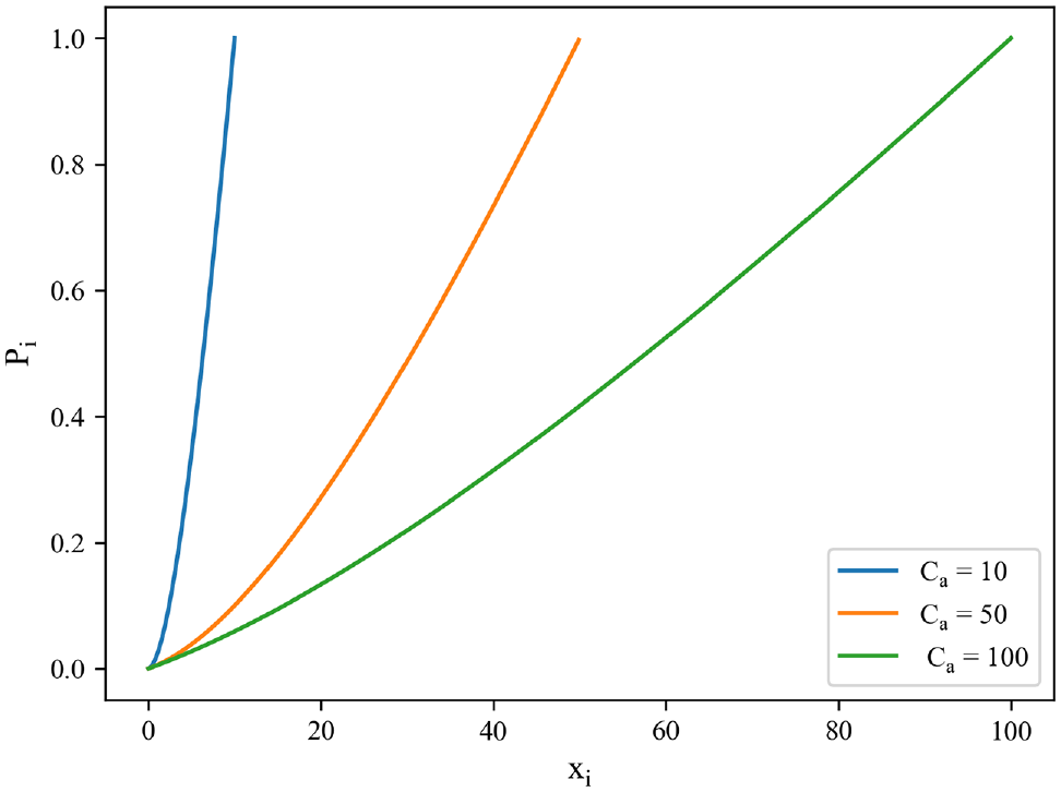
Graph of the pressure at an intersection caused by a queue for cases when the link has sufficient length to contain 10, 50, and 100 vehicles.
Movement Queue Max-Pressure Controller
The movement queue max-pressure controller incorporates the turning ratios (


This equation provides additional information since it differentiates between vehicles making different downstream movements. Generally, incorporating vehicles further downstream can help the controller maximize throughput by sending vehicles down links which are less congested. Adding the turning ratios can help keep narrow down how the congestion will form downstream so it can be prevented upstream. The turning ratios were determined by finding the user equilibrium for trips in the network and using these ratios as an estimate of the actual ratios.
Assigning Green Time
Once all the weight functions are defined, they need to be converted from turning movements into phases. Each phase provides green time to one or more turning movements and each turning movement can be activated by multiple phases. Each phase is assigned a weight based on the weights of all the turning movements that make up that phase.

In Equation 9, we find the weight of phase

Equation 9 will be used by all controllers to convert the weight of each turning movement to the weight of a phase. Finally, there are three methods of signal timing utilizing those weights, the non-cyclic, cyclic, and semi-cyclic controllers.
Non-Cyclic Max-Pressure Controllers
In the non-cyclic version of max-pressure control, the weight functions are used to assign green time to the available green phases. The controller activates phase

In other words, at every time step, the phase with maximum weight will be set as the green phase. If the chosen phase is the same as the previous phase the yellow and all-red intervals can be skipped. Otherwise, the signal activates the yellow and all-red phases before activating the new phase. Only after that new phase is complete will the weights be recalculated for the next time step. This sets a default minimum green time of one timestep (generally 15 s), but sets no maximum green time.
Since this is the non-cyclic version this same computation is made at every time step and the phase of maximum weight is chosen independently. This means that the same phase can be activated for longer or more often if a phase is busy, and less busy phases can be ignored entirely. On the other hand, this can cause longer waits at low pressure phases and it can cause the controller to cycle back and forth rapidly if queues are of similar lengths on different phases. Unfortunately, this can lead to additional loss time on the yellow and red intervals.
Another drawback of the non-cyclic controller is that it can sometimes create gridlock, even at relatively low demand ( 22 ). This can be caused when there are nearby links with very different lengths. The short links can get filled with vehicles and cause queue spill-back, and still never receive a green light because of their low jam-density. This problem is addressed with the cyclic controller which will eventually give green time to all links and break up the gridlock.
Cyclic Max-Pressure Controllers
The cyclic max-pressure controller is defined by the same weight equation as the non-cyclic version. Then, the phases are activated in order. However, in this case one more step must be taken to determine the activation length of each phase (called a split in conventional control). A logit model is used to determine the length of the phase using the weight.

This model can be run for each phase and will set a proportional green time. The term
Unlike the non-cyclic version, this controller will activate every phase in every cycle. This behavior is also distinct from cyclic actuated controllers which are allowed to skip phases. Activating all phases will ensure that shorter queues also get some green time, but if there are no vehicles or very short queues it could waste green time on empty links. In addition, if the total green time is too short, the queues may not be cleared at some links, and time can be lost from additional yellow and red phases as the signal cycles too quickly.
Semi-Cyclic Max-Pressure Controller
As the cyclic and non-cyclic versions of the controllers were discussed, some benefits and drawbacks were noted. To solve some of these concerns, a novel semi-cyclic controller is introduced. The semi-cyclic controller is designed to work like the non-cyclic controller much of the time. However, we add an additional step to the process to make sure that each phase will eventually be actuated.
For each intersection, we calculate a maximum number of steps before each phase must be activated,

Once the maximum number of time steps between phase activations is determined, phase

If there exists a phase
Microsimulation in SUMO
Several of these controllers have been proven to maximize throughput, but others have not. In addition, all the controllers need to be investigated beyond throughput to see if travel time or number of waiting vehicles are affected by the chosen controller. To investigate these impacts the microsimulation software Simulation of Urban Mobility (SUMO) was chosen.
Many previous studies have used only a few intersections, or an artificial network to study max-pressure controllers. However, a larger and realistically structured network has better potential to encounter problems that may come up in real traffic scenarios. For that reason the downtown Austin network (shown in Figure 2) was chosen for simulation. This network is composed of 1186 links, 506 total intersections, and 167 signalized intersections. In addition, to replicate the network as closely as possible, only the existing phases of the signals are used. Though there could be some combination of phases that works better with max-pressure controllers, this is outside the scope of this study and our controllers can only modify the green time of the existing phases. Finally, the demand used in the analysis is 40%, 60%, and 80% of a 48,180 vph (vehicles per hour) demand, corresponding to 19,272, 28,908, and 38,544 vph. This demand is based on the real Austin demand of 62,836 vehicle trips over the 2 h morning peak period. This traffic is scaled up and down to show how the controllers perform differently, but the origin–destination proportions are left the same. The University of Texas at Austin Network Modeling Center provided the demand data calibrated to match observed counts in 2011, as well as data used to create the network, determine existing phase configurations, and program the signal timings.
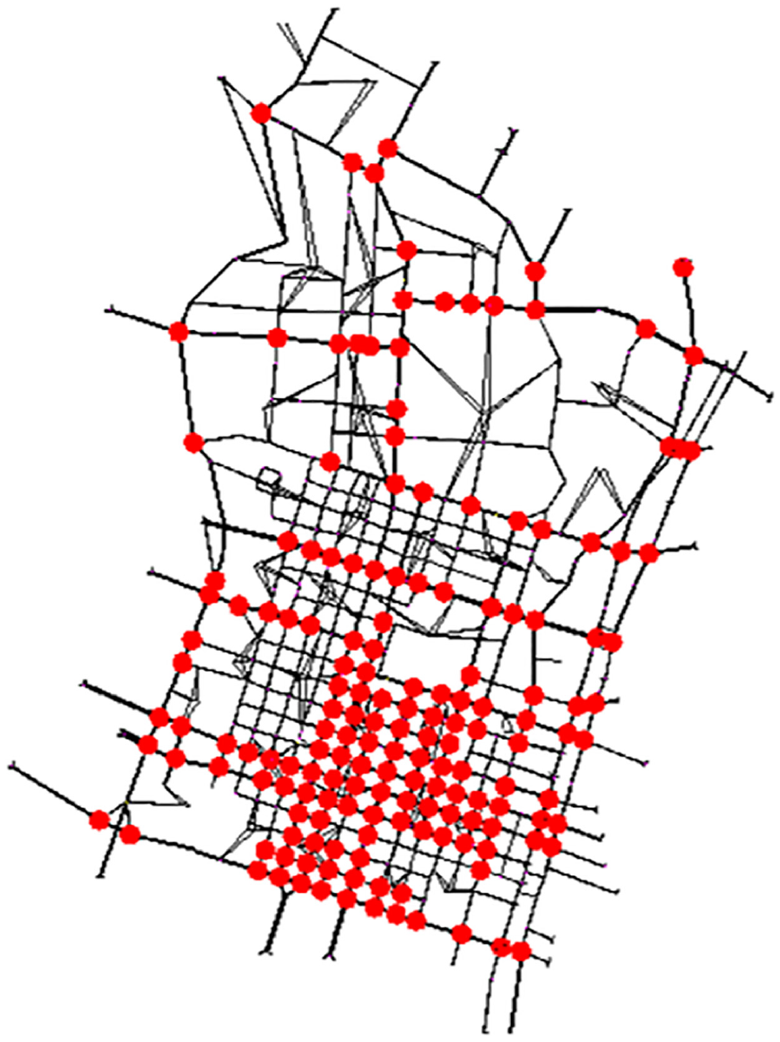
Downtown Austin network shown in SUMO.
The use of a realistic network causes some additional problems for max-pressure controllers. In particular, lanes which have queues using multiple movements such as a shared left and through lane make turning movements indistinguishable. For that reason, in this study aggregate turning movements are used when necessary. In these cases, the queue lengths
Another concern is conflicting movements such as a phase where through movements are protected and left turners are permitted. This is common in real traffic scenarios but may be a challenge for max-pressure controllers. Since it may take much longer for left turners to find an acceptable gap it can take much longer to clear queues of left turners. These problems can be exacerbated by shared through–left lanes even when the proportion of turning vehicles is small. In this study, the saturation flow rate takes into account whether movements are permitted or protected.
One feature of max-pressure control worth noting is that multiple phases can activate the same movements. For example, consider a structure with a left-turn lane and two through lanes in one direction. If there is a phase where left turns are permitted and through traffic is protected the traffic in all lanes will be used in the weight function. However, for a protected left-turn phase with no through traffic, the through traffic will not be included in the weight. Generally, this will cause the weight of the protected left-turning phase to be very low compared with the phase allowing through and permitted left-turning movements. This will cause the controller to choose the through and permitted left-turn phase over the protected left, which can cause a buildup of left turners.
The SUMO software allows all the network and phase information to be imported along with a preset list of vehicles and routes. These are loaded into the network throughout the simulation in preset proportions. The activation of the phases can be controlled using the Traci interface in Python. This interface allows the phases to be altered in real time throughout the simulation based on the queue lengths and delay information. Though the simulation is run for 3 h, numerical data are taken starting 15 min into the simulation and ending after 90 min. This gives the network time to populate with vehicles before the averages are taken and it stops just as vehicles stop entering the network at 90 min in. Some graphs also show the entire simulation so the warm-up and cool-down periods can be observed.
Results
The results of this study are broken up into two parts. First, simulations using each type of controller are shown for a single intersection. This allows for a more careful analysis of their behavior. Next, the non-cyclic, cyclic, and semi-cyclic controllers are tested with variation to some of the parameters, including the computation frequency, total green time, and semi-cyclic multiplier
In all plots of travel time, we plot the mean travel times of vehicles that arrived in a 1 min period for each minute in the simulation. Similarly, the plotted number of waiting vehicles is the mean of the number of waiting vehicles at each timestep for 1 min. These measures are effective in demonstrating the progression of congestion over time as the simulation runs. The average number of waiting vehicles at each timestep also shows whether more vehicles are entering or leaving the network over time, which demonstrates the stability of the controller. To get average travel time for the entire simulation, the mean travel time is found for all vehicles arriving between 15 and 90 min when the demand is constant and the network is populated. Similarly, to find the average number of waiting vehicles, the mean number of waiting vehicles at each timestep is found for all timesteps between 15 and 90 min.
Observations at a Single Intersection
Using network wide averages, it is difficult to see why different max-pressure controllers behave the way that they do. For that reason, the new semi-cyclic controller is examined at a basic three-legged intersection (shown in Figure 3). There are several intersections with similar geometry in the larger network, and lessons learned from this intersection can be applied to more complicated geometries. To simplify the analysis, only the link queue max-pressure controller is used, and only the trends in travel times are observed.
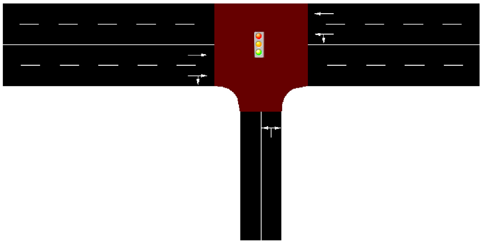
Basic three-legged intersection generated in SUMO.
To see how the semi-cyclic controller behaves at different levels of demand, we can set the demand for each movement through the intersection and observe how the cyclic, non-cyclic, and semi-cyclic controllers respond. The first scenario will keep the traffic turning onto and off the side street low. First, we set this value to 36 vph for all four turning movements (right and left turns onto and off the side street). On the through street, we can set the demand to 360 vph in each direction.
In Figure 4, we see evidence of the very low demand of the turning traffic. We see a few peaks in the travel time plot of the non-cyclic controller indicating the few places where turning traffic has sufficient weight to get a green light. We also see the much more periodic peaks of the cyclic controller where it has stopped the through traffic to let turning vehicles go. In this case the semi-cyclic controller finds a balance between the two, giving green time to turning vehicles more often than the non-cyclic controller but not holding up through traffic as much as the cyclic controller. However, overall, these graphs are chaotic and do not show any clear superiority for any type of controller.
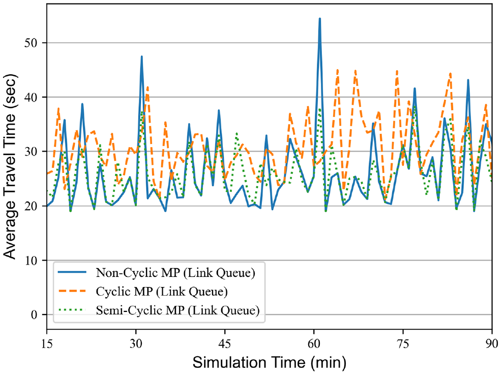
Three-legged intersection travel time with 360 vph through traffic and 36 vph side street traffic.
Figure 5 has the same demand on the side street but doubles the demand of the through traffic. With more through traffic, there is not enough demand on the side street to trigger the non-cyclic controller and we see very long wait times for the side street traffic. These long waits are shown by the peaks in the non-cyclic controller waiting vehicle plot. On the other hand, the cyclic controller gives some green time to these vehicles, slowing down the through traffic slightly but leaving the waiting times on the side street much shorter. The semi-cyclic controller follows this pattern since it has a set maximum waiting time for head-of-line vehicles on the side street (in this case six time steps or 90 s). This maximum waiting time keeps the minute average travel times much lower than the non-cyclic controller is able to achieve.
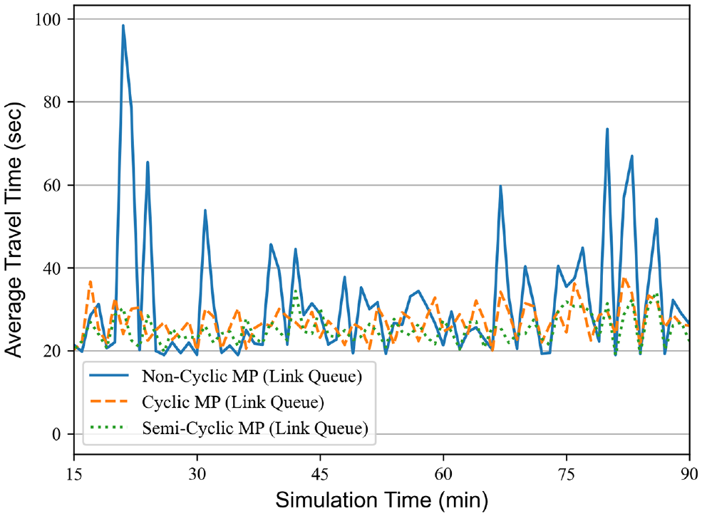
Three-legged intersection travel time with 720 vph through traffic and 36 vph side street traffic.
Figure 6 shows what happens with very high through traffic and high traffic turning off the side street (720 vph). Turning traffic onto the side street remains at 36 vph. In this case, the semi-cyclic and non-cyclic controllers behave exactly the same. This is because the non-cyclic controller is calling each phase often enough that the waiting time for the head-of-line vehicle is never larger than 90 s. In addition, we can see that the cyclic controller performs slightly worse than either of these.
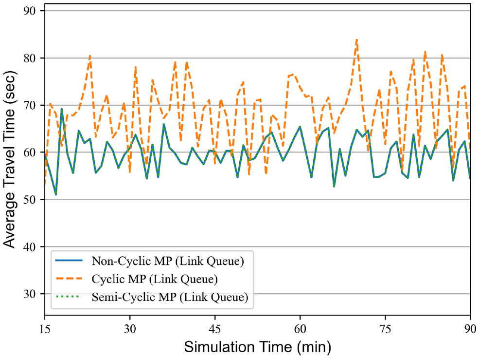
Three-legged intersection travel time with 720 vph through traffic and turning movements out of the side street, and 36 vph onto the side street.
We can also see one of the biggest problems with the cyclic controller. There are periods of very low travel times and periods of very high travel times and the distance between each of the peaks is 3 min. However, the cycle length is 90 s. What this shows is that the second phase gets less green time than it should since that queue has had green time more recently. This does not allow all the vehicles to be released (increasing the waiting times of those held back) and it then must allot more green time to that phase the next cycle. For that reason, we can see that every other cycle there is a jump in the average travel times because of vehicles turning off the side street that were required to wait two cycles.
Though there are many other traffic patterns and intersection geometries that can be tested, these simple cases show some very important properties of the semi-cyclic controller. When the demand is coming into the intersection in sufficient proportions for the non-cyclic controller to serve all approaches well, the semi-cyclic controller will mirror its behavior. However, when the cyclic controller outperforms the non-cyclic controller (generally because of approaches with very low demand), the semi-cyclic controller can act similarly to the cyclic controller and give some green time to all movements.
This simulation was run many times with variations on the demand patterns above. No situation was found where the semi-cyclic controller was outperformed by both the cyclic and the non-cyclic controller. Often, all three performed comparably, and when one performed better the semi-cyclic controller mirrored that behavior. These patterns explain why the semi-cyclic controller performs comparably and sometimes slightly better than the non-cyclic controller in a large network. Based on the results on the network below, we can see that the cyclic controller performs worse than the other two variations. This suggests that cases with relatively symmetric and high demand like Figure 6 shows might be common. However, the non-cyclic and semi-cyclic controllers are not behaving exactly the same over the whole network which proves that there are times when the non-cyclic controller has unacceptably long waiting times.
Large-Scale Simulation
To look more deeply at each of the controllers, it is important to compare the effects of changing the weight function of each max-pressure controller with the way in which green time is assigned. The easiest way to observe this difference is to look at a plot of the average number of waiting vehicles and travel times at a medium demand of 28,908 vph.
Figures 7 and 8 clearly show the vast gap in performance between the cyclic and non-cyclic controllers. While there is some difference between the max-pressure weight functions, the differences between the way green time is assigned tend to have more importance. That said, there are some features of the cyclic controller such as constraints on head-of-line waiting time for vehicles that are replicated in the semi-cyclic controller. These plots show that even with these features, the semi-cyclic controller performs very comparably to the non-cyclic controller in a network wide scenario.
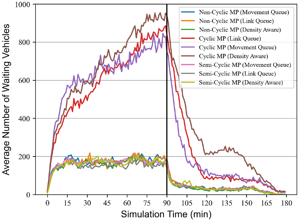
Comparison of number of waiting vehicles for 28,908 vph demand.
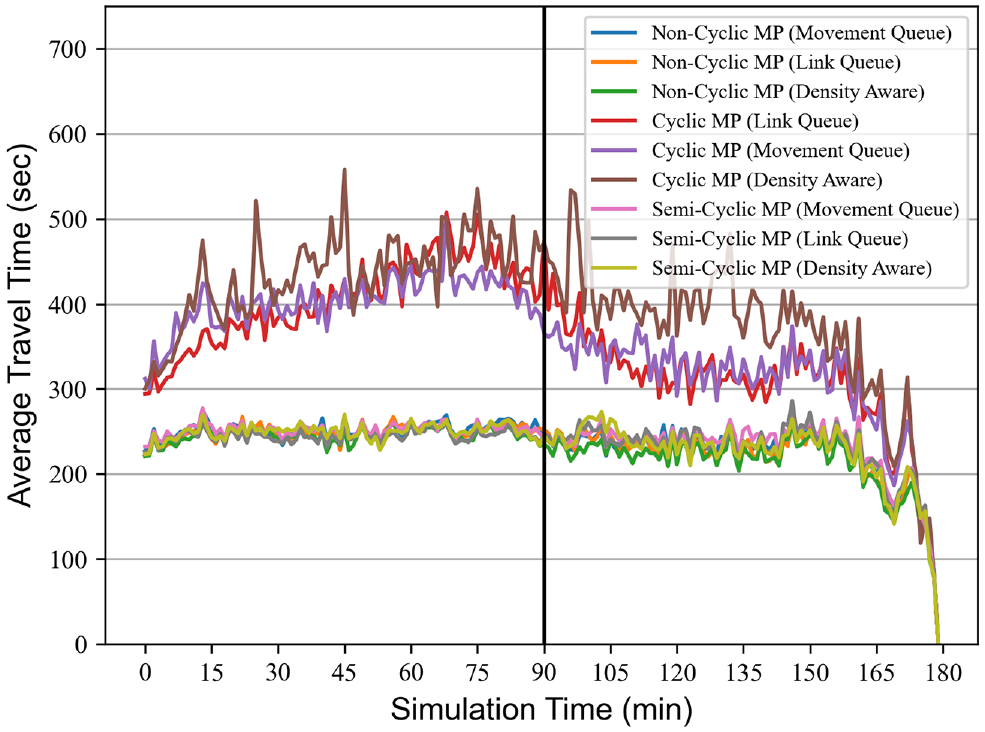
Comparison of travel times for 28,908 vph demand.
To look more closely at some additional scenarios, Tables 1, 2, and 3 show the average travel time and average number of waiting vehicles in simulations with low, medium, and high levels of demand. Each table shows a range of computation frequencies for the non-cyclic controller and a range of green time multipliers for the cyclic controller (a green time multiplier of 0.5 means the cycle length is half that of the fixed-time controller). In addition, the computation frequency and the semi-cyclic multiplier
Average Travel Times (in Seconds) and Number of Waiting Vehicles for All Max-Pressure Controllers under Demand of 19,272 vph
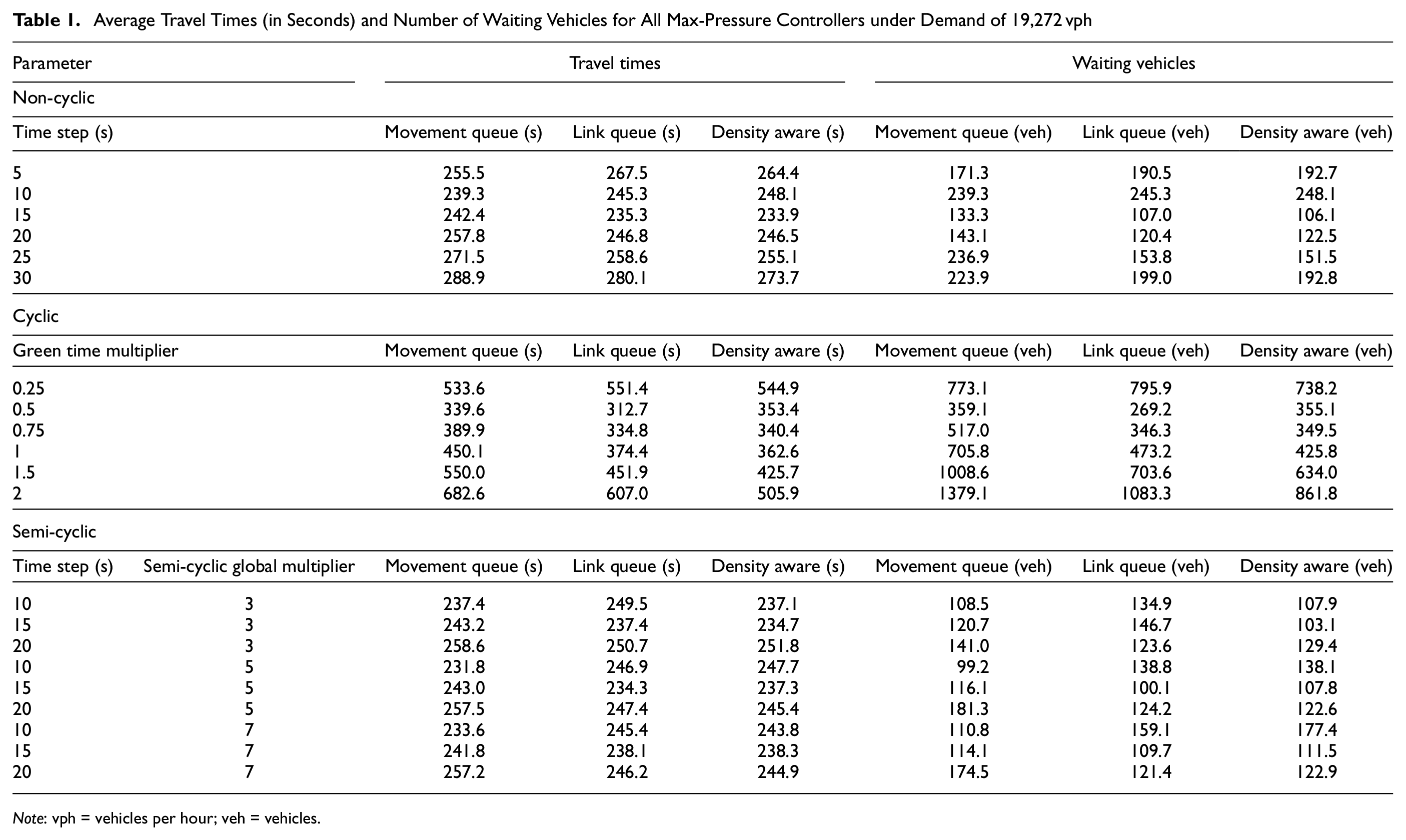
Note: vph = vehicles per hour; veh = vehicles.
Average Travel Times (in Seconds) and Number of Waiting Vehicles for All Max-Pressure Controllers under Demand of 28,908 vph
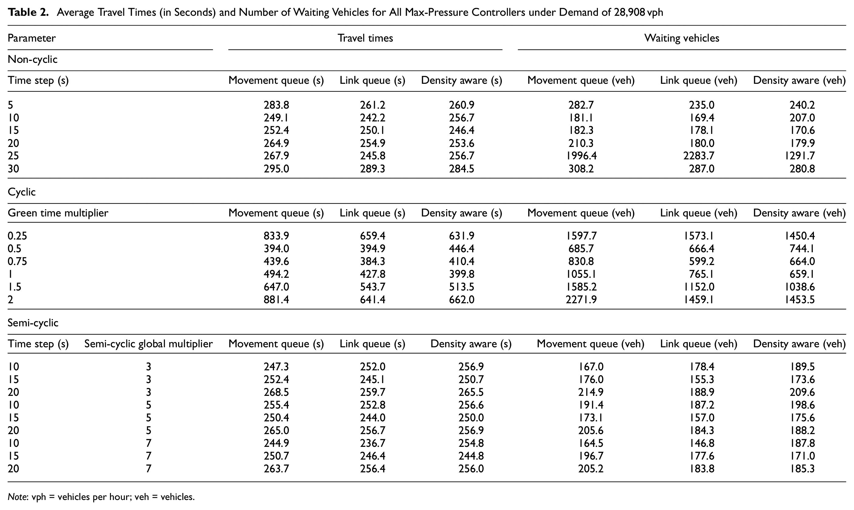
Note: vph = vehicles per hour; veh = vehicles.
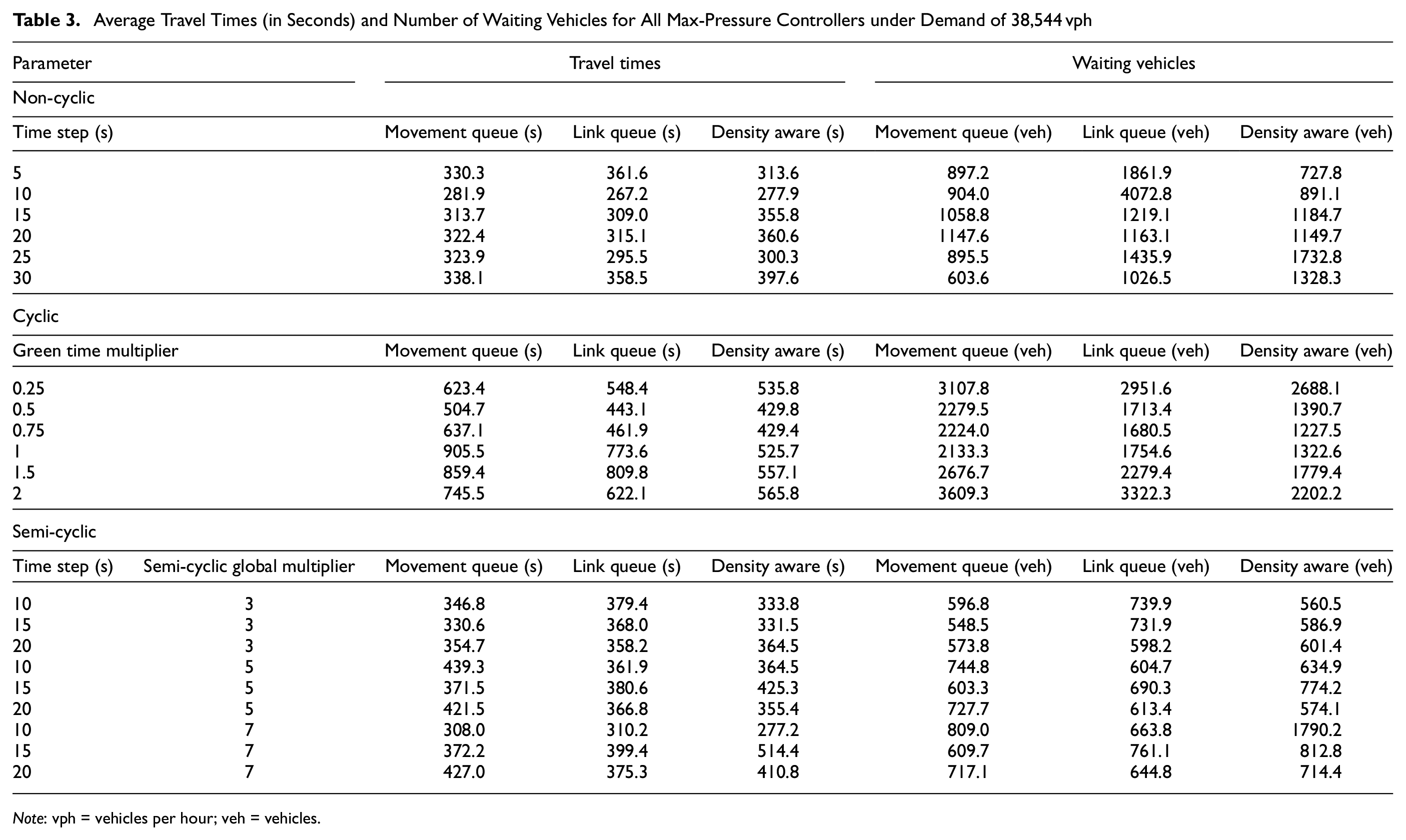
Average Travel Times (in Seconds) and Number of Waiting Vehicles for All Max-Pressure Controllers under Demand of 38,544 vph
Note: vph = vehicles per hour; veh = vehicles.
At low demand, we can see stark differences between the cyclic controller and the non-cyclic and semi-cyclic controllers. The cyclic controller has much higher travel times and number of waiting vehicles. For the non-cyclic controller, we see the best range of time steps in the range of 10 to 15 s. The increase in travel times as the time step increases suggests that each phase is being given more time than is necessary to release the queue, so time is being wasted. On the other hand, time steps at only 5 s are causing delays because the ratio of yellow and red time to green time is increasing. Similar patterns can be noted for the cyclic controller. A very short cycle time causes delays and high numbers of waiting vehicles, as do very long cycle lengths.
The semi-cyclic controller shows very consistent results with different values of the multiplier
When the demand is increased to 28,908 vph in Table 2, the clearest effect is that some of the values of waiting vehicles have jumped much higher for both the cyclic and non-cyclic controller. This suggests that there is either gridlock or queue spill-back somewhere in the network. By comparison, the semi-cyclic controller never reaches gridlock and the number of waiting vehicles is consistently lower. Travel times for the semi-cyclic controller are again very similar to the non-cyclic controller. However, since there are higher numbers of waiting vehicles, arrival times for the non-cyclic and cyclic controllers will tend to increase with simulation duration. Likely, gridlock formed toward the end, so did not have time to affect average travel times significantly since times are only counted when vehicles arrive at their destination. Increasing the demand in Table 3 will exacerbate this trend further.
A demand of 28,908 vph is significant, but ideally, the controllers should be able to stabilize this demand since it is still less than the downtown Austin peak hourly traffic. By ruling out values of parameters that are clearly unstable, we can see some obvious trends. The time step for the non-cyclic and semi-cyclic controller should be kept between 10 and 20 s. The cyclic green time multiplier should be kept between 0.5 and 1. Ideally, each of these parameters could be optimized at each intersection individually.
Under a demand of 38,544 vph, there is an interesting comparison to be made between the non-cyclic and semi-cyclic controllers. The non-cyclic controllers tend to have slightly shorter travel times, but larger numbers of waiting vehicles. It is likely that this trend would cause the non-cyclic controllers to do worse over time since there are likely still many vehicles in the simulation by the end of 90 min with very long waiting times. By contrast, any remaining vehicles in the semi-cyclic simulation would have had very little waiting time.
Figures 9 and 10 show the progress of the simulation. These figures show that the travel times of vehicles that arrive in the first 90 min are low for the non-cyclic controller, but there is gridlock forming in the network even in the first 90 min as indicated by the higher number of waiting vehicles in Figure 10. Some vehicles never arrive at their destination after 3 h. Travel times are lower because we can only determine the travel time for vehicles that have exited. Though the semi-cyclic controller has slightly longer travel times throughout most of the simulation, both the movement queue and link queue controllers drop to zero waiting vehicles by the end of the simulation.
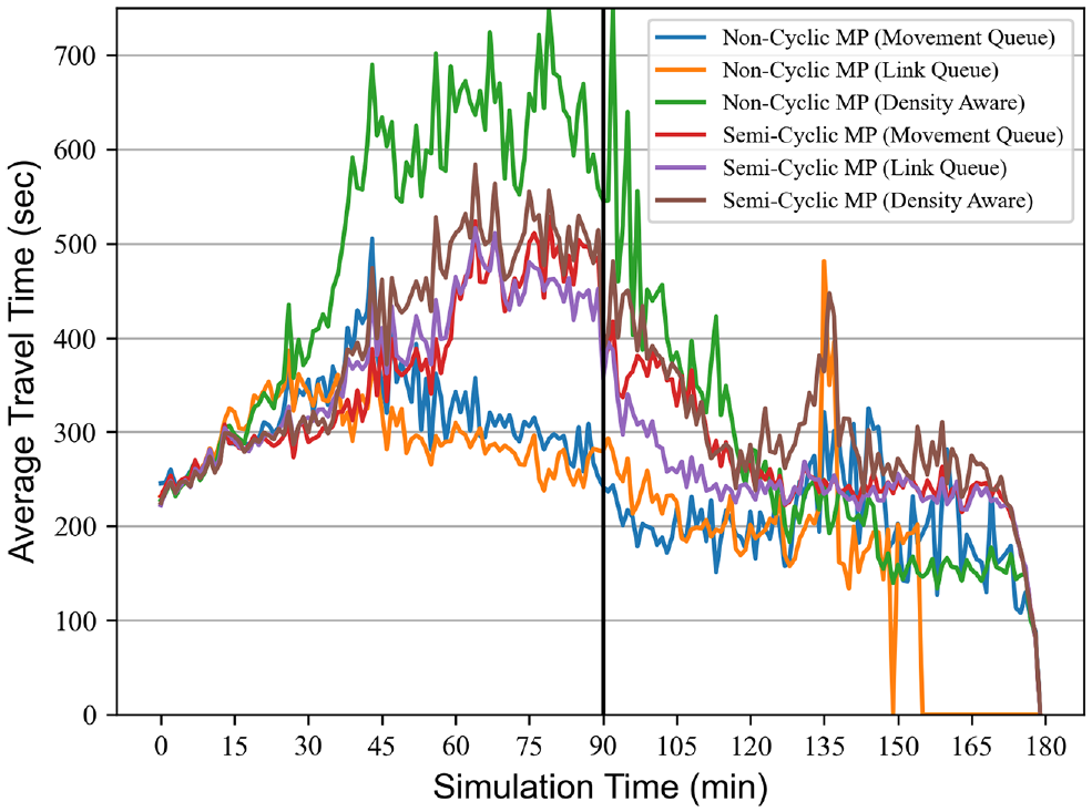
Comparison of travel times for 38,544 vph demand. Based on a time step of 15 s and semi-cyclic global multiplier of 5.
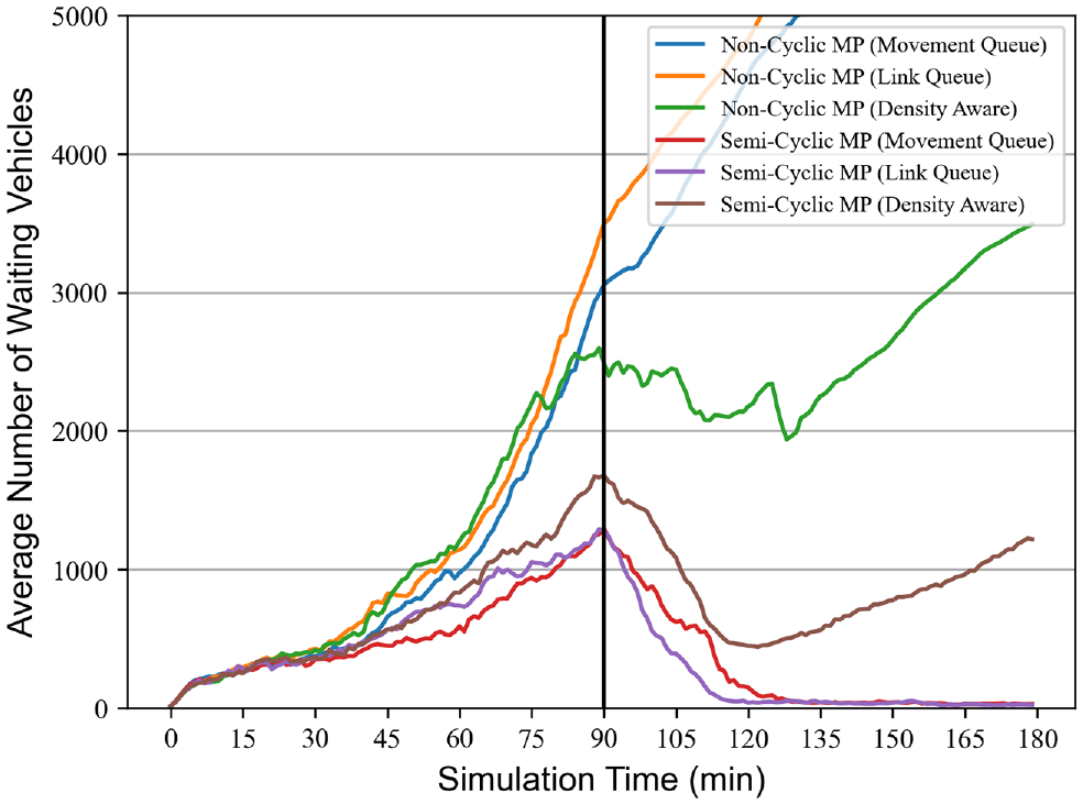
Comparison of number of waiting vehicles for 38,544 vph demand. Based on a time step of 15 s and semi-cyclic global multiplier of 5.
Based on all these different demands, it seems that a green time multiplier which is less than 1 is best. Generally, all controllers do better in a range of 0.5 to 1. These results are surprising. Since the fixed-time controllers are optimized, a multiplier of 1 was expected to be best so that the cyclic controller operated with only small changes to the behavior of the fixed-time controller. Instead, the cyclic max-pressure controllers behave slightly better at lower cycle lengths.
The behavior of the cyclic controller can in part be explained by when the timing is calculated. Since the pressures are always calculated at the end of the cycle, whichever phase is last will generally have a much smaller queue. This will result in a small fraction of the green time. However, by the time that phase occurs next a much larger queue will have accumulated that cannot be relieved by such a short green time. Finally, on the next cycle that phase will be given a larger amount of green time which will allow the queue to exit but leave only a very small queue which will not receive enough green time for the next cycle.
Conclusion
This paper tested nine different combinations of max-pressure weight functions and methods of assigning green time. The numerical results show that there is a much larger difference in performance between the cyclic and non-cyclic max-pressure controllers than between any of the studied weight functions. For that reason, more research needs to be done on methods of assigning green time. This study developed a new class of controller, the semi-cyclic controller, which attempted to mitigate some of the challenges with the non-cyclic and cyclic controllers.
A look at a single intersection shows that as demand changes at a single intersection, the semi-cyclic controller is able to adapt. It successfully follows the travel time and waiting vehicle patterns of whichever controller does better. Over many intersections, the simulations show that the semi-cyclic controller performs much better than the cyclic controller and sometimes slightly better than the non-cyclic controller.
Finally, some concerns with the non-cyclic controller are that it has the possibility to create gridlock (even at low demand) and that it can create very long waiting times for low demand links. However, the semi-cyclic controller addresses those problems. Gridlock is less likely to occur since, as with the cyclic controller, all phases will eventually be cycled through. In addition, the semi-cyclic controller sets a maximum waiting time for head-of-line vehicles. Thus, the controller presents a more equitable distribution of waiting times at intersections while retaining a performance closer to that of the non-cyclic than the cyclic controllers. Future work should analytically compare the congestion properties of these three controllers to explore general gridlock occurrence, but that is outside the scope of this simulation study.
In addition to performing worse than the non-cyclic controller, the cyclic controller has some problems with when the green time is calculated. Generally, the last phase gets less green time than it should since that queue has had green time more recently. Over time this causes the controller to perform worse. The semi-cyclic controller solves that problem. The computation is performed every 15 s and the queue with highest weight is chosen instead of calculating the weights all at once at the end of a cycle. However, it is able to retain some of the properties of the cyclic controller since it is eventually forced to cycle through all phases.
Previous literature has focused on the weight function as a way to optimize max-pressure signal control. This research suggests that more focus should be given to how green time is assigned based on the weight functions. We suggest that future research should examine additional cyclic structures that perform better than the logit model. In addition, structures like the semi-cyclic controller could benefit from more careful distinction between turning movements and phases. A controller that required turning movements to be activated each cycle or after a maximum number of phases (as with the semi-cyclic controller) but did not require that each phase be activated could see additional improvements, as could a formulation of the cyclic controller that set a minimum green time or that was allowed to skip phases. However, the stability of these different controllers would have to be separately proven. We hope that research in this direction will help to find and alleviate additional concerns with max-pressure controllers so they can begin to be confidently implemented by traffic engineers.
Footnotes
Author Contributions
The authors confirm contribution to the paper as follows: study conception and design: Chen, Robbennolt, and Levin; data collection: Chen and Robbennolt; analysis and interpretation of results: Chen, Robbennolt, and Levin; draft manuscript preparation: Robbennolt and Levin. All authors reviewed the results and approved the final version of the manuscript.
Declaration of Conflicting Interests
The author(s) declared no potential conflicts of interest with respect to the research, authorship, and/or publication of this article.
Funding
The author(s) disclosed receipt of the following financial support for the research, authorship, and/or publication of this article: We gratefully acknowledge the support of the National Science Foundation, Award No. 1935514.