
Abstract
Different individuals may move to different regions over time, but every individual has several fixed travel positions or unique travel patterns. Predicting destinations of each individual facilitates traffic demand management, which has great research value. Based on the data of multi-day GPS and passengers’ travel survey, a hidden Markov model (HMM) is employed in this paper to predict trip destination for weekdays and weekends. Firstly, the habit of destination choice among consecutive days and weeks can be discovered by identifying frequently visited destinations. Then, on the basis of Viterbi algorithm, this paper takes frequently visited destinations as one of the factors of the predicting process and constructs a travel destination prediction model based on HMM. Then, the HMM is calibrated with Baum-Welch algorithm and passengers’ travel destination characteristics are effectively analyzed. Finally, the HMM was compared with several classical algorithms. The results show that the place of residence and work are the most probable activities to occur and workplace dominates the activities when duration is longer than 8 h. Moreover, the results of frequently visited destinations identification indicate that the patterns of destination choice on weekdays and weekends are different from each other. In addition, the results show that the prediction accuracy on weekdays is higher than that on weekends and HMM outperforms other prevailing algorithms. The method proposed in this paper can be applied to real-time travel navigation applications, as well as supporting health and safety fields, such as epidemic prevention and control.
Keywords
Based on the global positioning system (GPS) data of individuals in social network applications, the main factors affecting individual travel decisions can be studied, and the transfer rule of individual travel and the modeling mechanism of travel behavior can be mined, so as to achieve the goal of predicting individual travel location at the next moment. At different time points, different traveling individuals may move to different regions. Each traveling individual has several fixed resident positions or unique travel patterns. Generally, individuals will preferentially move near their resident areas, but there is a certain probability that they will move to other locations ( 1 ). It is of great research value to analyze and predict individual behavior by counting the location of each individual at different time points. In general, the real location of most individuals will have its own unique category label, which directly reflects the natural attributes and commercial activities of this location. In real life, people tend to have different preferences for travel locations. For example, people who love food often visit different dining locations. Tourist attractions are often the first choice during holidays. Therefore, the personalized preferences of moving objects to travel destinations can be modeled based on the historical locations visited by individuals.
Travel destination prediction is the focus of research in the field of individual behavior analysis and has profound significance for traffic flow prediction. Modeling and analysis of individual behaviors at the micro level is helpful to accurately understand the generation mechanism and evolution process of urban traffic phenomena from the macro level, which can better lay a good foundation for real-time prediction of crowd flow in urban traffic ( 2 ). At the same time, travel destination prediction can generate great economic value in the application of location recommendation. Based on the historical location records on social networks and the ratings on social applications, users can be recommended the places they are most interested in. For example, restaurants and shopping centers that meet users’ needs can be recommended to users effectively and reasonably. At the same time, enterprises can deliver personalized commercial advertisements to users to improve the popularity of products. In addition, the prediction of travel destinations is of great practical value in health and security fields such as epidemic prevention and control. Traditional epidemic monitoring methods are lagging behind to some extent. In recent years, social networks have provided a new monitoring method for epidemic prevention and control. Significantly reducing people’s willingness to travel and reducing the proportion of people in the same area in contact with each other can greatly slow down the spread of an epidemic, which has profound practical value in the epidemic prevention and control research. In addition, individual mobility is also key to epidemic prevention and control. Novel Coronavirus was discovered in 2019 as a result of a case of viral pneumonia in Wuhan, China, and was named by the World Health Organization on January 12, 2020. During China's Spring Festival travel rush in 2020, large-scale population movements accelerated the spread of the epidemic in time and space. However, the population return across the country after the Spring Festival still poses a huge challenge to the prevention and control of the epidemic in China. Therefore, a comprehensive understanding of the flow characteristics of individual travel and an accurate prediction of the travel location can play a positive role in the prevention and control of the epidemic.
The remainder of this paper is structured as follows. The next section introduces the literature review. In the section after that, the methodology is presented. The penultimate section analyzes a case study, including data description, data analysis, model calibration, and results. Finally, the conclusions and discussions are given.
Literature Review
Trip destination can be separated into different categories. The categorization: “home,”“work/school,” and “other” is the simplest and most common classification strategy. Alexander et al. divided trip destination into home, work, and other ( 3 ). Home was the category with the greatest number of visits from 7 p.m. to 8 a.m. Work was the greatest distance from home and other was otherwise. Increasing the number of categories provides more specific trip destinations. However, this also increases difficulties of inference and prediction. Iqbal and Pao achieved 88.7% accuracy when differentiating between seven trip destinations ( 4 ). With more types of travel destination, the accuracy of model prediction has become an important index to detect the suitability of the model. For 12 distinct trip destinations, the overall accuracy that Oliveira et al. reached was only 65% ( 5 ). Nevertheless, these accuracies were dominated by home or work trips, which accounted for approximately one-third of total trips. With the help of the Google Places API, which is a type of online and real-time location-based query service, Ermagun et al. achieved 67.14% overall prediction accuracy by using the random forest (RF) algorithm when differentiating between five trip destinations other than home and work ( 6 ).
Recent researches have advanced the field through more advanced algorithms via map-matching, sub trajectory synthesis, and other data mining approaches. These methods greatly increase predictive accuracy, but they require en route information and do not report higher predictive accuracy at the beginning of the trip. To increase the baseline accuracy, new methods and data elements are needed. Yao et al. extracted the time, location, text, and other features of individual trips, and modeled the index of real geographic locations in the grid through a cyclic neural network to model the movement rules of individual trips ( 7 ). In addition, Bingbing et al. proposed figure convolution neural network prediction in individual travel destination and has made significant achievements, using graph data structure to store the social network—each node stores the individual characteristics of spatial-temporal travel information, through to the node end-to-end nonlinear characteristic information and structural information to automatic learning—enhancing the ability to model individual behavior ( 8 ).
In addition to the above research methods, there is a new machine learning method for travel destination prediction. The hidden Markov model (HMM) is a type of machine learning techniques that has accomplished great achievement in the fields of computer vision. Krause and Zhang developed a Markov model to predict destination with the data of GPS and land use ( 9 ). A baseline tiered time origin model was developed using the Markov chain approach and then a machine learning technique derived the trip destination. Zong et al. offered HMM to estimate number of trips ( 10 ). By introducing support points, the trip model is developed with HMM. Han and Sohn imputed trip traces from travel smart-card data ( 11 ).
The HMM approach proposed for this research has been previously applied in other domains of transportation research, but it is still worth exploring in the application of travel prediction. This paper uses the time threshold of 4 min to identify midway stops, and the ending point of every trip is recorded as its trip destination. Then, the frequent travel destination is counted—if the visit frequency of a trip destination is not less than 0.13 times and 0.28 times per day for weekdays and weekends, it can be taken as a frequently visited destination. Then, Markov model parameters (initial probability, transition probability) are calculated. Finally, Viterbi algorithm in dynamic programing (DP) is used to calculate the probability of individual check-in at different locations.
Methodology
A Markov chain and a Gaussian mixture are mixed together to form an HMM ( 12 ). A Markov chain describes the state of transition between two consecutive activities of a traveler. The present study adopts to the basic assumptions of HMM, which are the homogeneous Markov hypothesis and the observation independence hypothesis.
The procedure of imputing the activity sequence of trip chains based on an HMM is summarized. Firstly, the sample trip chains are extracted from multi-day GPS data and the number of potential activities is determined. Secondly, the possible number of clusters is determined, and feature data are collected for every hidden activity within the sequence of activities for trip chains (Figure 1). The next step is to implement a solution algorithm for estimating the parameters of an HMM and to map each state with them by investigating the estimated parameters. Finally, using the parameters, the most probable sequence of activities is imputed for trip chains.
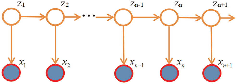
The mechanics of determining states and observations behind a hidden Markov model (HMM).
Travel Destination Prediction Model
Destination prediction is advancing quickly because of the availability of accurate moving point data via multi-day GPS loggers, transmitting GPS systems, and smart phone applications. Modeling has become increasingly accurate for the correct estimation of a trip from its origin to its end. By applying trip destination estimation before destination is predicted, a more accurate destination can be made by giving a set of possible locations that would achieve the same trip destination.
Before the trip destination prediction based on HMM, firstly, it is necessary to identify the frequently visited destinations of the actual travel activities, then take frequently visited destinations as one of the predictor variables of the HMM to predict trip destination. Wang proposed the time threshold of 4 min to identify midway stops ( 13 ). That is, the trip dividing condition is leg time no less than 4 min. For example, if the time difference between two consecutive GPS points is more than 4 min, these two GPS points are identified as belonging to two trips. Specifically, the value of leg time of point i + 1 (leg timei + 1) is taken as the leg time between points i and i + 1. If leg timei + 1 is no less than 4 min, points i and i + 1 will be regarded as the end of this trip and the beginning of the next trip, respectively. Then, the ending point of every trip is recorded as its frequently visited destination.
Before using HMM to predict the travel destination, it is necessary to master the traveler’s travel information before the trip, including trip time, trip purpose, trip origin, and user’s personal information, so that the traveler’s next trip destination can be more accurately predicted. A graphical breakdown of how the model works (Figure 2) is followed by an explanation of each step.
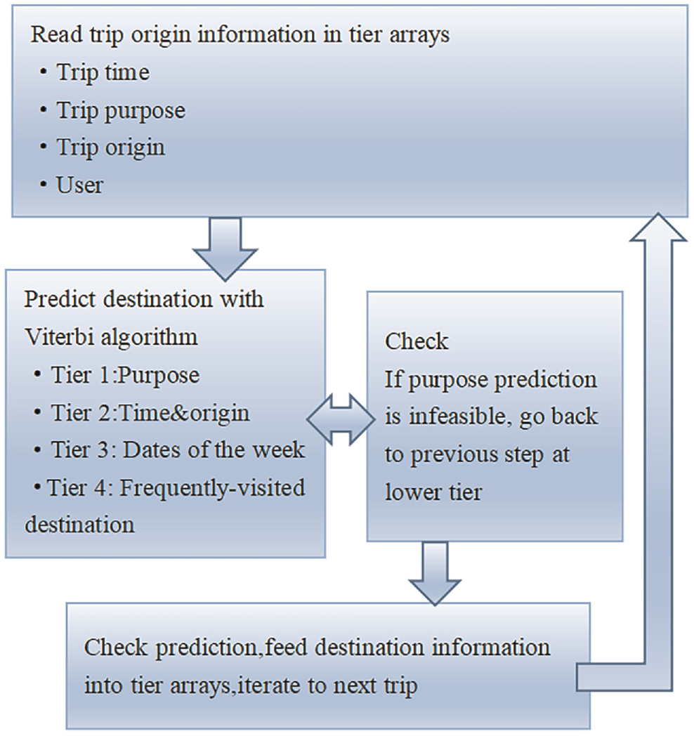
The hidden Markov model (HMM) algorithm process.
The prediction model starts by first reading the trip information from the user. This includes the latitude/longitude information of the origin of the trip, the identification tag of the user, and at what time the trip began. The whole process of destination prediction is completed before the trip. The model starts at Tier 1. A search is made for destination information from the same user and pulls the most common destination location that occurred from that trip purpose. In the process of HMM, Viterbi algorithm is used to predict the travel destination, which is used to find the most likely sequence of hidden states. If no estimation can be made, either because of lack of learned information from previous trips or because no one destination has a higher likelihood of occurring than any other destination, the model moves on to the next tier. At Tier 2, a search is done for all other previous trips that occurred at both the same hour of the day and the same origin as the current trip that it is being estimated. If there is information in this array, then the most common destination of the same origin and time of day are made similar to the previous tier. There is a chance that the destination prediction that has just been made is the same as the previous correct destination. This means that the script is probably incorrect, and the algorithm goes on to Tier 3. The same steps are then taken to make an estimation on simply the data of week, and the check occurs again to see if it must move on to Tier 4. At Tier 4, the algorithm has run out of possible searches and simply selects the most abundant location that has not yet been used from the previous three tiers. Once the estimation is made, the script checks whether it is correct, loads the information into the appropriate arrays for future estimation, and then moves onto the next trip. At no point can information from future trips be used, and past trip estimations are not changed after the algorithm has moved onto the next step.
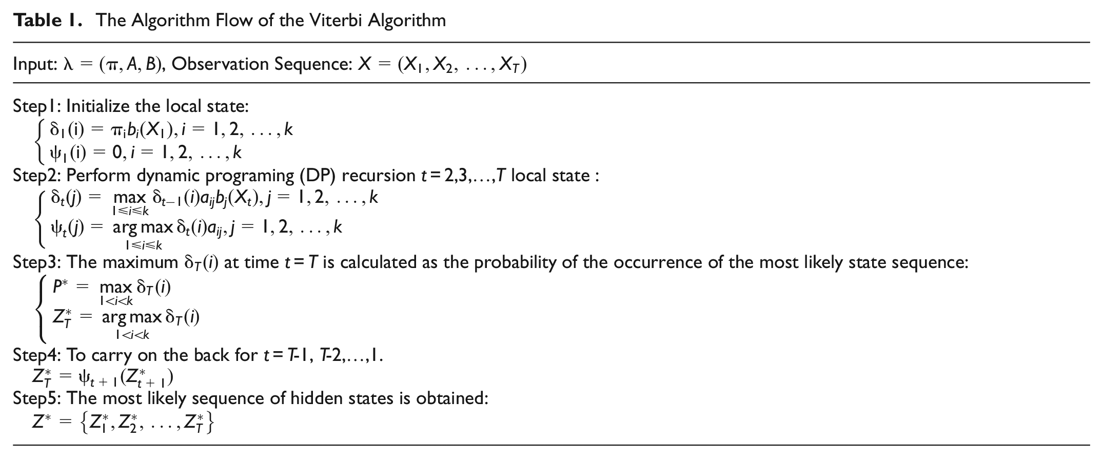
HMM is applied as it can help to obtain the most likely sequence of hidden states based on the sequence of the observations (
14
). The factors that formally define an HMM are
The Algorithm Flow of the Viterbi Algorithm
Model Calibration
The HMM is calibrated using multi-day GPS survey data from the first 4 weeks. The elements that formally define an HMM are
The Steps of Model Calibration
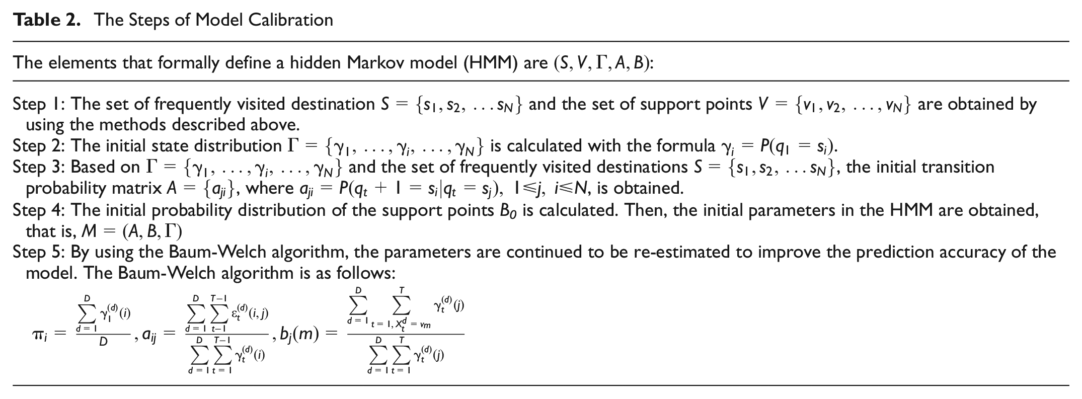
The new estimate Mn is considered to be a better estimate than the previous estimate Mp, if
Case Study
Beijing Yizhuang Economic Development Zone is the only national economic and technological development zone in Beijing. The research areas cover the core district, Ludong district, Hexi district, and Lunan district. Studying the travel behavior of the areas provides a value basis for the transportation development planning of emerging cities.
Data
In the process of travel behavior research of urban residents, 128 respondents were selected from different residential areas and participated in a consecutive 6 week travel survey in Yizhuang district, Beijing, in 2019. The first 4 weeks’ survey data were trained for modeling and the last 2 weeks’ data were employed in model testing. Each participant was required to complete a trip diary via an online survey, with which it was possible to conduct the testing and correction step for the trip identification results. A total of 128 questionnaires were sent out and 110 valid questionnaires were collected. The effective rate of questionnaires was 85.93%. Through analyzing the personal movement data collected by multi-day GPS, the movement patterns—the origin where a traveler usually departed from and the destination where a traveler usually went to—can be discovered.
There are several difficulties in the data prepossessing procedure ( 15 ). Firstly, participants submitted inaccurate or false travel information. Therefore, information in the survey data may not match the GPS data. To resolve this issue, one traveler’s travel rules were first ordered to process the survey data. After overcoming challenges, a total of 16,738 activities were obtained. For the raw survey data and GPS data, it is necessary to identify and remove random errors ( 16 ). The data preprocessing rules to process and remove invalid and inaccurate data are shown in the below:
Delete the travel times of each passenger if it is is zero or one time, which ensures that everyone has a normal travel data.
Exclude children less than 12 years old from the dataset.
Deleting the data of travel time less than 5 min and more than 2 h.
The GPS data with the time stamp greater than their next GPS point are identified and discarded.
After removing the unrealistic GPS points, the segments with the number of GPS points less than a threshold are identified and discarded.
Data Analyse
The survey data is used as source data to obtain the basic information which can be applied to the case study. The basic travel information includes the distribution of the activity duration and the distribution of the time when the activity occurs. The categories of the trip destination in this paper are “home,”“work,”“education,”“shopping,” and “other.” ( 17 ) Therefore, all the trips in the questionnaire are categorized into those groups.
Distribution of Activity Duration
People undertake different activities normally for different duration. Typically, there are some basic rules for some activities in relation to duration; work may take 4 to 8 h per day and education may take 3 to 6 h per day. The distributions of different activity duration (Figure 3) illustrates that work and education are more likely to occur when the duration is from 4 h to 10 h. Shopping mostly takes less than 3 h. Working dominates the activities when duration is longer than 8 h. Therefore, a rule is created to test the effect of activity duration on purpose imputation—if the duration is longer than 4 h and the purpose detected from GPS data is not work or education, this purpose should be suspected as being possibly wrong and the purpose may need to be redefined.
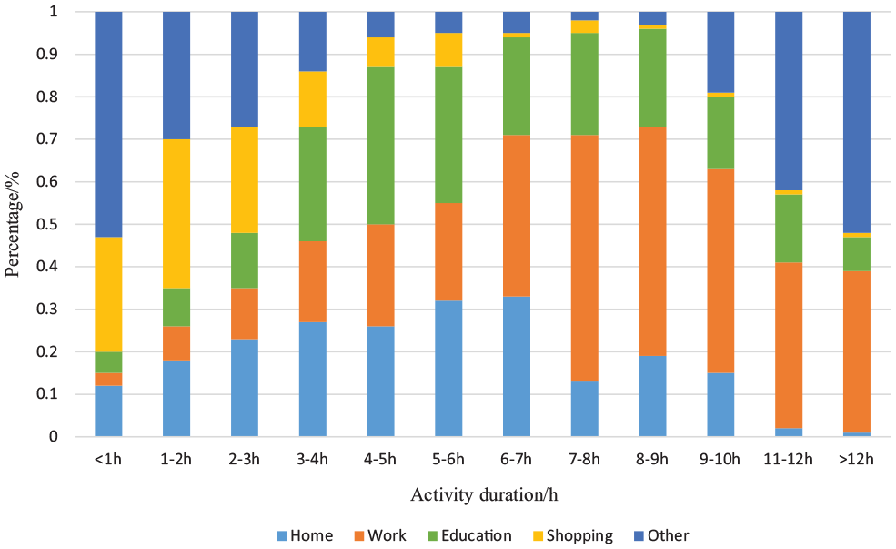
Distributions of different activity duration.
Distribution of the Time when Activities Occur
Similar to the activity duration, there are also some basic rules for the time when an activity occurs. Working trips are more likely to start from 8 to 9 a.m. and finish at 5 to 6 p.m. The hourly distribution of the time when activities occur (Figure 4) shows a 24 h distribution of the time when activities occur, and education rarely starts before 6 a.m. or after 9 p.m. Working is more likely to start in the morning, which is because people often go to work in the morning. In addition, combining with the activity duration figure, if duration is longer than 6 h and the activity occurs before 9 a.m., the trip for that activity is more likely to be work or education—addresses of work places and schools could be used to distinguish work and education trips.
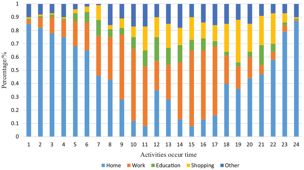
Hourly distribution of the time when activities occur.
Model Calibration Results
Implementing the Baum-Welch algorithm based on the sample data, estimates were obtained for the four parameter sets including the probabilities of initial state, the transition probabilities, and the mean and variance of every type of travel destination.
The first step is to investigate the transition matrix to show how the activity sequence for a trip chain is generated. The reason the transition probabilities are simple is that the lengths of the trip chains in the sample ranged from two to five, which is very short. The estimated transition patterns are so straightforward that such a complex methodology could be unnecessary. However, if longer trip chains are available from multi-day GPS data, the transition probability would provide in-depth understanding for use in composing the activity sequence for a trip chain. For example, when the current state is the trip destination of the “work” type, the next state is most likely to be a “home” type. An interesting finding is that the “work” type might switch to another the “home” type with a considerable degree of probability (0.108). This implies that trip chains other than piston trips of home-to-work-to-home, the length of which are longer than two, included consecutive flexible out-of-home activities.
The remaining parameters to be estimated for an HMM are the initial probabilities for choosing each activity. Since all trip chains in the sample are chosen such that they start with an overnight stay from the first day to the next day, only two activities are estimated to have an initial probability. While the typical home stay covers 58.3% of the initial state, it accommodates the remaining 41.7%.
The last step is intended to generate the most probable sequence of activities for a trip chain based on the parameters estimated above and on the observed feature vectors.
Results
Identifying Frequently Visited Destinations
Frequently visited destination refers to the trip destination of which the visiting frequency is not less than a certain value. This method for identification of trips and trip destinations proposed by Yan et al. is used in this paper ( 18 ). To prevent missing frequently visited destinations, 0.13 times and 0.28 times per day for weekdays and weekends, respectively, are defined as the visiting frequency threshold. That is, if the visit frequency of a trip destination is not less than 0.13 times and 0.28 times per day for weekdays and weekends, it can be taken as a frequently visited destination.
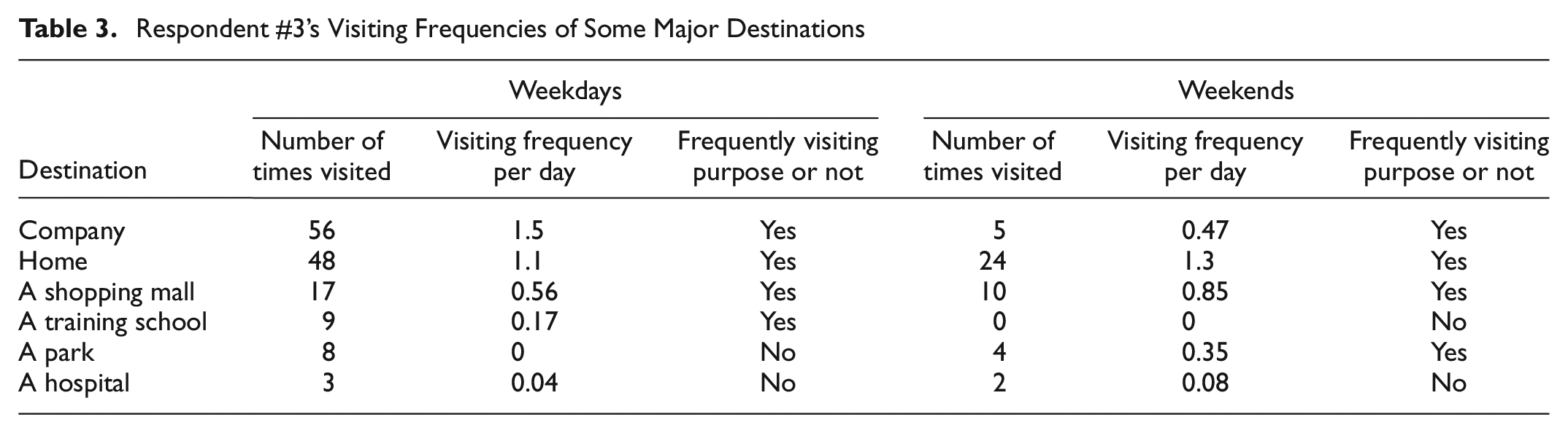
Respondent #3’s visiting frequencies (Table 3) for weekdays and weekends indicates that the frequently visited destinations are company, home, a shopping mall, and a training school on weekdays, while home and a shopping mall are the destinations being visited frequently on weekends. The statistical result of visiting frequency shows that the minimum value of visiting frequency is 0.17 times per day on weekdays, while the minimum value of visiting frequency is 0.35 times per day on weekends. This indicates again that the patterns of destination choice on weekdays and weekends are different from each other.
Respondent #3’s Visiting Frequencies of Some Major Destinations
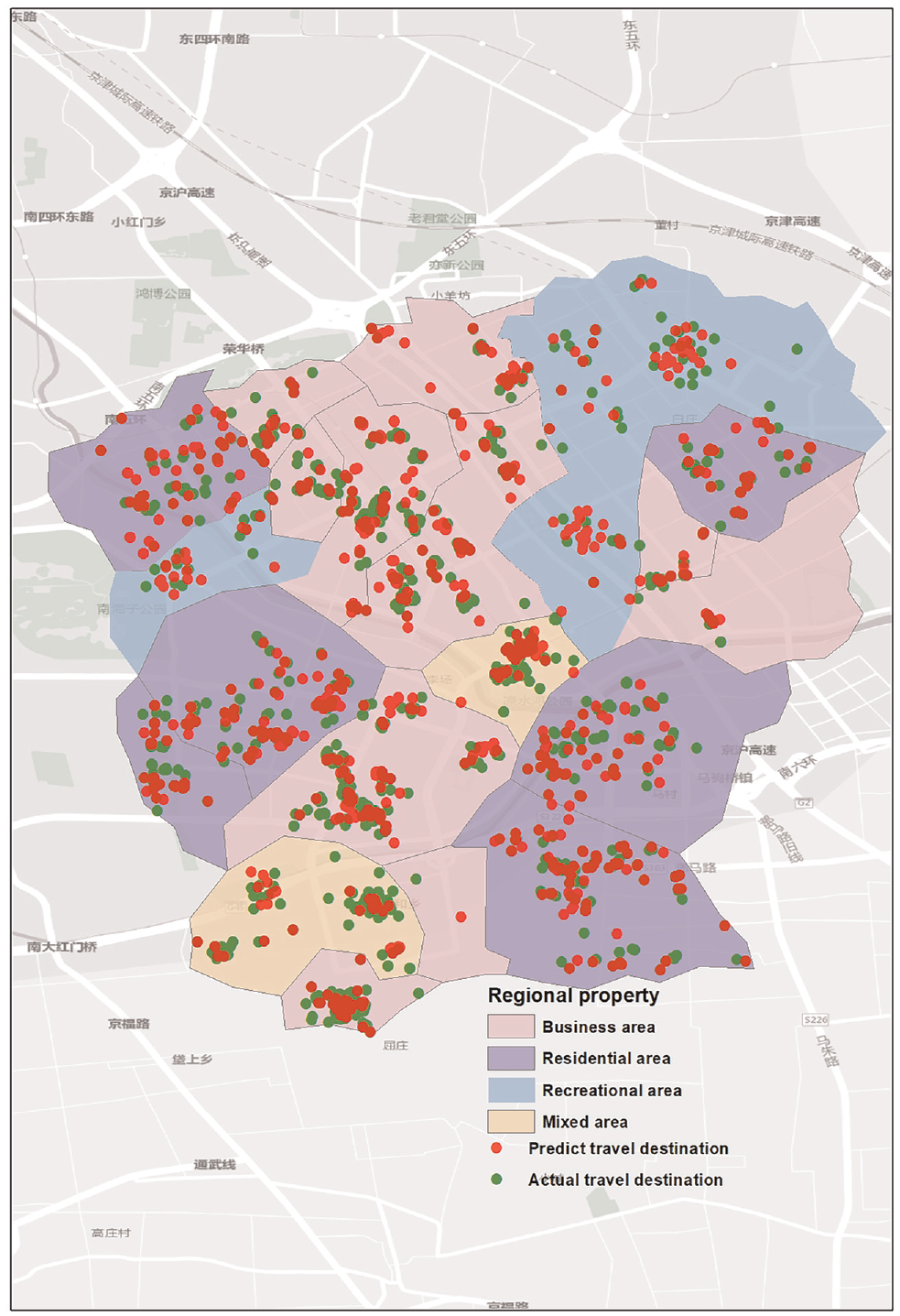
According to GPS travel data and travel destination data based on HMM, the actual travel destinations and forecast travel destinations distribution maps for weekdays and weekends (Figures 5 and 6) are obtained. The results show that the actual travel destinations in the commercial district and residential areas have high agreement, which is a result of the single travel purpose and the regularity of travel activities caused by daily commuting. In leisure and mixed areas, trip destinations are more concentrated on weekends than on weekdays. However, comparisons were made with commercial and residential areas and the two destinations matching error is bigger. This is because people’s leisure activities have greater instability; people will have different preferences for each restaurant and shopping mall—if they experience a bad restaurant, the next travel will change to other restaurants, leading to irregular travel destinations and forecast deviation.
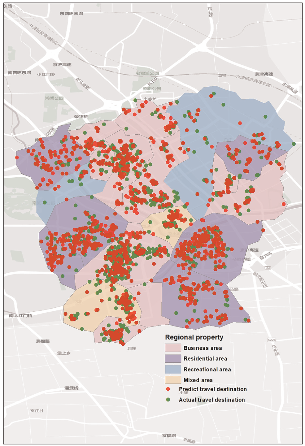
Actual travel destinations and predicted travel destinations distribution for weekdays.
Actual travel destinations and predicted travel destinations distribution for weekends.
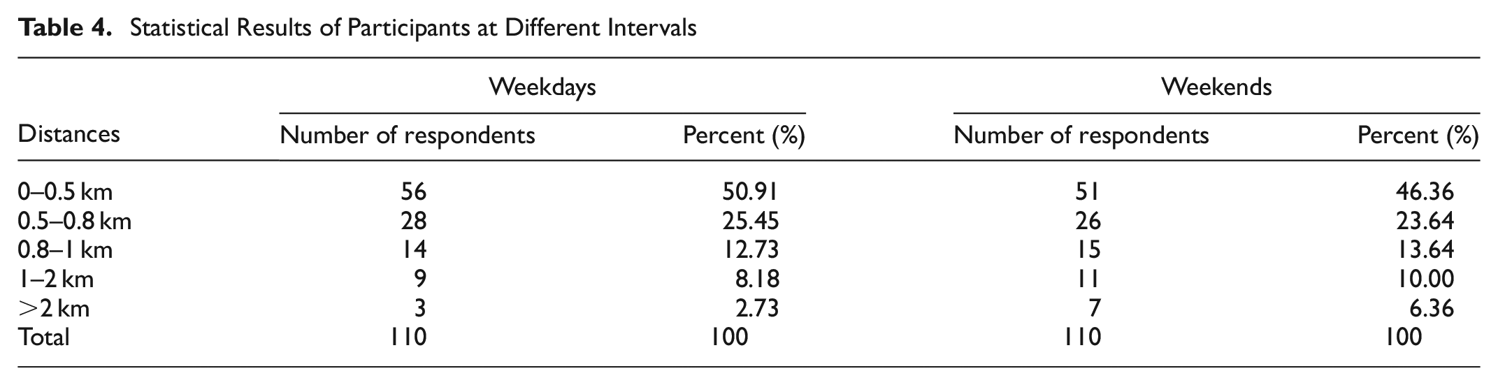
The distance threshold method is used to match the actual travel destination and predicted travel destination of travelers for weekdays and weekends, and calculate the proportion of participants in each interval. If the proportion of matches with small distances is greater, the prediction accuracy of travel destination is higher. The total proportion of the number of matches at different distances for weekdays and weekends (Table 4) is shown in the figure below. The distance between the actual travel destination and the predicted destination is less than 1 km as the limit of good prediction effect. The results show that the instances of the distance between the actual travel destination and the predicted travel destination being less than 1 km account for 89.09% and 83.64% for weekdays and weekends, respectively, which indicates that the HMM has a high accuracy of prediction.
Statistical Results of Participants at Different Intervals
Prediction Accuracy of Trip Destination
This section further compares the HMM with several state-of-the-art algorithms, including support vector machine (SVM), K-nearest neighbors (KNN), and RF. The core of the SVM model is to construct a “hyperplane” and use the hyperplane to divide different types of data. By optimizing SVM with a grid search method, the best C value, epsilon value, and gamma value in SVM regression are selected for trip destination prediction. KNN is the prediction of unknown category samples by searching the nearest k known category samples. The multiple cross validation method is used to determine the k value, and k = 5 is set after tuning. RF is a voting mechanism using multiple decision trees to solve classification or prediction problems. After tuning RF using the grid search method, the number of random samples as candidate variables is set to five. Finally, SVM, KNN, RF, and HMM are used to predict travel destinations for weekdays and weekends, and the prediction accuracy results of different models (Table 5) are obtained as follows.
Accuracy Comparisons of the Prediction of Trip Destination
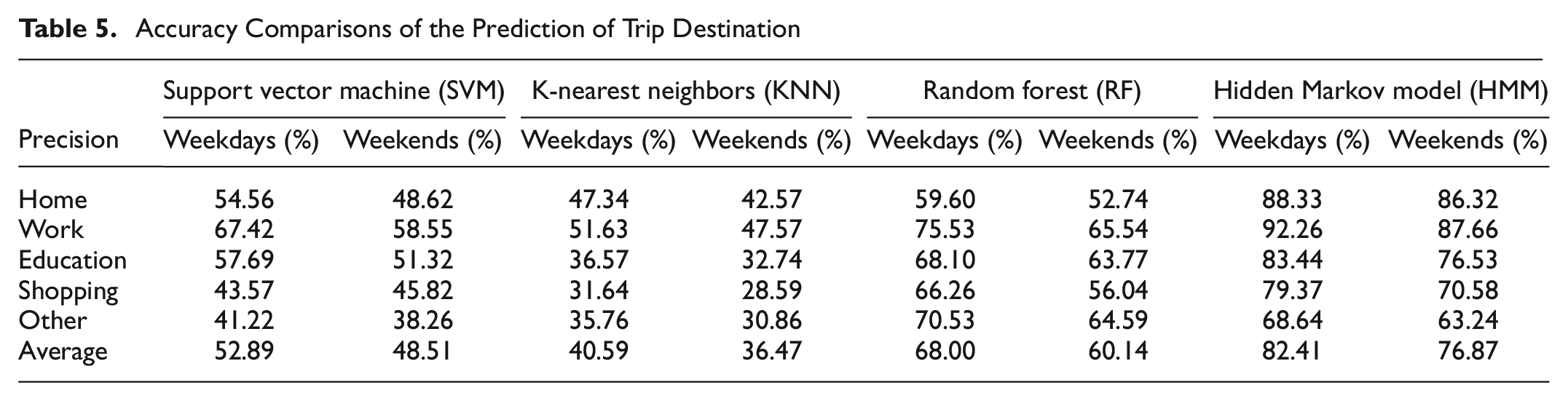
In Table 5, it can be observed that the HMM outperforms other algorithms on most trip destination categories in accuracy, and the prediction accuracy of travel destination on weekdays is generally higher than that on weekends. The accuracy of “home” and “work” decreased slightly over the weekend compared with weekdays, but overall showed the highest accuracy. This can be explained by the land use characteristics that help to identify these zones, providing increased information about the areas. Additionally, the accuracy of “education” is also high because it matches similar trips using land use types for government/public/services. Understandably, the prediction performance of “shopping” is relatively lower than “home,”“work,” and “education.” One important reason is that there are many functional areas. For example, a shopping mall or an office building contains multiple businesses and offices, including shopping, dining, and other functional areas. At this time, individuals can visit a place for a variety of activities. In this case, the destination of the trip is difficult to define. The accuracy of “other” is lower compared with other methods, and also is the lowest compared with other travel destinations, because people tend to classify an activity as “other” when it is difficult to separate it into another category. RF performs better in “other.” The underlying reason is that RF is such an ensemble learning method that it can achieve higher accuracy for complex classes, like “other.” Since RF performs especially well in this class, it can be employed for predicting “other” especially.
The prediction confusion matrices of HMM on weekdays and weekends (Figures 7 and 8) are illustrated as follows.
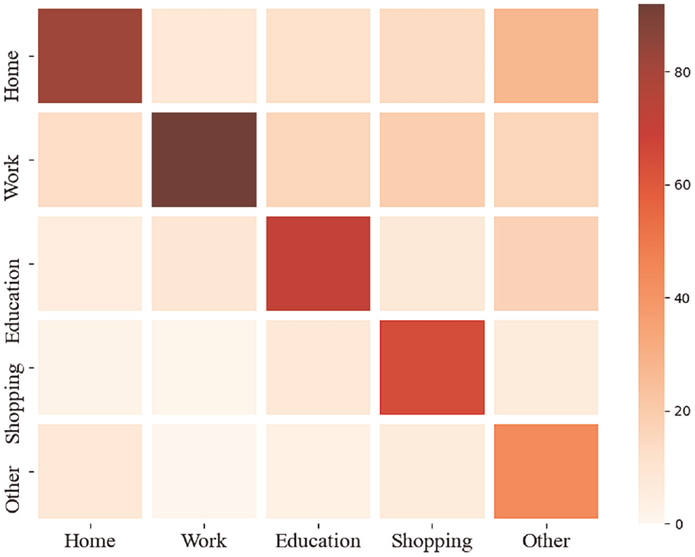
Prediction confusion matrix of the hidden Markov model (HMM) for weekdays.
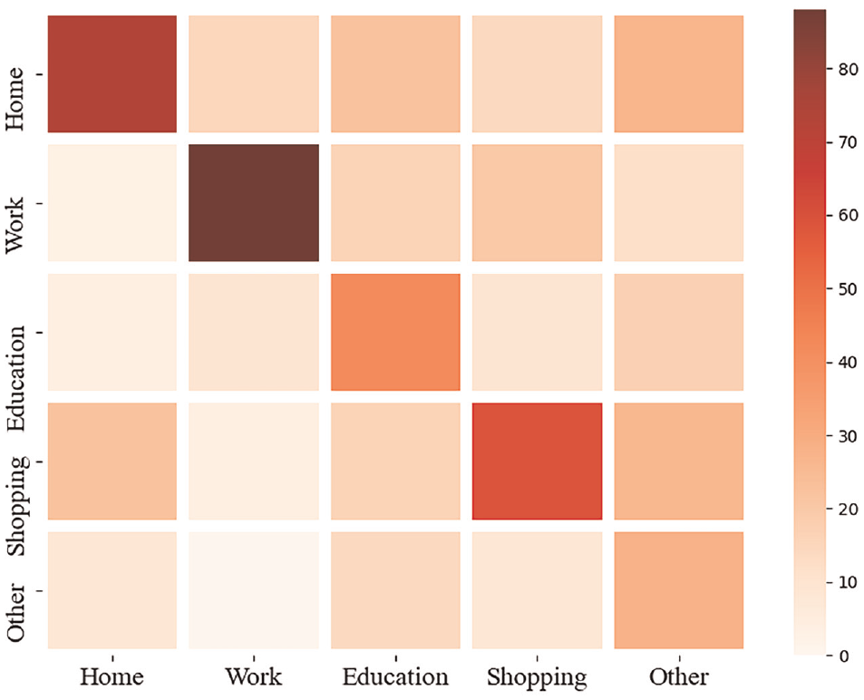
Prediction confusion matrix of the hidden Markov model (HMM) for weekends.
In general, HMM provides a better description of data and leads to better accuracy. Therefore, HMM scores the highest average accuracy. Moreover, HMM achieve extremely high performance for “work” activities, whereas other algorithms only reach low accuracy. As a result, HMM is very powerful in the prediction of trip destination on weekdays and weekends.
Conclusions and Discussion
In this article, an HMM for trip destination prediction with multi-day GPS data and survey data is developed. Both the trip destination models are calibrated by using the data on weekdays and weekends. Firstly, this paper identifies the frequently visited destinations with the time threshold of 4 min, taken as one of the predictor variables of the HMM. The results indicate that the average number of destinations for each traveler on weekdays and weekends is 11.58 and 8.47, respectively, and the patterns of destination choice on weekdays and weekends are different from each other. Secondly, this paper carries out data characteristic analysis, including the distribution of the activity duration and the distribution of the time when the activity occurs, and the two characteristics show that residents travel with obvious regularity. Thirdly, this study employs an HMM with Viterbi algorithm to predict the trip destination and with Baum-Welch algorithm to calibrate. By comparing the HMM with several state-of-the-art algorithms, the result is the HMM outperforms other prevailing algorithms. Fourthly, this research conducts the trip destination prediction for weekdays and weekends. In relation to frequently visited destinations identification and trip destination prediction, the prediction accuracy of the weekdays is always higher than that of the weekends, because people’s travel activities are more regular during the weekdays and the travel activities of the weekends are more flexible.
The model system proposed by this paper can be applied in trip destination prediction, which provides travelers, planners, or managers with destination prediction information before trips. Specifically, the trip forecasting results can be used in Automatic Terminal Information Service (ATIS) by revealing trip information, such as traffic conditions and commercial facilities around the destination. In addition, the trip prediction can be used in real-time travel navigation, providing travelers with route guidance and key facilities recommendation. It should also be pointed out that the methods provided in this paper can also be applied in destination prediction with the multi-day destination choice records collected from other data sources. Finally, the prediction of travel destinations is of great practical value in health and security fields such as epidemic prevention and control. A comprehensive understanding of the flow characteristics of individual travel and an accurate prediction of the travel location can play a positive role in the prevention and control of an epidemic.
One limitation of the current study is failing to take into account the possible factors that could affect trip destination choice, such as traffic conditions and some managing strategies like regional congestion charges. Therefore, the consideration of real-time traffic conditions and traffic management policies will be one of the research points for the following study. In addition to forecasting trip destination, it is also very important to predict travel route, in which the habit-related factors should also be considered. Besides, in the further study, attempts will be made to utilize the multi-day destination choice data collected in other cities to verify the results of this paper.
As a future research direction, using the available unlabeled GPS trajectories and leveraging the semi-supervised and unsupervised learning algorithms can be a potential compensation for not accessing a large labeled dataset. In addition to forecasting trip destination, it is also very important to predict travel route, in which the habit-related factors should also be considered. Besides, in the further study, attempts will be made to utilize the multi-day destination choice data collected in other cities to verify the results of this paper.
Footnotes
Author Contributions
The authors confirm contribution to the paper as follows: study conception and design: Z. Jin, Y. Chen; data collection: Y. Chen, C. Li; analysis and interpretation of results: Z. Jin, Z. Jin; draft manuscript preparation: Z. Jin, C. Li, Z. Jin. All authors reviewed the results and approved the final version of the manuscript.
Declaration of Conflicting Interests
The author(s) declared no potential conflicts of interest with respect to the research, authorship, and/or publication of this article.
Funding
The author(s) received no financial support for the research, authorship, and/or publication of this article.