Understanding Productivity in the Transportation Construction Industry

Abstract

There is an ongoing long-term debate about trends in construction productivity. This research examines the productivity of the transportation construction segment, specifically the transportation construction industry in Colorado. The paper examines 14 years of transportation data from 880 projects executed in the state of Colorado between 2004 and 2016. By evaluating the coefficients extracted from over 35 linear regression models, it analyzes how productivity in the Colorado transportation construction industry has evolved over recent years. Provided with a rich database, the study focuses on productivity at the more detailed project level, which will help explain the varying trends observed by different authors. This level of detail presents a comprehensive analysis of productivity for a segment of the transportation construction industry that has not yet been described in the literature.

Keywords

infrastructure construction construction management scheduling project delivery methods general performance and performance tests highway maintenance maintenance and operations management highways maintenance

Understanding how construction productivity behaves has been a topic of debate for at least two decades. This debate is not unjustified, because understanding productivity and what drives it could potentially lead to leaner, more efficient, and better highway construction projects. The two main perspectives with regard to productivity trends are whether there has been a decline or an increase in productivity in the transportation construction industry. Transportation construction spending exceeds US$40 billion annually ( 1 ), and this justifies a closer examination of what has been occurring in the sector in relation to productivity. The amount of industry spending is interesting, because overall construction industry expenditure has been fluctuating since 2004 (Figure 1), showing a big decline during the last recession (2007–2009) and a steady increase after that. On the other hand, not only has expenditure in the transportation construction sector specifically been increasing since 2004, it has also increased its percentage of overall construction industry expenditure (Figure 2). These facts reiterate the importance of understanding how productivity is behaving, so the industry can focus on adjusting its efforts accordingly.

Figure 1.

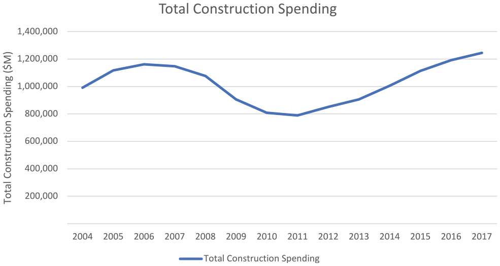
Total construction spending ( 1 ).

Figure 2.

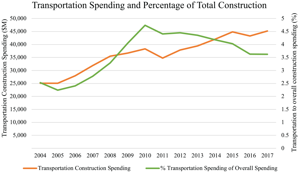
Transportation construction spending and percentage of transportation spending versus overall construction spending ( 1 ).

Some researchers have pointed out that productivity in transportation construction has stagnated, or is even declining ( 2 ). Teicholz ( 3 ) suggests some of the causes for this behavior. First, the uniqueness of individual construction projects makes it difficult to overcome the learning curve of executing the projects, because it is unlikely that any two will be the same. Second, because small firms conduct a lot of the business, and it is difficult for smaller firms (<5 employees) to make investments in newer technologies or methods, it is hard for them to adapt to the industry. This means that roughly 70% of construction firms have a big turnover of labor. Third, declining real labor prices can lead to a decrease in investment in prefabrication and equipment, which reduces productivity. In addition, lower labor prices can result in firms hiring unskilled labor (generally, less productive than skilled labor), which can result in worse productivity. Fourth, a competitive—rather than collaborative—procurement system reduces the collaboration between parties involved in projects. This creates a risk-averse environment for construction projects. With a risk-averse approach, parties protect themselves from other players’ errors, leading to over-budgeted projects with more claims, which, subsequently, cause delays and reduce productivity.

Further, Sveikauskas et al. ( 4 ) suggest that productivity has increased in the construction industry in three out of four sectors: single-family housing; multiple-family housing and commercial construction. However, their research suggests that productivity in the transportation construction industry (roads, bridges, and highways) has been declining. Sveikauskas et al. ( 2 ) used a standard method to measure productivity by creating a ratio of real output (work installed) to input (labor hour) ( 5 ). Then, the calculated yearly ratios were compared with other years to observe whether there was a decrease or increase in the productivity trends. The use of the ratio allowed them to compare productivity on a yearly basis, contrary to the usual method of comparing the beginning and end years of a certain period. Their research does point out that construction productivity, even when showing increasing trends, is not increasing as much as in other industries, such as manufacturing. Like Sveikauskas et al.’s study ( 2 ), the current research will also analyze productivity trends on a year-to-year basis but will be specific to the transportation construction industry. In addition, it will compare productivity at the project level.

Even when there is a lack of agreement about how productivity is behaving, there seems to be a consensus that measuring it is a challenge. Some of these challenges have been highlighted by previous research efforts. Goodrum et al. ( 6 ) concluded that productivity has been increasing at the activity level. However, they highlight that this increase in productivity is not revealed when trying to explain productivity at the industry level.

There are a lot of challenges when measuring productivity at the industry level. One of the biggest is finding accurate and reliable deflators to measure construction real output ( 2 ). A deflator is a metric used to measure the changes in the value of prices through time ( 7 ). The deflator used for the highway construction industry is the National Highway Construction Cost Index (NHCCI). Even though according to the definition provided by the Federal Highway Administration (FHWA) the index is called a cost index, the NHCCI is actually a price index ( 8 ). One advantage of using a price index as opposed to a cost index is that the latter assumes a constant relationship between inputs and outputs. This means cost indexes assume that productivity remains unchanged over time. Most cost indexes also fail to consider the profit contractors obtain per item, that is, they use list prices rather than actual costs ( 9 ). The deflator used in this research, the NHCCI, measures the average change in price of items across the industry. To do so, winning bids are used to extract the pay items (comprised of labor, materials, and/or services). These pay items are then averaged to create a mean value across the whole industry. The NHCCI was revised and updated in 2017 by comparing it with the Producer Price Index (PPI), and it is now more adjusted to the reality represented by the PPI.

The importance of using a good deflator is often highlighted by other researchers. For example, for the period between 1968 and 1978, it is estimated that over 50% of the decline in construction productivity could be attributed to overdeflation, in other words, using poor deflators ( 10 ). Anther cause of poor deflation is using proxy indexes, which are indexes used to deflate an industry when it lacks its own index (e.g., using a single-family house index for commercial construction) ( 9 ). Because FHWA has its own deflator (NHCCI), this increases the reliability of the deflated values. Allmon et al. ( 11 ) also highlighted the importance of selecting a good deflator when comparing historical productivity trends. In addition, they emphasized the disadvantage of using cost indices is that they assume constant productivity.

Additionally, there is a lot discrepancy with regard to how to measure aggregate data outputs. Furthermore, uniformity in the measurements of productivity cannot be assumed ( 6 , 12 ). These two statements were validated when Vereen et al. ( 13 ) proved that even when using the same projects, productivity could show varying trends. This variation was attributed to the way output data were measured. The authors measured productivity using the same data, but computed output data in four different ways, which produced four different productivity trends. The difference found in the trends was such that some showed an increase in productivity whereas others showed a decrease. Again, the trends were computed using the same data.

The current research aims to conduct a more detailed analysis of productivity trends within the transportation construction industry. It also aims to validate some of the most recent findings (Sveikauskas et al. [2, 4]). Sveikauskas et al. ( 2 ) found there has been a lack of accuracy in industry-specific productivity studies because of the unavailability of industry-specific deflators. However, this has changed over recent years, so research conducted during the last few years has been using more robust and consistent data. Analysis and validation of the current research has been conducted using data from the transportation construction industry, specifically, from projects executed in Colorado between 2004 and 2016. Potentially, the analyses conducted in this research will also help to measure productivity trends in the future. Because the current research analyzed transportation construction projects executed in the state of Colorado between 2004 and 2016, it is important to highlight that the quantity of work installed (adjusted for inflation to 2003 US$) indicates an incremental trend (Figure 3) similar to the one shown at the federal level in Figure 2.

Figure 3.

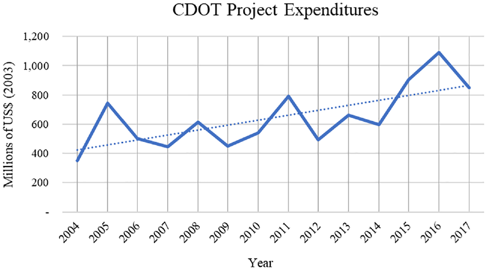
CDOT total construction work installed (adjusted for inflation to 2003 US$).

Research Methodology

This section describes the data used to conduct the statistical analyses, and the two steps of the methodology. This research used real output (US$ deflated to 2003) and input (work days) to measure productivity, which are X and Y in the regression models, respectively.

Description of the Data

This research used production data from over 880 transportation projects executed in Colorado between 2004 and 2016. The data include project cost, project type, year of project execution, and project duration in work days, which is measured in charge days, that is, the days on which work was actually being carried out and does not include weather delays or holidays. However, because the intention was to analyze the project types and years independently, the research ran a regression for each project type and year combination, so only two variables will be involved in the regression models:

durations, measured in work days, (dependent variable Y), which describes the number of charge days required to complete the projects; and

work installed, measured as the total cost deflated to 2003 US$ using the NHCCI (independent variable X).

The data provided by the Colorado Department of Transportation (CDOT) consisted of 896 projects ranging from $67,462 to $62,750,652 with a mean of $5,035,362 (2003 US$).

Because the visual assessment conducted for the data showed they were nonnormal, they were transformed using logarithmic transformations before conducting any analyses. The linear regression assessments are described in the next section of the paper. Additionally, normality tests were conducted, and concluded that durations and work installed are not normally distributed.

The normality test results for the charge days and durations are shown in Table 1.

Table 1.

Test for Normality of Charge Days and Durations

Variable	n	Skewness	p-value (skewness)	Kurtosis	p-value (kurtosis)
Work installed	896	4.075	0	33.25	0
Durations	896	2.69	0	10.62	0

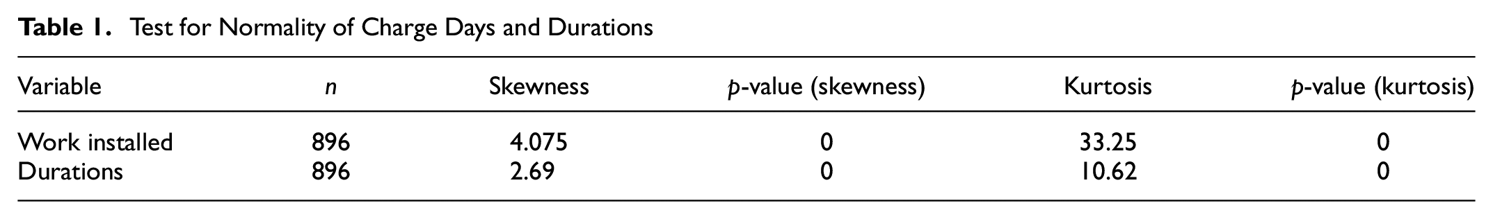
The results show that both work installed and durations failed the normality tests.

Data Analysis

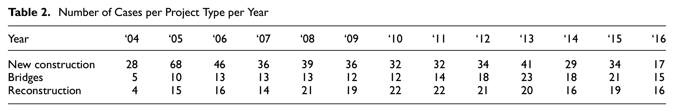
To measure productivity, the current research analyzed the coefficients from 37 different simple linear regression (SLR) models. Table 2 shows the number of cases per project type, which is important, because a minimum number of projects is required per predictor variable. According to Fisher’s generalization, the aforementioned minimum should follow the rule n/k > 10, where n is the number of cases and k the number of predictors ( 14 , 15 ). Therefore, the two analyses for 2004 where n ≥ 10 were not conducted.

Table 2.

Number of Cases per Project Type per Year

Year	‘04	‘05	‘06	‘07	‘08	‘09	‘10	‘11	‘12	‘13	‘14	‘15	‘16
New construction	28	68	46	36	39	36	32	32	34	41	29	34	17
Bridges	5	10	13	13	13	12	12	14	18	23	18	21	15
Reconstruction	4	15	16	14	21	19	22	22	21	20	16	19	16

Creating First Set of Regressions

The first step consisted of creating SLR models for three major project types: new construction (roads and highways); reconstruction (roads and highways); and bridges. For each project type, the research created one regression per year, and extracted the regression coefficients. The regression coefficients represent the change in duration of a project per quantity of work installed. Accordingly, a large coefficient means that more time is needed to execute a project, compared with a smaller coefficient. In other words, the value of a dependent variable (durations) can be estimated using a constant value plus the product of the slope and the independent variable (work installed), and an error term:

\hat{Y} = β_{0} + β_{1} X + \in

(1)

where

$\hat{Y}$ is the predicted value of Y (duration),

$β_{0}$ is the intercept,

X is the independent variable work installed,

$β_{1}$ is the slope, and

$\in is$ the error term.

After obtaining the coefficients for each regression, the research proceeded to construct a new dataset, which contains two different types of variable: year, which indicates the year of the individual regressions; and work installed, which represents the coefficients of each regression model. This dataset is summarized in Table 3.

Table 3.

Dataset of Coefficients per Year and Work Installed

Year	Work installed (new construction)	Work installed (reconstruction)	Work installed (bridges)
2004	0.7	NA	NA
2005	0.67	0.55	0.73
2006	0.6	0.52	0.75
2007	1.09	0.7	0.86
2008	0.34	0.61	0.72
2009	0.4	0.46	0.55
2010	0.52	0.52	0.55
2011	0.73	0.41	0.67
2012	0.61	0.58	0.66
2013	0.58	0.67	0.64
2014	0.42	0.56	0.6
2015	0.79	0.56	0.5
2016	0.39	0.49	0.65

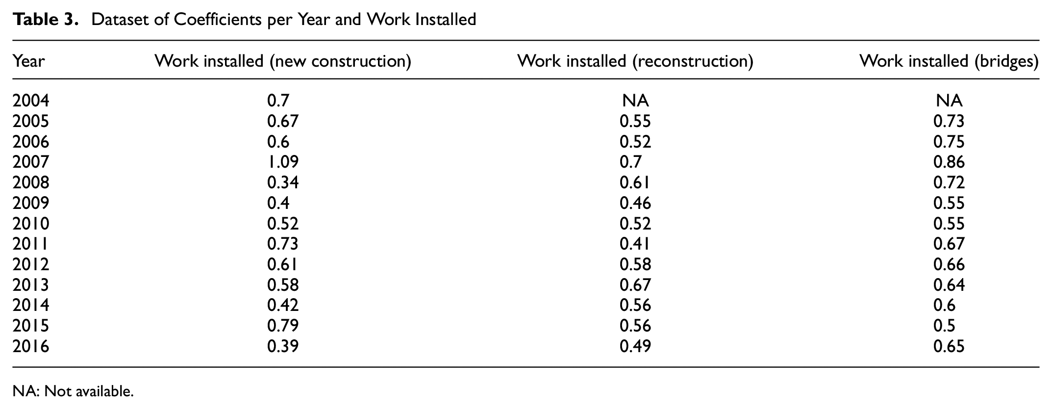
NA: Not available.

Creating Second Set of Regressions

Once the new dataset had been constructed, three different regressions were made, where the coefficients of work installed, or labor productivity coefficients from this point forward, (dependent variable) were regressed against year (independent variable). This process created three different and independent SLR models. Once the SLR models had been created, the regression equations were evaluated to study the slope (productivity trend) and test its significance. This process allowed us to evaluate the productivity trends from 2004 until 2016. The relationships between the labor productivity coefficients obtained from the SLR models across the specified period of time reveal the trend of productivity for the three major project types studied. Specifically, the change in the labor productivity coefficients represents a change in the impact of year with regard to the time required to install the quantity of work. In other words, if the labor productivity coefficients decrease over the years (indicating a negative slope), the productivity increases. The analysis conducted provides an easy and reliable explanation of how the productivity in the transportation construction sector has behaved over recent years.

The explanation of productivity using this SLR approach is done by creating a SLR equation. SLR takes place when the relationship between two variables approximates a linear function (equation [2]) ( 16 ). In other words, the value of a dependent variable (labor productivity coefficients) can be estimated using a constant value, the product of the slope and the independent variable (year), and an error term.

\hat{Y} = β_{0} + β_{1} X + \in

(2)

where

$\hat{Y}$ is the predicted value of Y (coefficient of work installed),

$β_{0}$ is the intercept,

X is the independent variable year,

$β_{1}$ is the slope, and

$\in is$ the error term.

After creating the regression models, the research analyzed how the labor productivity coefficients changed over time. This analysis provided an explanation of how productivity behaved over the observed 13-year period. The labor productivity coefficients derived from the regression are inversely related to the productivity trends. That is, if the labor productivity coefficients from the regressions are decreasing, it means that productivity has been increasing and vice versa. The reason for the inverse relationship is that the labor productivity coefficients (slopes) indicate how much the duration of a project changes with a change in the real output of a project. This means that with a smaller regression coefficient more work installed is required to increase the duration of a project by some magnitude, compared with a regression with a larger coefficient.

Linear Regression Assessments

To conduct linear regression analysis, the data have to meet certain criteria or assumptions as described below.

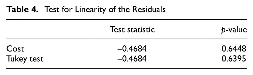
a. Linearity of the residuals

This assessment was conducted by running a residual test for the different models for each project type. Because the p-values were not significant, the residuals present a linear relationship. For demonstration purposes, Table 4 shows the output of the tests conducted to assess the linearity of the model used for bridges in 2010.

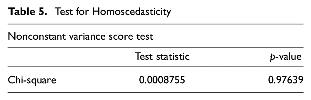
b. Homoscedasticity

This assessment was conducted to determine whether the values of the residuals have equal variance at different levels of work installed. A nonconstant variance test was conducted for each of the regression models, demonstrating that the assumption of homoscedasticity was satisfied. Table 5 shows a sample of the tests conducted.

c. Normality of the residuals

Because the regressions differ in sample size, the normality assessment differs. For those regressions with n > 25, the p-values observed were associated with skewness and kurtosis. Alternatively, for the smaller sample sizes, the p-values observed correspond to the Anderson–Darling (AD) and Shapiro–Wilk (SW) tests, respectively. For demonstration purposes, Table 6 shows one sample normality assessment for a regression with n < 25. The p-values of the AD and SW tests show that the residuals are normally distributed.

d. Independence of errors

To assess the independence of errors, a Durbin–Watson (DW) test was conducted to determine whether the residuals showed autocorrelation. Table 7 shows a sample DW test and it indicates the residuals are not autocorrelated.

Table 4.

Test for Linearity of the Residuals

	Test statistic	p-value
Cost	–0.4684	0.6448
Tukey test	–0.4684	0.6395

Table 5.

Test for Homoscedasticity

Nonconstant variance score test
	Test statistic	p-value
Chi-square	0.0008755	0.97639

Table 6.

Test for Normality of the Residuals

Residuals	n	AD test	AD p-value	SW test	SW p-value
Pearson	22	0.4139487	0.3361982	0.9559292	0.4116121
Standardized	22	0.4084187	0.3464158	0.9606144	0.5017999
Studentized	22	0.5387357	0.1672817	0.9391418	0.1900161

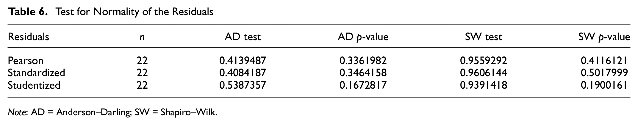
Note: AD = Anderson–Darling; SW = Shapiro–Wilk.

Table 7.

Test for Independence of Errors

Lag	Autocorrelation	DW test	p-value
1	0.3612578	1.276919	0.066
2	0.216036	1.56417	0.376
3	-0.2912191	2.511125	0.1
4	-0.2088289	2.281392	0.178

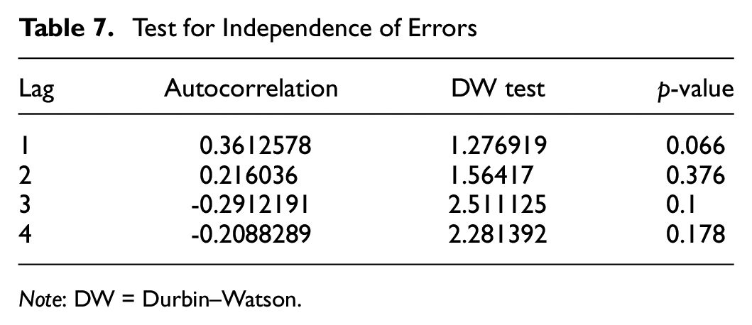
Note: DW = Durbin–Watson.

Interpreting the Labor Productivity Coefficients

For the data being analyzed in the current research, Y is the duration of projects and X is the quantity of work installed in relation to the projects. The quantity of work installed is measured in US$, converted to 2003 US$ to control for inflation. Controlling for inflation is a way of measuring real output or estimating the quantity of work installed ( 6 ). Additionally, the focus of this analysis is on the labor productivity coefficients (slopes) obtained from each regression equation. These labor productivity coefficients represent the slope of the linear relationships. In other words, they show how much the duration of projects changes with changes in the quantity of work installed. As mentioned earlier, the relationship between the labor productivity coefficients of work installed and productivity are inversely related. That is, smaller labor productivity coefficients mean that with more work installed the duration is smaller, compared with an equation with a higher coefficient. Put in simpler terms, smaller regression labor productivity coefficients mean better productivity and vice versa.

Analysis of Productivity per Project Type

This section describes how the labor productivity coefficients of the regression models vary from year to year for each of the selected project types. As described previously, each project type has one regression per year and the coefficient of each regression is then extracted and analyzed along with the other labor productivity coefficients for each of the years.

New Construction

Included in this category are road and road transportation construction projects that are not resurfacing, reconstruction, restoration, rehabilitation, or bridges. The labor productivity coefficients for work installed for each of the regressions are shown in Table 8 and graphically in Figure 4.

Table 8.

Labor Productivity Coefficients per Project Type per Year

Project type		2004	2005	2006	2007	2008	2009	2010	2011	2012	2013	2014	2015	2016
New construction	Intercept	–4.4	–4.0	–3.3	–9.5	–0.0	–0.7	–2.1	–4.9	–3.5	–3.1	−0.9	–5.9	–0.4
New construction	Labor productivity coefficient	0.70	0.67	0.6	1.09	0.34	0.4	0.52	0.73	0.61	0.58	0.42	0.79	0.39
Reconstruction	Intercept	–2.01	–1.51	–4.44	–2.95	–1.10	–1.50	0.08	–2.42	–3.69	–2.27	–2.26	–1.19	–2.01
Reconstruction	Labor productivity coefficient	0.55	0.52	0.70	0.61	0.46	0.52	0.41	0.58	0.67	0.56	0.56	0.49	0.55
Bridges	Intercept	NA	–3.93	–4.36	–5.26	–4.04	–1.73	–2.01	–3.34	–3.36	–3.01	–2.76	–1.27	–3.37
Bridges	Labor productivity coefficient	NA	0.73	0.75	0.86	0.72	0.55	0.55	0.67	0.66	0.64	0.60	0.50	0.65

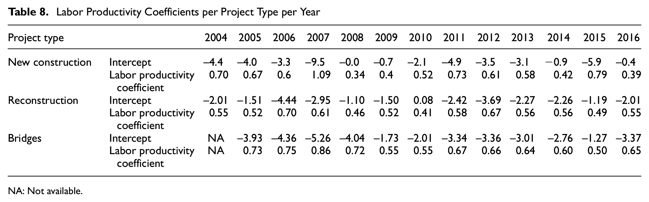
NA: Not available.

Figure 4.

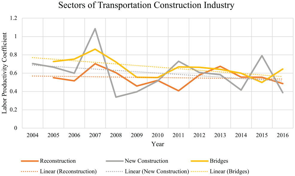
Derivation of the labor productivity coefficients—reconstruction, new construction, and bridges.

Reconstruction

Included in this category are road and road transportation construction projects that are described as rehabilitation, resurfacing, or reconstruction. These projects do not include bridges. The labor productivity coefficients for work installed for each of the regressions are shown in Table 8 and graphically in Figure 4.

Bridges

Included in this category are road transportation construction projects that involve rehabilitation, new construction, or reconstruction of bridges. The labor productivity coefficients for work installed for each of the regressions are shown in Table 8 and graphically in Figure 4.

The labor productivity coefficients shown in Table 8 were regressed on the variable year in three separate regressions. These results are shown in Table 9. In Table 9, the labor productivity coefficient for each of the project types represents the slope (i.e., productivity trend) for each of the project types over time. However, these results need to be validated with the p-value to determine whether they are significant. Table 9 shows the only significant trend observed was for bridges.

Table 9.

Analysis of Significance of Slopes

		Labor productivity coefficients	SE	t-value	p-value
New construction	(Intercept)	0.7031	0.12054	5.833	0.000114
New construction	Year	–0.01454	0.01519	–0.957	0.358917
Reconstruction	(Intercept)	0.569286	0.053809	10.58	9.46E-07
Reconstruction	Year	–0.002748	0.007311	–0.376	0.715
Bridges	(Intercept)	0.770335	0.050528	15.246	2.99E-08
Bridges	Year	–0.01739	0.006865	–2.533	0.0297

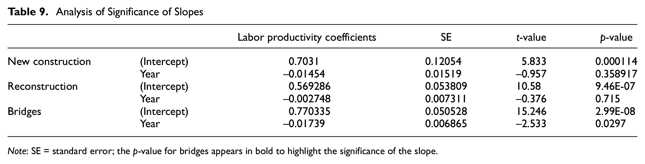
Note: SE = standard error; the p-value for bridges appears in bold to highlight the significance of the slope.

The results in Table 9 show that the negative trend of the labor productivity coefficients for bridges is statistically significant (meaning an increase in productivity). However, for new construction and reconstruction, it can be concluded that there was no statistically observed change.

Additionally, the coefficient derived from the second regression of bridge projects can be interpreted as a 2.64% increase in the productivity of this type of project, which was calculated as follows:

Extracting the average of the labor productivity coefficients from the first set of regressions. These regressions were developed using log-log transformed data, so the interpretation of their labor productivity coefficients is explained as 1% change of Y per $β %$ change of X (equation [3]):

% Δ Y = β_{1} % Δ X

(3)

2. Extracting the slope of the second set of regressions. These regressions did not transform the data, so the interpretation of labor productivity coefficients represents the amount of change in Y per a one-unit increase in X (equation [4]):

Δ Y = β_{1} Δ X

(4)

3. Finally, the percentage that $β_{1}$ from equation (4) represents in the average of $β_{1}$ from equation (3) is the annual percentage change in productivity over the period studied. However, because the changes in the labor productivity coefficients are inversely proportional to the productivity trends, a negative value represents an increase in productivity.

After extracting the labor productivity coefficients from equations (3) and (4) for bridge projects, we can conclude that there was a 2.64% increase in productivity between 2004 and 2016 for bridge projects executed in the state of Colorado.

Conclusion and Discussion

The findings of the current paper show that the trends in productivity for bridge projects demonstrated an increase from 2004 to 2016. However, this cannot be generalized to the whole transportation construction industry because although the productivity trends of new construction and reconstruction were moving in the right direction, they were not strong enough to show statistically significant results; it should be remembered that these data were only from Colorado. Based on the results obtained, the researchers can speculate as to why bridge projects was the only project type to show a reliable increase in productivity. First, bridge projects are likely to use prefabricated and modular elements, which increases efficiency ( 17 ), whereas this is very unlikely to happen in projects that do not involve bridges. However little research has been conducted to explore the productivity of transportation construction and even less for bridges ( 18 ). Thus, further research is needed to determine the contributions to the difference in productivity trends to validate this speculation.

Another condition worth considering is that, most—if not all—of the reconstruction projects have to deal with traffic and partial road closures. This can also be a reality for new construction, because if these projects involve expansion or widening, they can be carried out on existing roadways. Road closures and the traffic management involved potentially affect the shifts worked, because in congested areas it is challenging to close a road completely when carrying out work. Thus, nonconventional work shifts can be the result, and these can be more costly for the project (e.g., night shifts) ( 19 ). Because labor represents a significant proportion of a project’s cost ( 20 ), an increase in labor costs can have a negative effect on productivity—as measured in the current research (cost versus work days). Alternatively, bridge projects often involve full road closures, which allow the crews to work uninterrupted and alleviate the effect of traffic and nonconventional shifts.

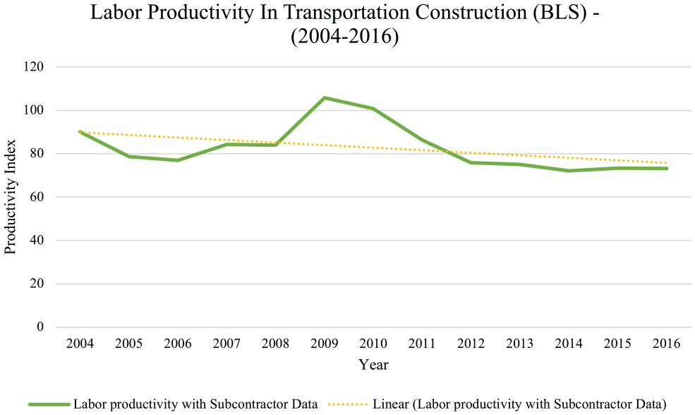
To some extent, the findings from the current research overlap with the findings of Sveikauskas et al. ( 2 ), who developed productivity indexes for four industries within construction. The current research only focused on the transportation construction industry in the state of Colorado. Sveikauskas et al. ( 2 ) developed a productivity index that used data from the Census of Construction (COC) as a gross output metric, which helped analyze the industry overall. With this metric, Sveikauskas et al. ( 2 ) finally developed a productivity index. However, because the data from COC do not include subcontractor data, Sveikauskas et al. ( 2 ) also developed a factor to account for subcontractors. Once this was achieved, they developed an index for the transportation industry that adjusted productivity to allow for the presence of subcontractors. Figure 5 shows a graphical representation of the indexes for the period 2002 to 2016. The conclusion from said study is that there was a yearly decline of 2.2% in transportation construction productivity for the period under investigation (2002–2016) ( 2 ).

Figure 5.

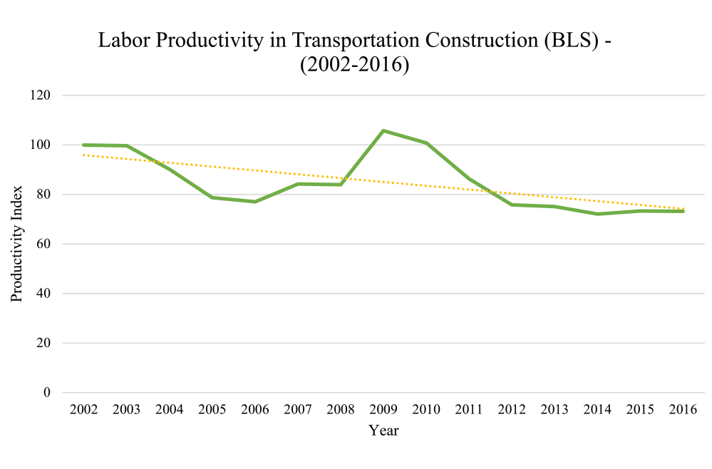
Productivity trends—BLS report (2002–2016).

Table 10 shows the slopes for the indexes (with and without subcontractor data) developed by Sveikauskas et al. ( 2 ) for the period 2002 to 2016. The table shows a significant decrease for the slopes at α = 0.05.

Table 10.

Analysis of Significance of Slopes—BLS report (2002–2016)

		Estimate	SE	t-value	p-value
Labor productivity	(Intercept)	97.4344	5.2438	18.581	9.59E-11
Labor productivity	year	–1.5472	0.5767	–2.683	0.0188

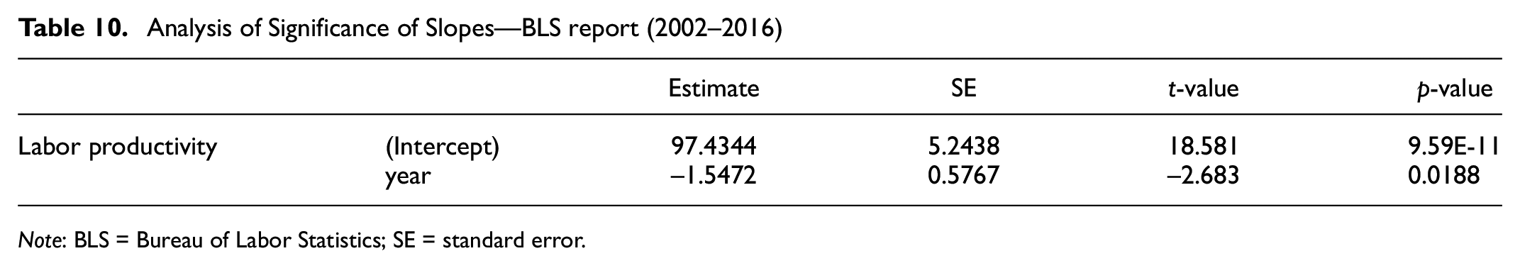
Note: BLS = Bureau of Labor Statistics; SE = standard error.

However, if the results obtained from Sveikauskas et al. ( 2 ) are analyzed for the same period studied in the current research (2004–2016), the slopes are not significant (Figure 6 and Table 10), which is also the case for the data analyzed in the current research (Figure 7 and Table 11). When the slopes are not significant, the only conclusion that can be drawn is that the productivity in the transportation construction industry did not change for the period 2004 to 2016.

Table 11.

Analysis of Significance of Slopes—BLS Report (2004–2016)

		Estimate	SE	t-value	p-value
Labor productivity	(Intercept)	90.9131	5.9672	15.236	9.67E-09
Labor productivity	year	–1.1614	0.7518	–1.545	0.151

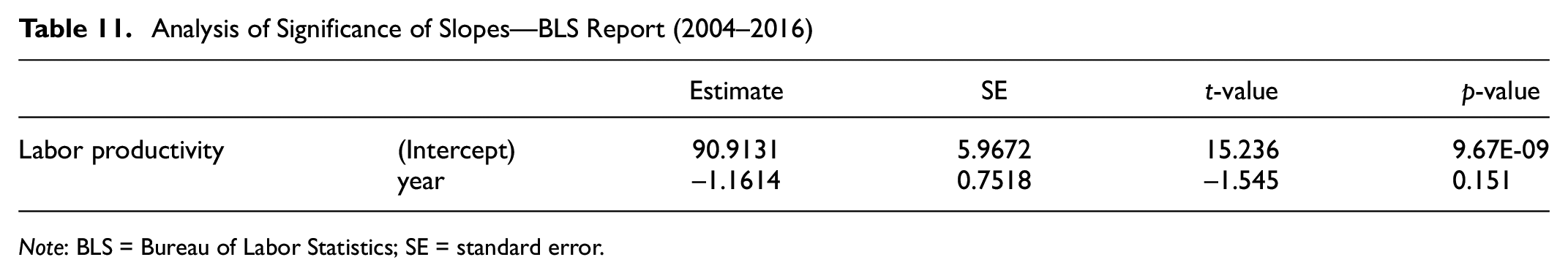
Note: BLS = Bureau of Labor Statistics; SE = standard error.

Figure 6.

Productivity trends—BLS report (2004–2016).

Figure 7.

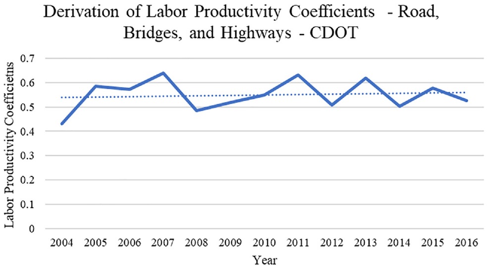
Derivation of labor productivity coefficients—current research (2002–2016).

Furthermore, Figure 7 shows the trend for the overall transportation construction industry using the data analyzed in the current research. Contrary to what is shown in the project-level analyses, the trend of these labor productivity coefficients seems to be increasing (which would mean a decrease in productivity). Nonetheless, the graphical representation does not provide enough information about the trend. Similar to what was computed for new construction, reconstruction, and bridges, additional analysis of the slope provides conclusive information about the trend, showing no significance (Table 12). This information means that the productivity trend is not decreasing.

Table 12.

Analysis of Significance of Slopes—Current Research (2002–2016)

	Estimate	SE	t -value	p -value
(Intercept)	0.536413	0.037743	14.212	2.01E-08
Year	0.001849	0.004755	0.389	0.705

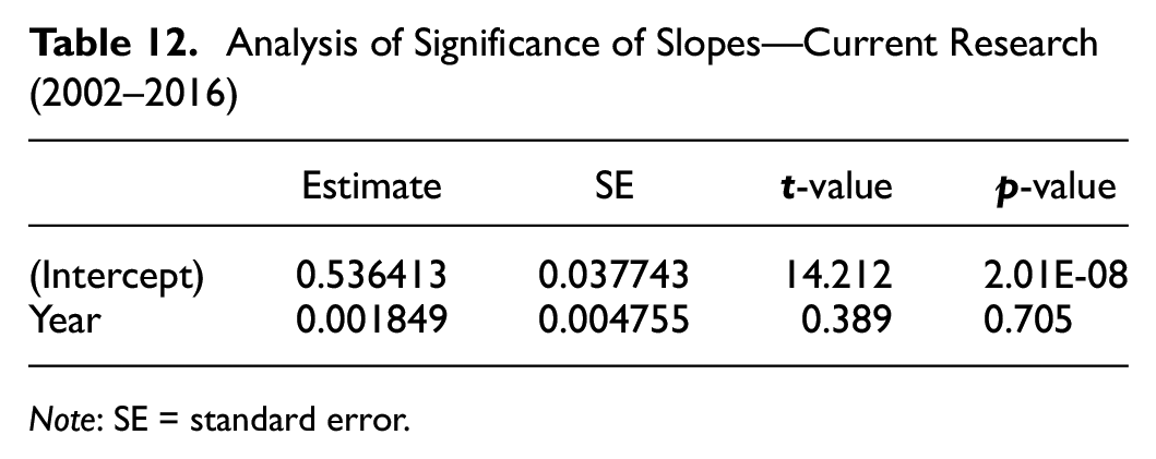
Note: SE = standard error.

When analyzed for the whole transportation construction industry, the data show no significant trends with regard to productivity changes, but when analyzed at the project level, they indicate a significant increase in bridge project productivity, whereas new construction and reconstruction show no significant trends (either an increase or decrease) in productivity (Table 9). The derivation of labor productivity coefficients per project type is shown in Figure 4.

Moreover, the output data presented in the current research provide a higher level of detail than those offered by Sveikauskas et al. ( 2 ), while still producing similar results. In their research, Sveikauskas et al. ( 2 ) used data obtained from the COC that is only collected every five years. In their study, the data had to be interpolated to fill the gaps between surveys. On the other hand, the current research used data obtained from CDOT that had a higher level of detail. The detail is such that it allowed the research team to deflate the cost of construction work installed to a quarterly level using the NHCCI. As pointed out by Sveikauskas et al. ( 2 ), using the NHCCI adds strength to the analysis because, as they say, “The measures are more reliable because the deflators are specifically designed for each industry.”

Finally, the authors of this paper consider that the important contribution it makes is the metric developed, which is easily replicable. This fact should help researchers conduct more extensive studies using data from other state transportation agencies. The metric developed with the current methodology can be used to complement the metrics already developed by other authors. Moreover, the metric developed here could help in understanding where productivity is changing or stagnating at the macro level. This would be useful for the transportation construction industry, because it would then be able to evaluate whether efforts to increase productivity had been effective. Furthermore, the industry would be able to determine where to focus future research efforts, that is, on increasing productivity or on finding the causality of productivity trends.

Footnotes

Author Contributions

The authors confirm contribution to the paper as follows: study conception and design: Guillermo Nevett Fernandez, Paul M. Goodrum; data collection: Guillermo Nevett Fernandez; analysis and interpretation of results: Guillermo Nevett Fernandez, Paul M. Goodrum, Ray L. Littlejohn; draft manuscript preparation: Guillermo Nevett Fernandez, Paul M. Goodrum, Ray L. Littlejohn. All authors reviewed the results and approved the final version of the manuscript

Declaration of Conflicting Interests

The author(s) declared no potential conflicts of interest with respect to the research, authorship, and/or publication of this article.

Funding

The author(s) received no financial support for the research, authorship, and/or publication of this article.

ORCID iD

Guillermo Nevett

References

US Census Bureau. Construction Expenditure. US Department of Commerce. https://www.census.gov/construction/c30/historical_data.html. Accessed September 20, 2018.

Sveikauskas

Rowe

Mildenberger

J. D.

Measuring Productivity Growth in Construction. Monthly Labor Review, Vol. 141, 2018, pp. 1–34.

Teicholz

Labor-Productivity Declines in the Construction Industry: Causes and Remedies (Another Look). AECbytes Viewpoint, Vol. 67, 2013.

Sveikauskas

Rowe

Mildenberger

Price

Young

Productivity Growth in Construction. Journal of Construction Engineering and Management, Vol. 142, No. 10, 2016, Article 04016045.

Sprague

Beyond the Numbers: Below Trend: The U.S. Productivity Slowdown since the Great Recession. U.S. Bureau of Labor Statistics. https://www.bls.gov/opub/btn/volume-6/below-trend-the-us-productivity-slowdown-since-the-great-recession.htm. Accessed November 26, 2019.

Goodrum

P. M.

Haas

C. T.

Glover

R. W.

The Divergence in Aggregate and Activity Estimates of US Construction Productivity. Construction Management & Economics, Vol. 20, No. 5, 2002, pp. 415–423.

Huang

A. L.

Chapman

R. E.

Butry

D. T.

Metrics and Tools for Measuring Construction Productivity: Technical and Empirical Considerations. National Institute of Standards and Technology, Gaithersburg, MD, 2009.

NHCCI. Description – Policy. Federal Highway Administration. https://www.fhwa.dot.gov/policy/otps/nhcci/. Accessed May 17, 2019.

Pieper

P. E.

The Measurement of Construction Prices: Retrospect and Prospect. In Fifty Years of Economic Measurement: The Jubilee of the Conference on Research in Income and Wealth ( Berndt

E. R.

Triplett

J. E.

, eds.), University of Chicago Press, Chicago, IL, 1991, pp. 239–272.

10.

Allen

S. G.

Why Construction Industry Productivity is Declining. National Bureau of Economic Research, Cambridge, MA, 1985.

11.

Allmon

Haas

C. T.

Borcherding

J. D.

Goodrum

P. M.

US Construction Labor Productivity Trends, 1970–1998. Journal of Construction Engineering and Management, Vol. 126, No. 2, 2000, pp. 97–104.

12.

Whiteside

J. D.

Construction Productivity. AACE International Transactions, No. 27, 2006, pp. ES81–88.

13.

Vereen

S. C.

Rasdorf

Hummer

J. E.

Development and Comparative Analysis of Construction Industry Labor Productivity Metrics. Journal of Construction Engineering and Management, Vol. 142, No. 7, 2016, Article 04016020.

14.

Duin

R. P.

Small Sample Size Generalization. Proc., Scandinavian Conference on Image Analysis, Uppsala, Sweden, 1995, pp. 957–964.

15.

Nevett

Goodrum

P. M.

Littlejohn

R. L.

Understanding the Effect of Bid Quantities, Project Characteristics, and Project Locations on the Duration of Road Transportation Construction Projects during Early Stages. Transportation Research Record: Journal of the Transportation Research Board, 2020. 2675: 121–134.

16.

Sheskin

D. J.

Handbook of Parametric and Nonparametric Statistical Procedures. CRC Press, New York, NY, 2003.

17.

Goodrum

P. M.

Zhai

Yasin

M. F.

Relationship between Changes in Material Technology and Construction Productivity. Journal of Construction Engineering and Management, Vol. 135, No. 4, 2009, pp. 278–287.

18.

Thomas

H. R.

Minchin

R. E.

Jr. Chen

Role of Workforce Management in Bridge Superstructure Labor Productivity. Journal of Management in Engineering, Vol. 19, No. 1, 2003, pp. 9–16.

19.

Hancher

D. E.

Taylor

Nighttime Construction Issues. Transportation Research Record: Journal of the Transportation Research Board, 2001. 1761: 107–115.

20.

Teicholz

Goodrum

P. M.

Haas

C. T.

US Construction Labor Productivity Trends, 1970–1998. Journal of Construction Engineering and Management, Vol. 127, No. 5, 2001, pp. 427–429.