
Abstract
Under specific circumstances signal timing at a traffic signal allows the switching of two green times within one cycle. Practitioners expect a reduction in delays and queue length as a result of this control strategy. However, no analytical methodology is available to quantify this effect. To resolve this deficit, analytical considerations have been undertaken. They follow the principles that are also the basis for conventional signal performance analysis. The basic difference compared with a single green is that, within each cycle, the maximum length of the vehicle queue remains shorter under the two-green regime. This effect is expressed by the term uniform delay, w1. For that parameter, a specific deterministic derivation is proposed. The second element is the incremental delay, w2, which stands for the effects of randomness and temporary oversaturation. The analysis confirmed that this parameter could be adopted from conventional methods. Different formulas for the estimation of w2 were investigated using simulation studies. Thus, a set of equations is given for the prediction of average delay and of percentile queue length in the case of two green times. Verification of the derived formulas was performed using Monte Carlo simulations. The results could easily be applied in practice and might be implemented into guidelines. The application demonstrated how a second green within one signal cycle reduced delays and, notably, queue lengths.
Traffic signals, on certain occasions, offer the possibility of two green times to specific signal groups within each cycle time. Here, we discuss two green times that are separated by an intermediate red signal under fixed-time signal control. The potential for two greens is usually reported for pedestrian signals. However, quite frequently this option also exists within signal timing plans for vehicular movements. For right-turn movements particularly, establishing a second green time may be an option in several cases.
In practice, setting a separate second green within one cycle requires the signal controllers to allow this kind of switching, which is usually the case for controllers in central Europe ( 1 ). Also, in the NTCIP (National Transportation Communications for ITS Protocol) and NEMA (National Electrical Manufacturers Association) standards ( 2 , 3 ), a second green time can be implemented using what are referred to as overlaps. In Germany, the cycle time in fixed-time control is usually between 60 and 90 s. In some cases, 120 s is applied. In reality, however, most traffic signals operate in a traffic-responsive manner, differing widely in the level of sophistication used in controlling the traffic. Most of these traffic-actuated signals also follow a sequence based on a fixed-time phasing scheme. Thus, the question of implementing a second green into this type of sequence is also relevant. Controllers allow the switching of signals in every second of the cycle time. In detail, signalization is as follows: it is mandatory that the “green” is announced by “red and yellow” (1 s). Between “green” and the following “red” a “yellow” is displayed for a duration of 3 s (under 50 km/h maximum speed), 4 s (60 km/h), and 5 s (70 km/h). Speed is always limited: the maximum allowed is 70 km/h. The “green” can be displayed as a full green circle, meaning that turning drivers have to give priority to conflicting traffic, that is, opposing traffic and parallel pedestrians and cyclists. The traffic light “green” may also be indicated as an inserted green arrow, which means that conflicting traffic need not be expected (“protected movement”). Inserted green arrows can be applied for right- and left-turning movements as well as for straight ahead traffic. A green arrow signal may be the predominant signalization in the case of two greens for right-turning traffic (“protected right-turn”).
In practice, a second green time is typically implemented into capacity and performance estimation by adding both green times and then treating them as a single green. However, this simple method does not account for the total positive effects that evolve from the second green, which will be demonstrated later in this paper (see Figures 5 and 6).
The purpose of this paper is to present the analytical equations that estimate the average delay and queue lengths in cases of two green times. Here, we concentrated our derivations on cases in which drivers did not have to contend with conflicting traffic during the green (i.e., “protected green”).
Our derivations started from the traditional methodology for estimation of performance measures at traffic signals. These were then expanded to account for the effects of the second green. To validate the resulting equations, simulations were performed. Our conclusions in relation to practical applications are discussed.
Review of Relevant Literature
Documentation was examined in a thorough search of quantitative analyses of the consequences for vehicular traffic generated by double green times during one cycle at a traffic signal. However, no references for scientific research could be identified. In several consulting reports covering real-world cases, their authors expected reductions in delays and queue lengths without being able to quantify their expectations. The application of double greens seemed to be mainly concentrated on right-turn movements in an exclusive lane. However, surprisingly, this solution has also been proposed for protected left-turn movements in a few cases ( 3 , Example 7).
The majority of occasions in which two greens were discussed related to pedestrian signals. In such cases, the determination of delay was not problematic since the maximum delay (which determines the level of service, according to Handbuch fuer die Bemessung von Strassen [HBS; 4 ]) and the average delay (Highway Capacity Manual [HCM; 5 ]) are given by the duration of the red times.
In U.S.-based literature, the problem is covered by the term “signal overlap.” This denotes a green time that is provided within two phases of a signal timing plan. One example is illustrated in Exhibits 5-13 and 5-14 of the Signal Timing Manual ( 2 ). Usually, overlap means a green time that is provided during two succeeding phases. But this kind of phase scheme might also lead to two separate greens within one cycle if the relevant phases are disconnected. A method to estimate the consequences of such a control scheme is not discussed within that manual.
Analytical Solution for Average Delays
The current methodology for the estimation of capacity and traffic performance at traffic signals was based on theoretical analysis. Empirical methods were not the preferred option here since a statistically reliable observation of the required parameters in real traffic did not seem possible.
All the following considerations apply only to a fixed-time signal.
One Movement With One Single Green
As a fundament of all derivations, we start from the estimation of average delay at a traffic signal with one green time per cycle. The classic formula is by Webster, which postulates that the total average delay is the sum of two components ( 6 ),

where w1 = delay caused by the continuous alternation between red and green (referred to as uniform delay in HCM [ 5 ]), s; and w2 = delay caused by randomness in the arrival process and by temporary oversaturation (incremental delay in HCM [ 5 ]), s.
The basic uniform delay, w1, is calculated as (see Webster [ 6 ])

where
U= cycle time,s;
G= effective green time,s;
R= effective red time= U – G,s;
λ= G / U= proportion of green -;
q= traffic volume (demand), vehicles per hour vph;
s= saturation flow = capacity for uninterrupted green, vph
= 3,600 / tb;
tb= departure headway between queued vehicles at the stop line,s;
x= q / C= degree of saturation; and
C= capacity, vph,

This equation is only applicable for x ≤ 1, that is, for undersaturated conditions (q ≤ C). In the case of a time-dependent solution with temporal oversaturation in the considered peak interval (i.e., q > C), this equation is applied with x = 1. Thus, Equation 2 can be written as follows (see HCM Equation 19-19 [ 5 ]):

where
The total consequences of randomness and temporary oversaturation are expressed by the incremental delay term, w2. The incremental delay, w2, is calculated as

where NGE = average length of the queue at the end of green, measured in vehicles veh.
Incremental delay consists of two delay components. One accounts for delay from the effect of random, cycle-by-cycle fluctuations in demand that occasionally exceed capacity. The second accounts for the delay from a sustained oversaturation during the peak interval.
Here, the major problem is the estimation of NGE; several solutions have been published in the past. Here the more relevant equations are specified.
Akcelik ( 7 ):
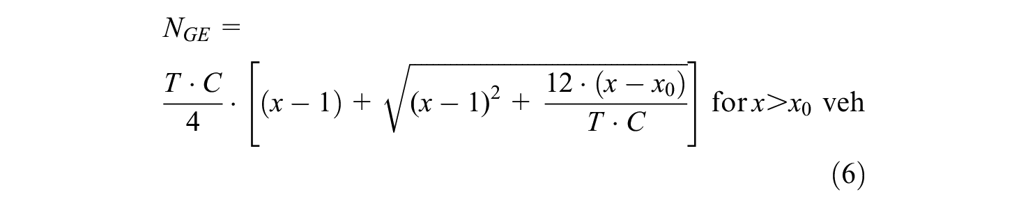
NGE= 0 elsewhere
where
Wu ( 8 ):
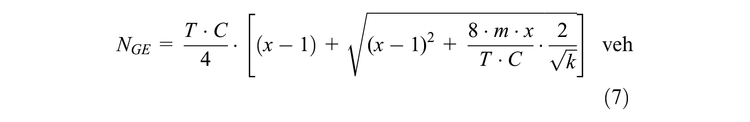
where
M= factor for the degree of randomness in vehicle arrivals;
= 1 for totally random, for example, for an M/M/1 queuing system;
= 0.5 for an M/D/1 queuing system,
=0 for a D/D1 system (= constant headways between arriving vehicles and uninterrupted departures with constant headways).
The best agreement between the simulation (see below) and application of Equation 7 for this study was achieved for m= 0.6.
HCM ( 5 ):
The HCM ( 5 ) indicates the incremental delay, w2, directly via Equations 19 to 26 without referring to NGE, from which it was derived. A transformation of that equation back to NGE for a pretimed signal leads to Equation 8.

HBS ( 4 ):
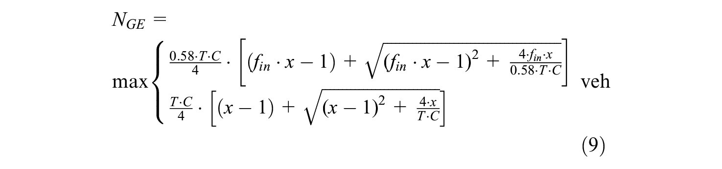
where fin= factor to account for variable traffic flow during the peak hour under concern for T = 1 h –

where q15 = largest traffic volume (demand) during a 15-min interval within the peak hour, vph.
The delay formula (Equation 9) in the HBS ( 4 ) is an extension of the delay formula (Equation 8) from the HCM ( 5 ) to account for the nonstationarity of traffic flow within the peak period of duration, T, by factor fin. If the nonstationarity remains disregarded (i.e., fin = 1), the second line of Equation 9 will always be valid. Thus, in this case the HCM delay formula (Equation 8) and the HBS solution (Equation 9) are identical. Note, the HCM delay formula uses an interval duration of 0.25 h, whereas the HBS delay formula is applied for T = 1 h and, thus, needs adaption to nonstationarity by the term fin to account for variable traffic volumes during the 1-h period.
Unlike the delay formulas in HCM and HBS (Equations 8 and 9), which are based on an M/D/1 queuing system, Equations 6 and 7 consider the specific properties of a queuing system at traffic signals. That is, the departure process is not a steady-state, deterministic one. Instead, the signal creates bunched departures. The maximum number of departures during one green time, expressed by the term k (in Equation 7), accounts for these bunched departures. A queuing system with bunched departures delivers, in general, lower delays compared with an M/D/1 queuing system.
Equation 6 does not consider the queue length, NGE, below a degree of saturation, x0. This leads to an underestimation of delays in this range and a discontinuity of the delay estimation. Also, the simulations described in this paper showed larger discrepancies for Equation 6. Thus, Equation 6 will not be further considered in the following comparisons.
Finally, it must be noted that the whole set of equations (Equations 1 through 9) is only an approximation, since a mathematically exact solution for the delay at signalized intersections under time-dependent conditions is not yet available. All equations for NGE (Equations 6 through 9) account for a peak period of duration T, where the initial queue length is 0 and where the traffic volume after that period is assumed to be 0 as well. The average delay is formed over all vehicles that arrive during the peak period. Thus, the delay that queued vehicles experience after the end of the peak period (until the final queue is completely dissolved) is also attributed to the average. To solve this problem for oversaturated conditions, the coordinate transformation technique (so-called transition technique), which was first established by Kimber and Hollis ( 9 ), is the basis for all the equations mentioned.
One Movement With Two Greens
As a first step, uniform delay, w1, must be determined (see Equation 1). We assume that the cycle starts with a first red R1. The sequence of timing is then: R1→G1→R2→G2. This means the second green ends at the end of the cycle. This convention is only made to illustrate the following derivations. The resulting equations are valid for all kinds of two greens and two reds in one cycle.
To estimate the uniform delay, w1, again, as in the previous section, we have to exclude oversaturation, that is, x ≤ 1.
Here, we use the following terminology:
U= cycle time, s;
G 1= duration of the first green time, s;
G 2= duration of the second green time, s;
R 1= duration of the first red time, s;
R 2= duration of the second red time, s;
“Red time” and “green time” stand for the effective red- and effective green time, s;
a 1= time for the dissipation of the queue from the beginning of the first green time, s;
a 2= time for the dissipation of the queue from the beginning of the second green time, s;
q= traffic volume (≤C), vph;
λ= (G1 + G2) / U= proportion of green;
C= capacity, vph,
s = saturation flow = capacity for uninterrupted green, vph;
= 3,600 / tb;
tb= average departure headway between vehicles at the stop line, s;
x= q / C= degree of saturation.
Here we have to distinguish between three cases (see Figures 1 to 3),
where
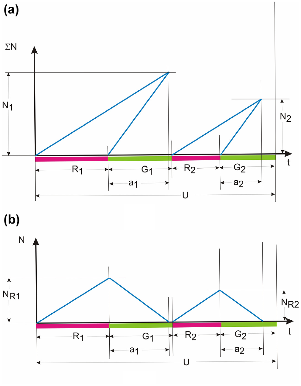
Derivations for Case 1: (a) sum of arriving and departing vehicles and (b) length of the queue.
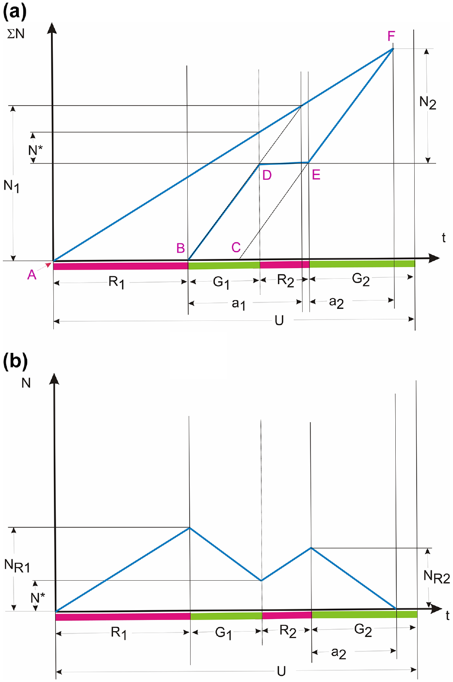
Average queue lengths for Case 2: (a) sum of arriving and departing vehicles and (b) length of the queue.
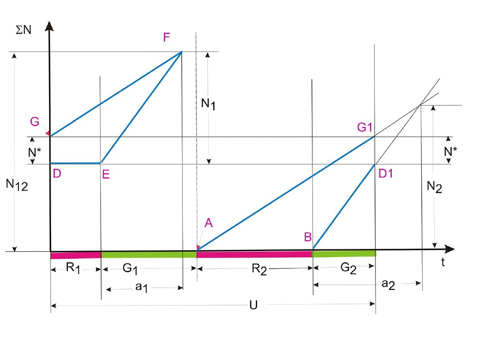
Sum of arrivals (upper blue curve) and departures (lower blue curve) over one cycle for Case 3.
Based on x ≤ 1, more than these three cases is not possible.
We have to remember that the sum of all delays is equal to the area, F, under the curve for the number of queuing vehicles (see Figure 1). Therefore, we have to calculate this area for the three cases. The uniform delay, w1, then is

Case 1:
The maximum number of vehicles in the queue for each of the two subperiods occurs at the end of the relevant red time (Figure 1b). Then the maximum during the whole cycle is

where

The maximum extension of the queue—upstream from the stop line—(back-of-queue [BOQ], Figure 1a) is


The total deterministic delay (sum of all delays) is represented by the area of the two triangles in Figure 1a),

The average deterministic delay is then
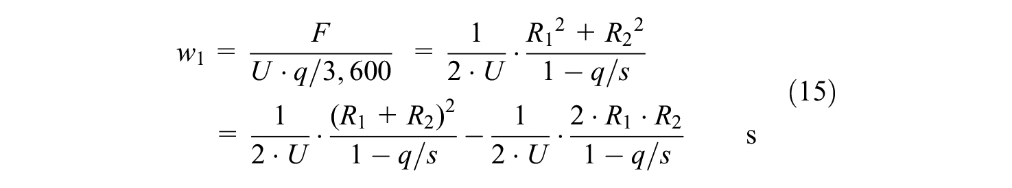
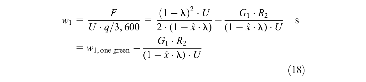
For delay calculation under time-dependent conditions with temporary oversaturation, the degree of saturation can exceed the value of 1 in the peak interval. However, the uniform delay is only calculated below a limit of q / s =

where
w 1,one green
= uniform delay for one green time (G1 + G2) in a cycle (Equation 4) s
Case 2:
F = area within the polygon A – F – E – D – B – A
= area F(A-F-C) - area F(B-D-E-C)

where
The area F represents the sum of all delays. Thus, for
In Figure 2, different parameters for the queue lengths for Case 2 are calculated as follows.
The queue length at the end of the first green is

The maximum number of vehicles at the end of the queue (BOQ) in greens No. 1 or No. 2 is

where


Case 3:
Case 3 is symmetrical to Case 2. Exchanging the indexes 1 and 2 in Case 2 leads to the corresponding equations for Case 3. Thus,

Obviously, if Equations 16, 18, and 21 are compared with Equation 4, two green times in a cycle will always lead to a reduction in delays compared with a single green time (G1 + G2) even if the sum of green times is identical.
Examples and Verification by Simulation
One Single Green
In the first step, the set of equations for the average delay at a traffic signal with only one green per cycle was tested. One purpose of these tests was to identify the best solution for NGE among Equations 6 to 9.
The results from the analytical equations were compared with the simulation results. The Monte Carlo-type simulation generated headways between arriving vehicles either from an exponential distribution or from a hyper-Erlang distribution. The latter could also generate bunched arrivals in the approaching traffic depending on the traffic volume ( 10 ). This represents a traffic stream traveling on a single lane. Figure 4 demonstrates the results for two cases. For both cases: tb = 1.8 s was used, which is equivalent to a saturation flow of s = 2,000 vehicles per second (vps). The curve referred to as “HBS and HCM” was determined by Equations 8 or 9 where fin = 1. The curve called “Wu (1998)” was calculated using Equation 7 where m = 0.6 .
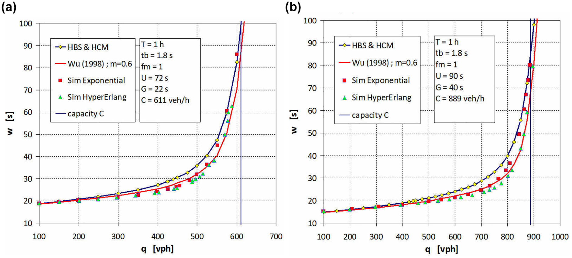
Estimation of average delay depending on traffic volume obtained by four different approaches for two examples: (a) U = cycle time = 72 s; G = green time = 22 s and (b) U = cycle time = 90 s; G = green time = 40 s.
We see here and in other examples that the equations from HBS (or HCM) did not precisely represent the simulation results. In the comparison, only the second line of Equation 9 (for fin = 1) was used, which rendered the results identical to the HCM solution (Equation 19 to 26 in HCM; see Equation 8). Conversely, the solution by Wu ( 8 ), which considered the specific property of bunched departures at a traffic signal, more closely matched the simulated delays, especially for the case of more realistic vehicle arrival patterns (i.e., hyper-Erlang). Also, the fit was not perfect. However, the deviation between the approximate analytical solution and the simulation results in the area for intermediate degrees of saturation was typical for the coordinate transformation technique after Kimber and Hollis ( 9 ).
Compared with the HCM/HBS model (Figure 4), exponential arrivals generated lower delays. This was a result of the imbedded M/D/1 queue in this model, where M means exponentially distributed arrivals. An M/D/1 queue overestimated the delay at signalized intersections where the departure was not steady state (cf. letter “D” for “deterministic” in M/D/1) within the cycle time. Since there was no departure during the red time at all, the departures were not completely deterministic. Deterministic departures only occur during green time. Exponential arrivals provide a better fit at higher flows because this effect becomes less significant at a higher degree of saturation.
As an outcome from these studies the estimation for NGE offered by Equation 7 was regarded as the most realistic solution.
Two Greens in One Cycle
The results from Equations 16, 18, and 21 were tested for the two cases quantified in connection to Figure 5. Here a larger departure headway tb = 2 s (larger than in the previous example) was applied, since this value is typical for right-turn traffic. For both cases in Figure 5 the cycle time is U = 90 s and the sum of green times is 40 s, which means a capacity of 800 vph. The duration of the observed peak period is 1 h. The dependency between traffic volume and delay was analyzed for both cases. The following analytical solutions were applied:
W-HBS (one green): total delay equations according to HBS or HCM (Equations 8 or 9) for the fictitious case of one green (G1+G2),
w (NGE after Wu, m = 0.6): total delay, where delay, w1, is estimated by Equations 16, 18, and 21 for two greens and NGE is estimated by the Wu formula (Equation 7) with m = 0.6 for two green times.
These solutions are compared to simulation results for the total delay, obtained by simulation with hyper-Erlang distributed headways (Sim-HyperErlang in Figure 5).
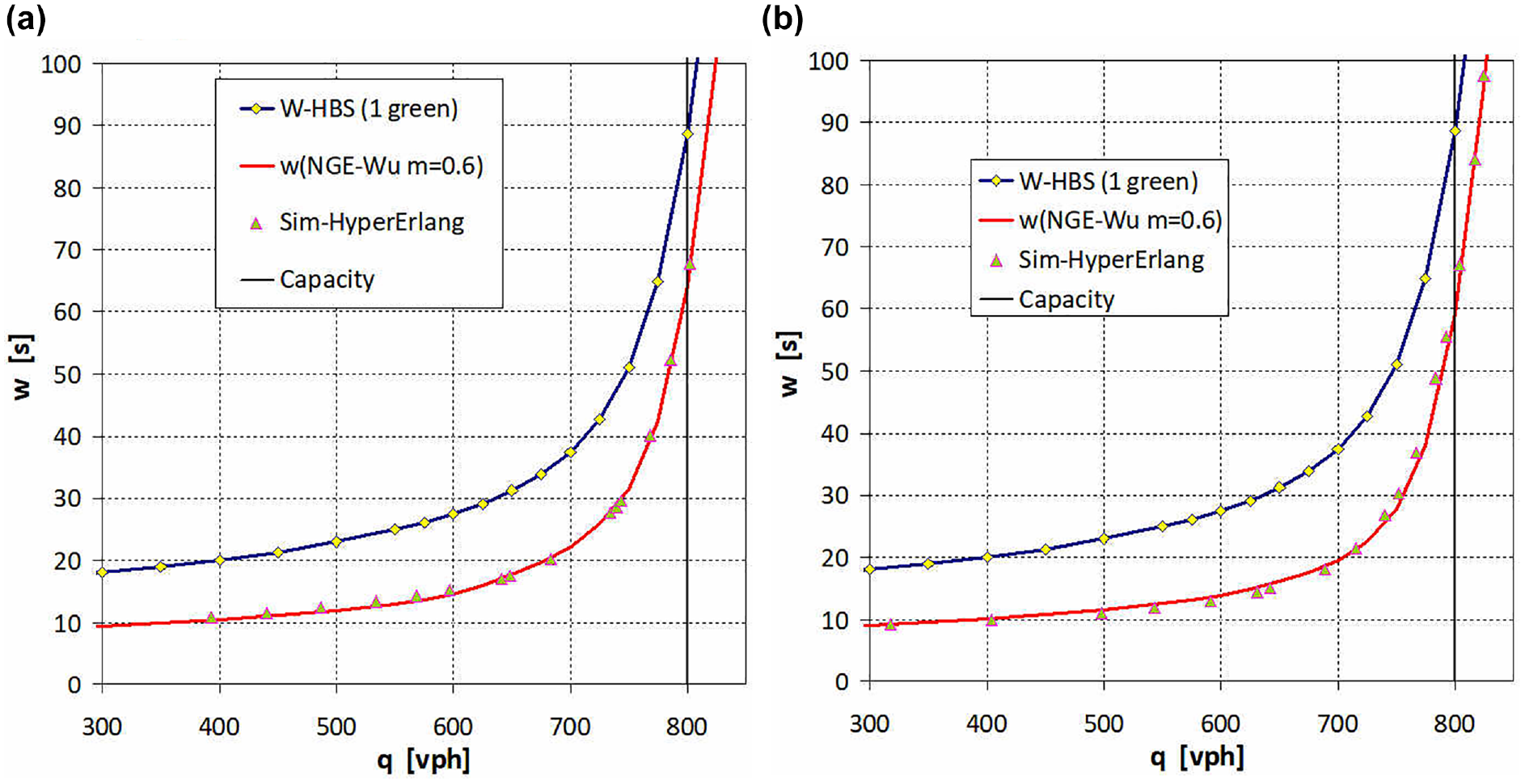
Average delay depending on traffic volume : (a) first green: from sec 10 to sec 40 / second green: from sec 60 to sec 70 and (b) first green: from sec 10 to sec 30 / second green: from sec 55 to sec 75
Figure 5 shows a comparison of the results. It is clear that the approximate use of equations for a single green time of duration G1 + G2 (upper curve) led to an overestimation of delay. The resulting error was rather large—compared with the true value (lower curve)—for low and medium traffic volumes.
Again—also for the case of two greens—the application of Wu’s equation for NGE (Equation 7) with m = 0.6 represented the simulated results very well. The use of this formula led to a nearly perfect fit with the simulated values.
The difference between Figure 5, a and b , is the arrangement of the two green times within the cycle. In Figure 5a, the two greens are different whereas in Figure 5b the two greens are symmetrically arranged within the cycle. The latter led to slightly lower delays, although the difference was quite small.
This result can be treated as confirmation of the following statements:
Application of Equations 16, 18, and 21 within Equation 1 represents the average delay incurred by a traffic stream that is controlled by two green times in each cycle.
Wu’s equation for NGE (Equation 7) is a good representation of the effects of randomness and temporary oversaturation also in case of two greens.
The second green time contributes to a significant reduction in delays.
Queue Lengths and Back-of-Queue
The described derivations can be extended to calculate queue lengths. First, as in the derivation of w1, the lengths of the queue must be obtained for the deterministic case where x ≤ 1. Two kinds of queue length are of interest (cf. Figures 1 and 2):
N R1 or NR2 = number of vehicles in the queue at the end of red time R1 or R2; and
N 1 or N2 = position of the BOQ (given as number of vehicles) in the 1st or 2nd period of the cycle. BOQ we understand to mean the farthest position apart from the stop line where an arriving vehicle is impeded by a preceding vehicle waiting for departure.
These are deterministic values without accounting for the incremental queue at the end of green NGE. Formulas for these terms are given in Table 1.
Equations for Different Kinds of Queue Lengths for the Deterministic Case Where x ≤ 1
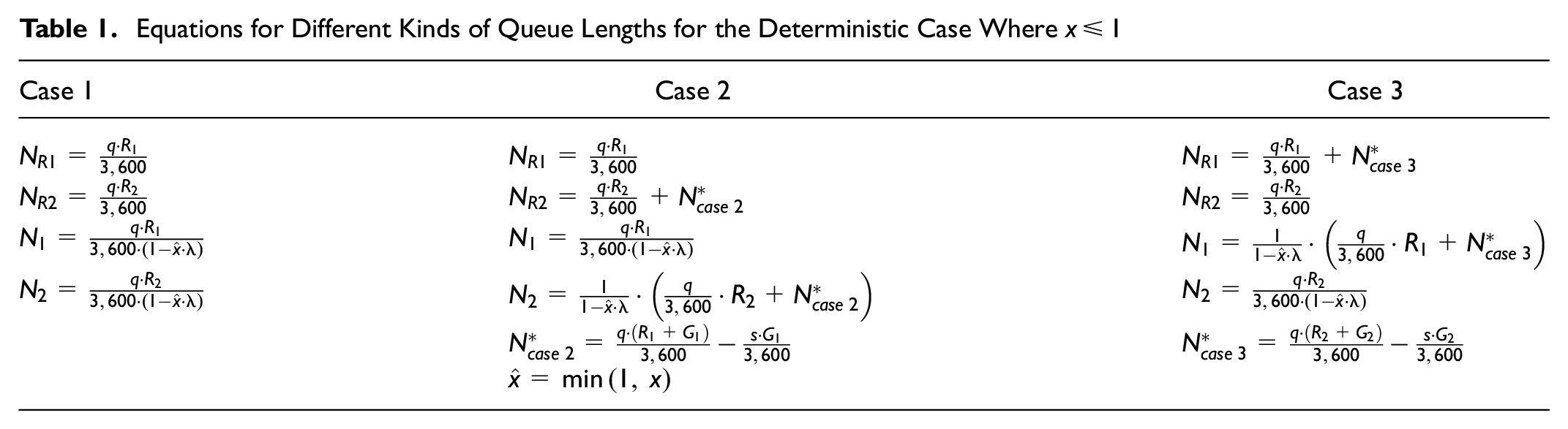
To get the real average queue length,
Within each of the three cases, the maximum number of vehicles in the queue, on average, is

Within each of the three cases the larger BOQ is, on average,

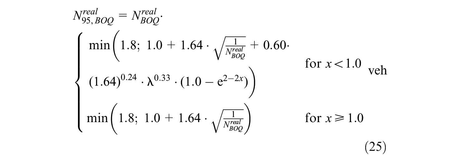
In addition to average queue lengths, practitioners are interested in the maximum expected queue length for the dimensioning of short auxiliary lanes for turning traffic. In many cases the 95th percentile is taken as a representation of the expected maximum. Here the maximum BOQ is of primary interest. To extend the derivations for the average values into percentiles, three approaches have been proposed in guidelines or literature,
• HBS ( 4 ), Figure S4–17 based on the equation

• HCM ( 5 ), Equation 31-150 through 31-153 (the so-called initial queue and the upstream adjustment factor are neglected here for simplification)
• Wu ( 8 )

where
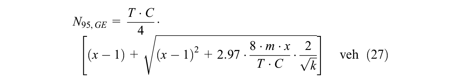

where N1 and N2 have been defined in Table 1; and for m, k refer to Equations 6 and 7.
The three approaches revealed similar results, however, with limited differences.
In Figure 6, the results for the BOQ are illustrated for the same configurations as in Figure 5. The top of the three curves (N95-BOQ one green) represents the 95th percentile of the BOQ for a single green of 40-s duration within a 90-s cycle. This would be the solution for conventional calculations in which the two greens are treated as a single one. The curve in the middle shows the 95th percentile of the BOQ (N95-BOQ two greens) in the case of two greens whereas the lower curve (N-BOQ two greens) indicates the average BOQ (N-BOQ). From the figure we can ascertain that for low and medium traffic volumes the second green time contributes to a quite significant reduction in the maximum queue length. On the other hand, for oversaturated conditions, the second green has, in absolute numbers, a similar effect. However, relatively, the difference becomes less important. It can also be seen, that with balanced green times (Figure 6b, G1 = G2 = 20 s) the queue lengths are smaller than with imbalanced green times (Figure 6a, G1 = 30 s and G2 = 10 s).
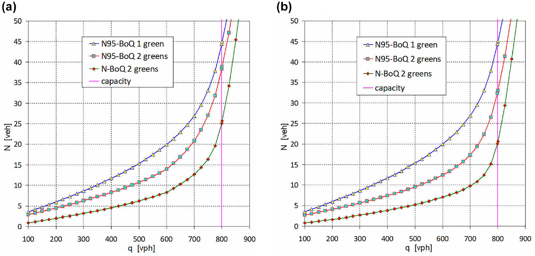
Back-of-queue and its 95th-percentile depending on traffic volume: (a) first green: from sec 10 to sec 40 / second green: from sec 60 to sec 70 and (b) first green: from sec 10 to sec 30 / second green: from sec 55 to sec 75
In interpreting the calculated queue lengths, it should be noted that these values are somewhat artificial as these so-called vertical queues are obtained from queuing theory. Usually, real queue lengths in front of a traffic signal are shorter depending on the speed of vehicles approaching and departing at traffic signals. As a simplified solution, a reduction factor of 0.9 could be applied to the calculated vertical queue lengths to estimate real-world queue lengths (cf. Akcelik [ 7 ] and Wu [ 8 ]).
Conclusion
To date, one shortcoming of traffic signal analysis has been the lack of estimation procedures for traffic performance generated by two green times within one signal cycle. This allocation for signal timing may be mainly applied for right-turn movements. Modern signal controllers should be able to implement corresponding signal switching.
To resolve this deficit in quantitative methods, analytical considerations have been undertaken. They follow the same principles that underlie conventional signal performance analysis. They follow Webster, who postulated that the total average delay can be formed from the sum of uniform delay, w1, and incremental delay, w2 ( 6 ). w1 stands for fluctuation of the queue length during the signal cycle. For this parameter, a specific deterministic derivation was proposed for two greens that included three potential cases for the arrangement of the green times. The second element, w2, stands for the effects of randomness and temporary oversaturation. Here the existing equations for a single green could be adopted. Among the formulas for the estimation of w2 the equation proposed by Wu proved to be the best fit ( 8 ). This formula also has the potential to improve the precision of the delay formulas in the HCM ( 5 ) and HBS ( 4 ). The sequence of Equations 1, 5, and 8 is recommended for estimation of average vehicle delay at a pretimed traffic signal with a single green time.
For the case of two green times within the cycle, a set of equations is given for the prediction of average delay and queue length. Average delay can be estimated by the sequence Equation 1 (Equations 16, 18, or 21), and Equation 8, where the application of Equations 16, 18, or 21 depends on three cases for the arrangement of the two greens within the cycle.
The formulas were validated using Monte Carlo simulations, as were the existing methods. The derivations apply only to fixed-time signal control—like the corresponding methods for single green times. The results are ready to be applied in practice and might be incorporated into guidelines. This application has demonstrated how a second green within one signal cycle could reduce delays and—notably—queue lengths.
Further research should investigate whether and how the results could be extended to applications for actuated signal control. Modification of the results to incorporate permitted movements could also be studied in the future.
Footnotes
Author Contributions
The authors confirm contribution to the paper as follows: study, conception, and design: W. Brilon, N. Wu, R. Koenig; mathematical calculations: W. Brilon, N. Wu, R. Koenig; analysis and interpretation of results: W. Brilon, N. Wu, R. Koenig; draft manuscript preparation: W. Brilon, N. Wu, R. Koenig;. All authors reviewed the results and approved the final version of the manuscript.
Declaration of Conflicting Interests
The authors declared no potential conflicts of interest with respect to the research, authorship, and/or publication of this article.
Funding
The authors received no financial support for the research, authorship, and/or publication of this article.