Telecommuting and Travel during COVID-19: An Exploratory Analysis across Different Population Geographies in the U.S.A.

Abstract

This study explores the impact of the COVID-19 pandemic on telecommuting (working from home) and travel during the first year of the pandemic in the U.S.A. (from March 2020 to March 2021), with a particular focus on examining the variation in impact across different U.S. geographies. We divided 50 U.S. states into several clusters based on their geographic and telecommuting characteristics. Using K-means clustering, we identified four clusters comprising 6 small urban states, 8 large urban states, 18 urban–rural mixed states, and 17 rural states. Combining data from multiple sources, we observed that nearly one-third of the U.S. workforce worked from home during the pandemic, which was six times higher than the pre-pandemic period, and that these fractions varied across the clusters. More people worked from home in urban states compared with rural states. As well as telecommuting, we examined several activity travel trends across these clusters: reduction in the number of activity visits; changes in the number of trips and vehicle-miles traveled; and mode usage. Our analysis showed there was a greater reduction in the number of workplace and nonworkplace visits in urban states compared with rural states. The number of trips in all distance categories decreased except for long-distance trips, which increased during the summer and fall of 2020. The changes in overall mode usage frequency were similar across urban and rural states with a large drop in ride-hailing and transit use. This comprehensive study can provide a better understanding of the regional variation in the impact of the pandemic on telecommuting and travel, which can facilitate informed decision-making.

Keywords

COVID-19 pandemic urban rural telecommuting working from home travel VMT cluster analysis big data

The ongoing health and economic crisis caused by the COVID-19 pandemic and the imposed social distancing measures have led people to adopt telecommuting (working from home or teleworking) arrangements on a large scale. Based on a recent survey, it was found that between February and May 2020, over one-third of the American labor force swapped in-person work with telework, which increased the share of remote working to nearly 50% of the nation’s workforce ( 1 ). These huge changes in work arrangements and people’s subsequent participation in activity travel may have a long-term impact on domestic activity and travel, including how people organize their work, where that work is performed, and how activities and travel are scheduled. Although the impact of the pandemic was evident at some point in virtually all corners of the country, the distribution of the impact varied significantly, both spatially and temporally.

The earliest COVID-19 case in the U.S.A. was reported in Snohomish County, Washington on January 19, 2020 after the infected individual had returned from Wuhan ( 2 ). The virus spread across the country from concurrent initial cases spanning different regions. Notably, the virus initially spread primarily in urban areas and was transmitted through locations where people live, work, and enjoy their leisure time closely with other people ( 3 , 4 ). It subsequently spread to rural areas, thus affecting the entire country in a relatively short period of time. The transmission of the COVID-19 disease and its subsequent impact differed between urban and rural areas ( 5 – 7 ). For example, there was a higher increase in cases (and a higher number of deaths) in urban areas compared with lower cumulative cases in rural areas ( 6 ). The effects on rural populations were severe, with significant negative impacts on unemployment and overall economic conditions ( 8 ). Moreover, rural residents were observed to have lower compliance rates with COVID-related interventions such as mask mandates ( 9 ). The disparity between urban and rural communities suggests there could be significant differences between the populations residing in each in relation to their work arrangements and activity travel behavior during the pandemic. In this respect, the paper aims to examine how the impact of the pandemic on telecommuting and travel varied across different geographies in the U.S.A.

Recent studies have addressed the impact of the pandemic on telecommuting and travel behavior across different counties. For example, based on a primary survey in Australia, Beck and Hensher ( 10 ) found that from late May to early June in 2020, people returned to normal travel, particularly for shopping, social, and recreational activities for which they used private vehicles. Although the use of private vehicles resumed during that period, public transit usage diminished significantly from the start of the pandemic. The authors also suggested that as an immediate response to the pandemic, working from home could be an effective policy measure for reducing travel both during the pandemic and in the post-pandemic world. Astroza et al. ( 11 ) found from a mobility survey in Chile that factors such as higher income, higher education, being female, and a smaller household size increased the propensity to work from home. Individuals who did telework made fewer work and nonwork trips. In general, the highest reduction in number of trips was observed in public transit and ride-hailing usage, whereas the lowest reduction was in number of trips made by walking, in private vehicles, and by motorcycle. Music et al. ( 12 ) found that telecommuting in Canada had increasingly become a dominant working arrangement because of the pandemic and it had greater potential to increase social wellbeing and social sustainability in both urban and rural communities. Several recent studies have examined whether the impact of telecommuting was complementary or substitutive with regard to individual travel demands during the pandemic ( 13 – 16 ). For example, based on county-level data in the U.S.A., Rafiq et al. ( 16 ) found that working from home contributed to a reduction in the number of workplace visits as well as nonworkplace visits that were linked to work trips. These reductions in the number of trips corresponded to a reduction in average person-miles traveled (PMT).

A primary focus of this paper is an examination of the expansion of telecommuting in response to public and private policies to contain the pandemic. The level of telecommuting (working from home) in various cities, regions, and states depended on factors as varied as the proportion of telecommutable jobs to political tradeoffs between the pandemic and its economic impact. The primary research objective was to examine the geographic variations in the impact of the pandemic on travel in general, and on telecommuting in particular. Many of the variations may be caused by intercorrelated factors. Areas with lower population densities have less population interaction; thus, rural areas experienced lower initial levels of the pandemic and there was less impact on travel here. These areas also tend to have a lower proportion of telecommutable jobs and, thus, the ability to respond to any level of spread by working from home is also lower. To address the research question, a process was developed to identify clusters of states with geographic similarities in relation to dimensions associated with the severity of the pandemic. These clusters allow representative areas to be selected to examine the relative impact of the pandemic on travel and the relative efficacy of telecommuting as a response mechanism.

Note that working from home, or teleworking, can be defined as a work arrangement in which workers spend a proportion of their employed hours working from home. Telecommuting is a related term, which can be defined as a sub-set of teleworking but implies explicitly replacing a commute with telecommunications. From this perspective, someone who does not have an office to which to commute is not a telecommuter ( 16 ). In this study, we used the terms teleworking, working from home, and telecommuting interchangeably, because there was limited information in the data utilized to clarify distinctions between these terms.

This exploratory study captured the impact of the pandemic over one full year from March 4, 2020 to March 12, 2021 based on a wide variety of aggregate and disaggregate data sources (i.e., big data). The impact was examined based on a comprehensive descriptive analysis and visual trends of a range of activity travel indicators. In a similar earlier study, we observed the impact of the pandemic on telecommuting and travel with a particular focus on California, but also including three other populous states: New York, Texas, and Florida ( 17 ). The findings of this study are expected to provide valuable insights into the geographic variations in the impact of the pandemic on telecommuting and travel and, thus, provide guidance for future pandemic-related policy initiatives (e.g., response mechanisms, resource allocation).

Data Sources and Study Time Frame

Data were drawn from multiple sources, with some providing aggregate-level information including county and state-level data and others providing disaggregate-level individual- and household-level data. The aggregate-level data included the New York Times COVID-19 data repository ( 18 ), the Maryland Transportation Institute (MTI) COVID-19 Impact Analysis Platform ( 19 ), Google COVID-19 Community Mobility Reports ( 20 ), and data from the Bureau of Transportation Statistics (BTS) ( 21 ). The New York Times dataset contains state- and county-level COVID-19 cumulative cases and deaths since the first domestic case in January 2020. For the MTI dataset, we extracted selected data from the institute’s publicly available web platform that provided a range of U.S. state- and county-level data (e.g., mobility, COVID-19 spread, economy) from January 1, 2020 to the present. The MTI platform contained privacy-protected mobile device location data representing person and vehicle movements (see https://data.covid.umd.edu/). We collected the county-level cross-sectional data for our study time frame (from March 4, 2020 to March 12, 2021). Daily data for the variables that we considered from the MTI were then collapsed into a single day value within the study time window, one value for each county, to generate an average value per day, thus forming the cross-sectional data for that time window. In particular, we considered two variables: percentage of the workforce working from home during the pandemic; and average PMT per day on all modes (car, train, bus, plane, bike, walk, etc.).

The Google COVID-19 Community Mobility Reports provided traveler locations for geographic areas worldwide. The reports categorized activity places by several land-use types, including workplaces, groceries and pharmacies, retail and recreation, parks, transit stations, and residences. The data provided the relative change in numbers of visits to categorized places compared with a pre-pandemic baseline. The baseline represents a typical value for a specified day of the week and is defined as the median value for the five-week period from January 3, 2020 to February 6, 2020. For each land-use category, the baseline represents individual values for each day of the week ( 20 ). Travel data were obtained from the BTS ( 21 ), which provided trips by distance as well as the number of people staying at home at aggregate state and county levels from January 2019 to June 2021. These trips included travel by all modes. Travel statistics were estimated based on the anonymized national panel of mobile device data. Trips were defined as movements that resulted in a stay longer than 10 min at an anonymized location away from home ( 21 ). We used traffic volume trends data ( 22 ) to analyze the changes in vehicle-miles traveled (VMT) in each of the months of 2020 compared with the same month in the previous year.

The disaggregate-level data utilized included the Household Pulse Survey 2020 to 2021 ( 23 ) and the COVID Future Wave 1 Survey ( 24 ). The Census Pulse Survey includes data on travel behavior collected during phase 2 (August 13–October 26, 2020) and phase 3 (October 28–March 29, 2021) of the survey over two-week periods. These data contain the total number of households substituting in-person work for telework in a given state. More specifically, the survey dataset contains users’ binary response to the following question: “whether an adult in the household substituted some or all of their typical in-person work for telework because of the coronavirus?” The Future Wave 1 Survey provided individual- and household-level data including employment, shopping, travel, attitudes, and demographics. This dataset was gathered from April 14 to October 14, 2020 for a total of 8,723 respondents from across the U.S.A.

For the study time frame, we divided one full year of the pandemic from March 4, 2020 to March 12, 2021 into four time windows based on both conventional seasons and the degree of infection in the U.S.A. These four windows were the spring 2020 outbreak period, summer, the fall increase period, and the 2021 vaccine period. The spread of the pandemic in the U.S.A. over the one-year period and the study time windows are depicted in Figure 1. There was a slightly higher spread in the summer than during the initial outbreak period. During the fall the number of infections increased significantly followed by a sharp decline starting in 2021, at least in part because of vaccination efforts.

Figure 1.

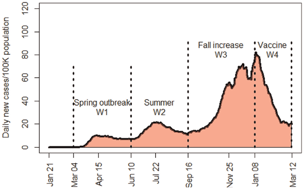
Daily new COVID-19 cases and selected time windows for the U.S.A.

The objective of this study was to explore how the adoption of telecommuting, and activity travel behavior in the U.S.A. varied spatially and temporally during the COVID-19 pandemic. The spatial variations were primarily examined at the state level although in some cases county-level analyses were also conducted based on the availability of data. At the county level, classification as urban or rural was made using data from the 2013 urban–rural classification framework produced by the National Center for Health Statistics (NCHS). According to this framework, all the U.S. counties (3,142) were classified as urban or rural based on the U.S. Census Bureau geographic definitions (classification details can be found in Ingram and Franco ( 25 ).

To explore the spatial variation of the impact of the pandemic systematically, we developed a strategy to identify clusters of states with similar geographic characteristics based on four attributes: fraction of urban counties; fraction of population in urban counties; fraction of area occupied by urban counties; and fraction of workforce who worked from home during the study window. We then selected representative states from each of the clusters identified to examine detailed changes in telecommuting and travel behavior over the study periods. The methodology used to identify clusters and the subsequent analyses are described in the next section.

Methodology

Selection of Study Geographies

We divided the 50 U.S. states clusters based on their geographic characteristics and the degree to which they adopted working from home during the pandemic. We postulate that despite variations, states can be grouped into a small number of heterogeneous clusters in which states in the same cluster would demonstrate similar geographic and work-from-home characteristics, whereas the states belonging to different clusters would show different geographic and work-from-home characteristics. To this end, we computed a set of numeric quantities for each state as a feature vector and utilized a K-means clustering algorithm on that feature space to classify state clusters. We consider the following four quantities (each are real numbers between 0.0 to 1.0) as a feature vector for a given state:

a) fraction of urban counties (using NCHS) in that state;

b) proportion of population living in these urban counties;

c) proportion of land area occupied by these urban counties;

d) fraction of workforce working from home in that state.

Let X_i denote the feature vector for state i, where X_i[l] is the l-th feature value (l = 1, 2, 3, and 4). We define the difference between two states i and j as the Euclidean distance between the corresponding feature vectors X_i and X_j, that is:

‖ X_{i} - X_{j} ‖ = \sqrt{\sum_{l = 1}^{4} {(X_{i} [l] - X_{j} [l])}^{2}}

(1)

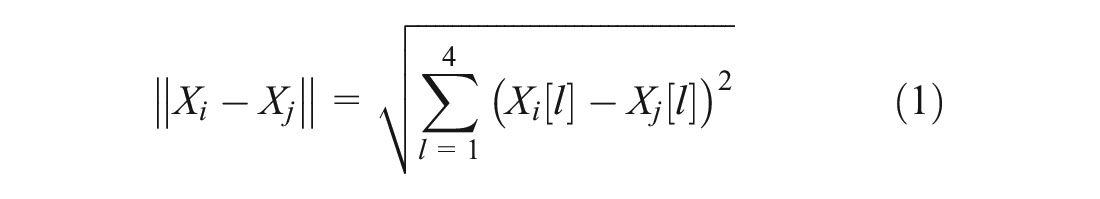
Based on this distance function, the K-means clustering algorithm identifies K clusters among the 50 U.S. states. The clustering algorithm attempts to partition the data into K disjoint clusters, each denoted as C_k (k = 1, 2, …K), where each cluster C_k contains one or more U.S. states and each state is assigned to exactly one cluster. The goal of clustering is to determine clusters so that the sum of pairwise differences among states within the same cluster is minimized, that is:

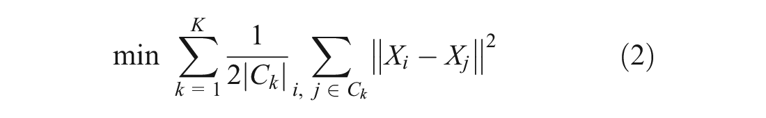
\min \sum_{k = 1}^{K} \frac{1}{2 | C_{k} |} \sum_{i, j \in C_{k}} ‖ X_{i} - X_{j} ‖^{2}

(2)

In the above, $| C_{k} |$ denotes the size of the k-th cluster. For each cluster k, a mean vector, $μ_{k}$ , can be computed by taking an average of members in that cluster, as follows:

μ_{k} [l] = \frac{1}{| C_{k} |} \sum_{i \in C_{k}} X_{i} [l], l = 1, 2, 3, and 4

(3)

With the above, equation (1) can be rewritten as follows:

\min \sum_{k = 1}^{K} \sum_{i \in C_{k}} ‖ X_{i} - μ_{k} ‖^{2}

(4)

An iterative algorithm ( 26 ) was used to find clusters C_k with the above objective as follows:

a) Initialize: assign, randomly, each state to some C_k, for k = 1, 2, …, K.

b) Compute mean vector $μ_{k}$ of each cluster on the current cluster C_k assignment according to equation (3).

c) Reassign cluster C_k based on new $μ_{k}$ ’s, assign state i to the nearest cluster. That is, assign state i to C_k if $X_{i} - μ_{k}$ is the smallest among all clusters. That is, reconstruct each cluster C_k as follows:

C_{k} = {i | ‖ X_{i} - μ_{k} ‖ \leq ‖ X_{i} - μ_{k'} ‖, for k' \neq k}

d) Repeat steps (b) and (c) until convergence (assignments do not change anymore).

The algorithm takes K, the total number of clusters to be determined, as a sole parameter that needs to be specified by the user. Typically, a range of potential values for K (e.g., from 2 to 10) is specified, and the results are evaluated based on the following: (a) whether the fitness of clustering is deemed good, measured by some well-known metric such as within sum of squares (WSS) or silhouette score ( 26 ); and (b) the degree of interpretability of the clusters according to their constituent members. Based on this, one K is chosen as the best.

Exploring Telecommuting and Travel across Selected Geographies

Ideally, telecommuting and travel characteristics of all 50 states during the first year of the pandemic would be shown in this paper. However, displaying 50 states with all the activity travel indicators will be cumbersome. In addition, this will not show any discernable activity travel characteristics across states during the pandemic. Instead, we first clustered the 50 U.S. states into groups based on their geographic characteristics and level of adoption of telecommuting and then selected three representative states from each of the clusters identified. Our hypothesis was that states having similar geographic features and level of adoption of telecommuting would experience similar changes in activity travel characteristics during the pandemic. Thus, this systematic way of clustering all states and selecting “representative” states from each cluster enabled the spatial variations in the impact of the pandemic on telecommuting and travel across clusters to be observed, and led to general conclusions with regard to both similarities and differences according to geographic attributes.

The changes in telecommuting behavior during the pandemic were examined according to the proportion of time spent working from home, changes in the number of workplace visits, the substitution of in-person work for telework, and trends in teleworking. Similarly, the changes in activity travel behavior were explored based on several activity travel analytics, including activity participation by land use, trips by distance, PMT, VMT, and mode usage during the pandemic. The next section describes our results from the cluster analysis and findings with regard to the impact of the pandemic on telecommuting and travel for each identified cluster. In addition to the state-level analysis, some county-level analyses are also discussed.

Results and Discussion

This section presents the results from the cluster analysis and the changes in telecommuting and travel behavior across the identified clusters over the study time periods.

Four Geographies

We conducted K-means clustering on 50 U.S. states for a cluster range of 2 to 12. The results of the goodness of fit with regard to WSS (total WSS) are shown in Figure 2a. The WSS score measures the sum of the square of the distance from each data point to the cluster center, as per equation (4). Ideally, the lower the WSS score, the better the clustering. Usually, WSS scores are higher at smaller values of K (fewer clusters) and progressively decrease as K increases. In a plot of WSS against K, a point in the plot, the “elbow point” defines where the decrement of WSS with respect to K transitions from a relatively sharp decline to a flattening of WSS (also known as a scree slope). We see that an “elbow point,” which represents statistical stability, corresponds to K = 4 in Figure 2a. We utilize these four clusters for subsequent analyses.

Figure 2.

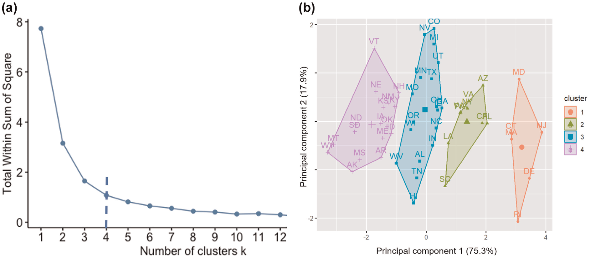
(a) Goodness of fit, (b) K = 4 cluster plot.

The four clusters of 50 states are formed based on four feature attributes that give rise to a four-dimensional representation of data points, which is hard to visualize in a 2-D space. For visual illustration, we resort to the classical principal component analysis, which for a given number of data points finds several orthogonal directions (also known as axes or principal components) for which the data points demonstrate the largest variations. Figure 2b shows such a 2-D representation of 50 states in which the two axes are defined by two principal components that explain the greatest proportion of the variation in the feature space across states. The first component (on x-axis) describes the largest variation (75.3% of the total variance) and the second component (on y-axis) describes the second largest variation (17.9% of the total variance). The states that belong to the same cluster were given the same color, forming a colored region for each of the four clusters. The nonoverlapping cluster regions suggested that the constructed clusters were well defined.

Table 1 provides the means for the feature values of states that belong to a given cluster. Cluster 1 primarily consists of urban counties (91%) and the proportion of the state population living in urban counties is very high (98%). Cluster 1, which has the smallest mean land area and the highest population density, is labeled as “small urban states.” The second cluster also has a higher urban fraction but its land area is much higher than cluster 1. This group is deemed “large urban states.” The third cluster has a mix of urban and rural states (0.33% of land is urban whereas about 80% of the population live in urban counties). The fourth cluster, with the highest average land area and a smaller population density, consists of states with predominantly rural counties (only 20% of counties are urban in this cluster). Thus, this cluster is identified as “rural states.” Note that the fraction of the workforce working from home is higher in urban states compared with rural states.

Table 1.

Mean Characteristics of the Four Clusters Identified

Cluster	Proportion of urban counties	Proportion of population living in urban counties	Proportion of land area occupied by urban counties	Fraction of those working from home in the study window	Average land area (square miles)	State population density (persons per square mile)	Political orientation (% of blue states)
1	0.91	0.98	0.91	0.36	5,449	815.19	100.0
2	0.58	0.90	0.58	0.34	66,025	215.22	66.7
3	0.38	0.80	0.33	0.33	70,769	126.66	50.0
4	0.20	0.55	0.17	0.29	95,611	43.04	29.4

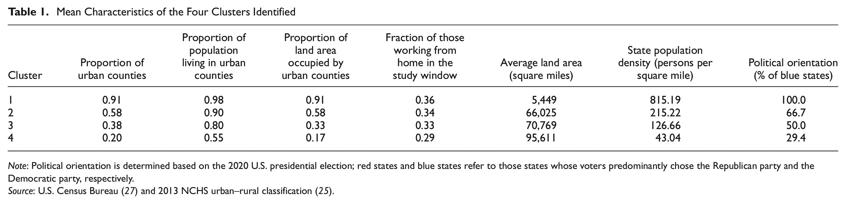
Note: Political orientation is determined based on the 2020 U.S. presidential election; red states and blue states refer to those states whose voters predominantly chose the Republican party and the Democratic party, respectively.

Source: U.S. Census Bureau ( 27 ) and 2013 NCHS urban–rural classification ( 25 ).

The clustering produced splits of 6, 9, 18, and 17 states in the respective clusters (the complete list is provided in Table 2). The map shown in Figure 3 depicts the geographic distribution of the four clusters, with urban states mostly in eastern and western coastal areas, whereas rural and mixed states are in the central area. We chose three representative states from each cluster to analyze trends observed throughout the study window. The selected states for each cluster are marked in bold and underlined.

Table 2.

The Four Clusters Identified and List of States per Cluster

Cluster	Cluster label	Number of states	States
1	Small urban states	6	Connecticut (CT), Delaware (DE), Maryland (MD), Massachusetts (MA), New Jersey (NJ), Rhode Island (RI)
2	Large urban states	9	Arizona (AZ), California (CA) , Florida (FL) , Louisiana (LA), New York (NY), Pennsylvania (PA) , South Carolina (SC) Virginia (VA), Washington (WA)
3	Urban–rural mixed states	18	Alabama (AL), Colorado (CO), Georgia (GA), Hawaii (HA), Illinois (IL), Indiana (IN), Michigan (MI) , Minnesota (MN), Missouri (MO), Nevada (NV), North Carolina (NC), Ohio (OH), Oregon (OR) , Tennessee (TN), Texas (TX) , Utah (UT), West Virginia (WV), Wisconsin (WI)
4	Rural states	17	Alaska (AK), Arkansas (AR), Idaho (ID), Iowa (IO), Kansas (KS), Kentucky (KN), Maine (ME), Mississippi (MS), Montana (MT), Nebraska (NB), New Hampshire (NH), New Mexico (NM) , North Dakota (ND) , Oklahoma (OK), South Dakota (SD), Vermont (VT), Wyoming (WY)

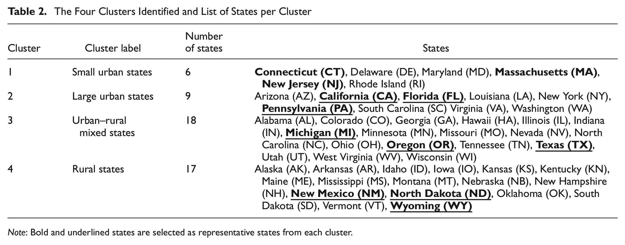
Note: Bold and underlined states are selected as representative states from each cluster.

Figure 3.

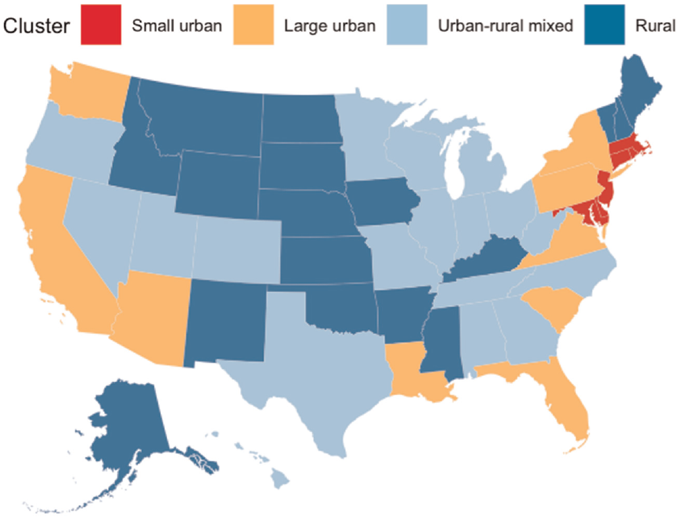
Distribution of U.S. states for the four cluster results.

Pandemic Spread in Four Geographies

Figure 4 displays the differences in the intensity and spread of the COVID-19 infection rates over the one-year study period for our representative states from each cluster. For example, small urban states experienced pandemic waves in the early phase of the pandemic (the spring 2020 outbreak), whereas infections in large urban states started increasing in summer 2020 and reached a peak in fall 2020. Compared with the other clusters, cluster 3 states (urban–rural mixed states) experienced lower peaks of daily infection cases during fall 2020. On the other hand, states belonging to cluster 4 (rural states) experienced pandemic waves relatively later in the year: a single pandemic wave with the highest peak was observed for rural states in the fall 2020 period.

Figure 4.

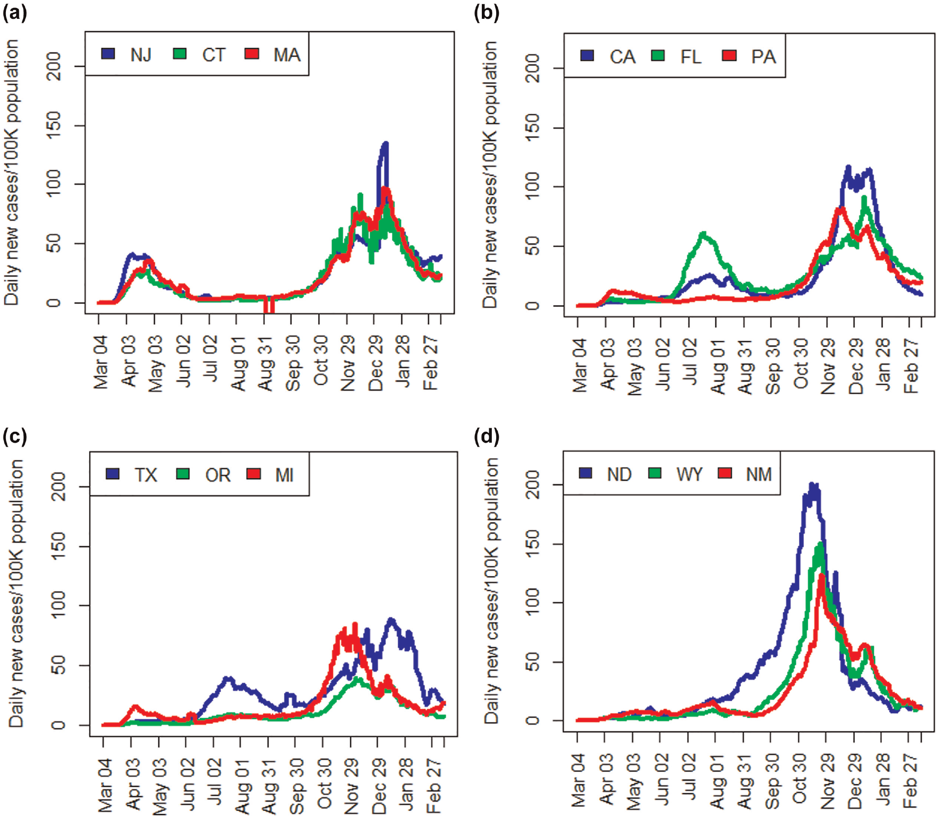
Daily new COVID-19 cases per 100,000 population from January 2020 to March 2021: (a) small urban states, (b) large urban states, (c) urban–rural mixed states, and (d) rural states.

Adoption of Telecommuting during the Pandemic

The changes in telecommuting behavior during the pandemic through March 2020 are discussed from four perspectives: (a) changes in the proportion of people working from home; (b) changes in the number of workplace visits; (c) substitution of in-person work for telework; and (c) trends in teleworking.

Changes in Working from Home and Number of Workplace Visits

Table 3 reports the percentage of the workforce working from home pre-pandemic and during the pandemic in the U.S.A. in the four identified state clusters and for the three selected representative states in each cluster. Although the fraction of people working from home pre-pandemic was 4.7% in the U.S.A., that fraction became 32.2% during the first year of the pandemic, about six times higher than the pre-pandemic level. The table also shows the same fraction for the four defined study periods. The second (summer) period was observed to have the largest percentage of people working from home, whereas the fourth (vaccine) period had the smallest share. On average, more people in urban states worked from home compared with rural states (work-from-home fractions across rural states remained at or below 30%, whereas for urban states they were 30% and above). Brooks et al. ( 28 ) report a similar finding of there being a higher fraction of people working from home in urban states compared with rural states. Among urban states, the largest share of working from home was in small urban states, followed by large urban and mixed state clusters.

Table 3.

Percentage of People Working from Home Pre-pandemic and during the Pandemic

		Analysis windows
	Pre-COVID-19	Spring outbreak period	Summer period	Fall increase period	Vaccine period	During COVID-19
	Jan 3–Feb 6, 2020	Mar 4–June 10	June 10–Sept 16	Sept 16–Jan 8	Jan 8–Mar 12	Mar 4, 2020–Mar 12, 2021
U.S.A.	4.7	28.6	37.3	33.9	27.1	32.2
Small urban states	4.7	34.6	41.3	38.7	32.0	37.1
New Jersey	4.4	35.6	42.8	39.8	33.7	38.4
Connecticut	5.1	35.4	41.0	37.1	29.6	36.4
Massachusetts	5.0	32.5	39.1	37.9	30.8	35.6
Large urban states	5.4	30.6	39.3	36.7	30.4	34.7
California	5.7	30.9	39.6	36.7	29.1	34.6
Florida	5.9	30.1	39.9	37.1	31.7	35.1
Pennsylvania	4.6	30.8	38.3	36.4	30.1	34.4
Urban–rural mixed states	4.7	31.5	40.4	36.6	30.3	35.1
Texas	4.6	31.7	40.2	35.9	29.5	34.8
Oregon	6.8	26.3	36.0	32.5	24.8	30.5
Michigan	3.9	33.1	43.0	40.3	35.2	38.2
Rural states	5.0	25.6	35.3	32.1	25.1	30.0
North Dakota	4.9	23.8	34.2	30.7	24.0	28.6
Wyoming	5.2	21.9	31.3	27.8	19.7	25.8
New Mexico	4.8	27.9	36.1	33.3	25.6	31.3

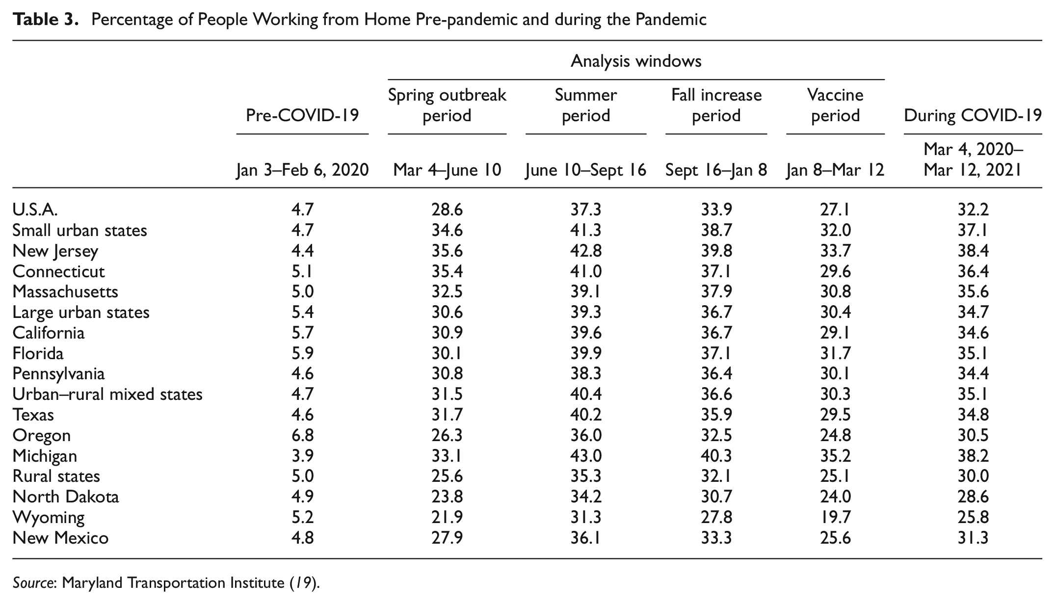
Source: Maryland Transportation Institute ( 19 ).

A higher percentage of people working from home corresponded to a greater reduction in the number of workplace visits during the pandemic. Table 4 shows the changes in the number of workplace visits compared with the baseline (January 3–February 6, 2020) in 4 clusters and 12 selected states. Because the number of workplace visits fell during the pandemic, the changes with respect to the baseline are negative. As expected, the reduction in the number of workplace visits was about the same degree as the percentage of people working from home in all states. Overall, there was a higher reduction in the number of workplace visits in urban states compared with rural states. The largest reduction was in small urban states, followed by large urban states and urban–rural mixed states.

Table 4.

Changes in Number of Workplace Visits (%) during the Pandemic Compared with the Baseline

	Analysis windows
	Spring outbreak period	Summer period	Fall increase period	Vaccine period	During COVID-19
	Mar 4–June 10	June 10–Sept 16	Sept 16–Jan 8	Jan 8–Mar 12	Mar 4, 2020–Mar 12, 2021
U.S.A.	−27.6	−24.7	−22.5	−20.5	−24.1
Small urban states	−39.1	−31.0	−29.3	−30.1	−32.5
New Jersey	−40.6	−31.8	−30.7	−31.5	−33.7
Connecticut	−35.5	−29.8	−26.0	−25.2	−29.4
Massachusetts	−39.1	−30.5	−29.2	−31.0	−32.5
Large urban states	−30.4	−27.7	−25.8	−23.0	−27.1
California	−32.9	−30.2	−29.2	−28.3	−30.3
Florida	−27.5	−27.6	−24.3	−19.7	−25.2
Pennsylvania	−31.3	−25.5	−24.4	−21.8	−26.1
Urban–rural mixed states	−28.1	−25.3	−22.9	−22.1	−24.8
Texas	−25.3	−26.8	−23.5	−23.8	−24.8
Oregon	−29.2	−26.3	−25.3	−24.1	−26.4
Michigan	−34.1	−21.4	−20.6	−17.6	−24.1
Rural states	−28.2	−25.5	−26.1	−23.2	−26.1
North Dakota	−24.0	−22.4	−22.4	−16.6	−21.9
Wyoming	−24.7	−20.9	−19.7	−15.0	−20.7
New Mexico	−29.8	−27.8	−30.6	−28.6	−29.4

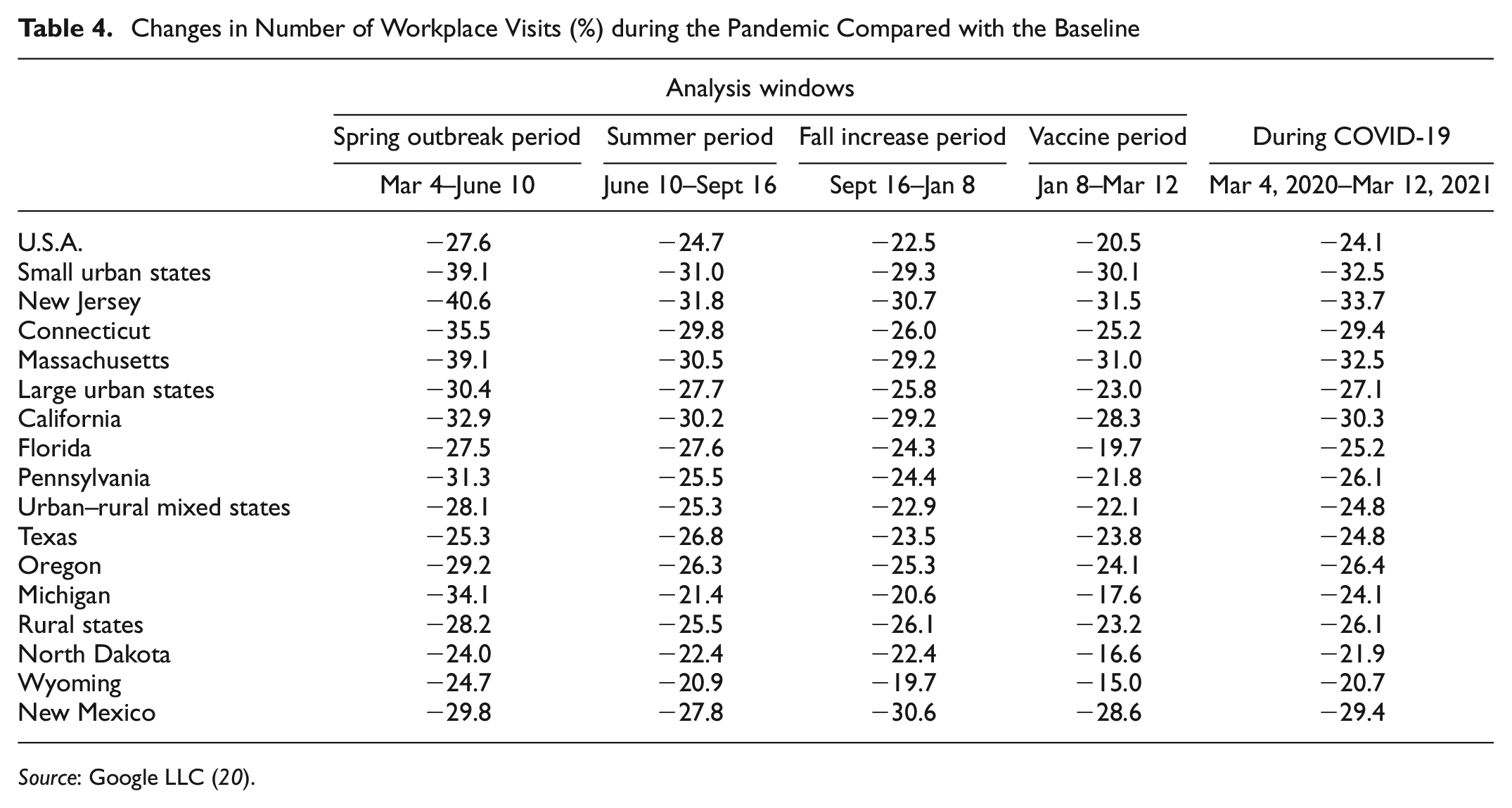
Source: Google LLC ( 20 ).

Substitution of In-Person Work for Telework

Because a considerable fraction of people substituted their in-person work for telework during the pandemic, we observed a greater reduction in the number of workplace visits and at the same time a greater adoption of working from home. Now we want to see what fraction of households in the U.S.A. were actually able to work from home. Figure 5 shows the percentage of households in which at least one adult member from the household substituted in-person work for telework in the sample U.S. states with reference to the whole U.S.A. Note that, here, data are shown from August 2020 to March 2021 because the corresponding survey data were collected starting in August 2020. Nearly 35% of U.S. households adopted the phenomenon of working from home, which meant about one-third of the workforce were doing so during the pandemic. In general, there was a higher rate of substitution in urban states compared with rural states (the substitution rates in small urban states and in rural states were above and below the U.S. national average, respectively).

Figure 5.

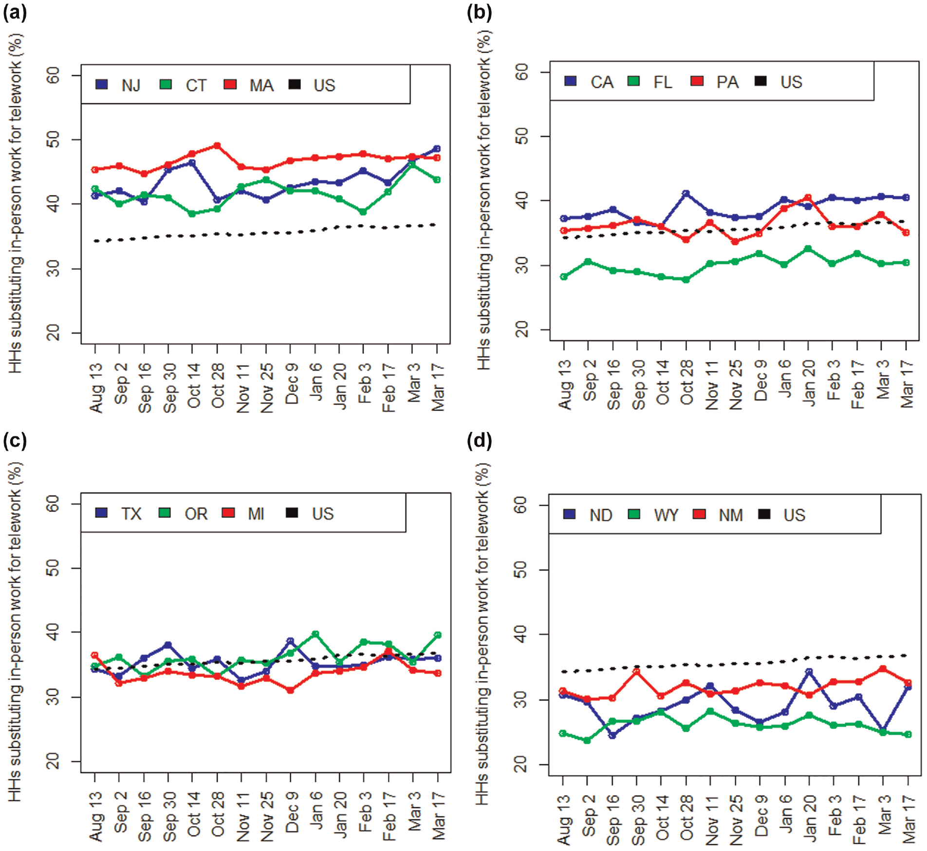
Households with at least one adult substituting in-person work for telework from August 2020 to March 2021: (a) small urban states, (b) large urban states, (c) urban–rural mixed states, and (d) rural states.

Trends in Teleworking

Next, we examined the trends in working from home before, during, and after the pandemic. To examine these changes, we used individual-level data from the COVID Future Wave1 Survey ( 24 ), which was conducted from April 14 to October 14, 2020. There were 8,723 survey respondents across the U.S.A. We examined the trends of working from home in our four identified clusters and the variations in trends across the cluster states as illustrated in Figure 6.

Figure 6.

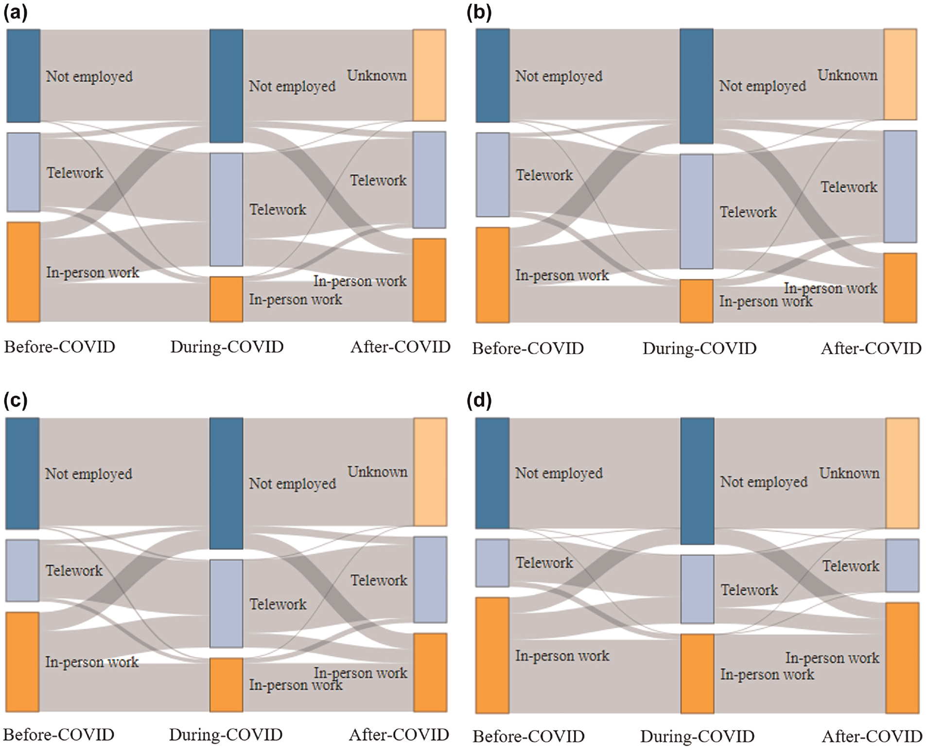
Trends in teleworking before, during, and after the pandemic: (a) small urban states, (b) large urban states, (c) urban–rural mixed states, and (d) rural states.

The general trend was that a greater fraction of the workforce worked from home during the pandemic compared with the pre-pandemic period. If we compare the four cluster states, in rural states, a higher fraction of the workforce were unemployed and a smaller fraction of workers worked from home before and during the pandemic compared with urban states. This implies that during the pandemic, a greater fraction of workers were able to substitute their in-person work for telework in urban states compared with rural states.

With regard to the prospects for telecommuting, a higher fraction of workers who worked from home during the pandemic (in both rural and urban states) reported their preference for continuing to do so even after the threat from the pandemic had lessened. These findings were consistent with other recent surveys in which employers and employees were asked whether they were amenable to continue telecommuting in the post-pandemic world. For example, the Society for Human Resource Management surveyed U.S. employees about their work preferences after the threat from the pandemic had abated and found that 31% of workers preferred to work fully remotely, whereas 31% preferred fully in-person ( 29 ).

Activity Travel Behavior during the Pandemic

This section describes the changes in activity travel behavior across the four clusters during the first year of the pandemic. Among many typical measures of travel behavior, in this study we considered five commonly understood travel dimensions: activity participation by purpose; trips by distance; PMT; VMT; and mode usage.

Changes in Activity Participation by Land Use

Figure 7 shows the percentage changes in number of activity visits or visitors for four land-use (activity) types: workplace, grocery and pharmacy, retail and recreation, and parks, over a one-year period (March 4, 2020–March 12, 2021) with respect to a pre-pandemic baseline value. The baseline for a given type of activity is a typical weekday (calculated over seven days) measured as the median value for five weeks of data between January 3 and February 6, 2020. The baseline and visitor data are defined for U.S. counties, which are then aggregated to generate the state-level data. The mobility data (obtained from Google’s Community Mobility Reports) provide the daily changes in the number of visits by defined land-use (activity) types throughout the pandemic periods.

Figure 7.

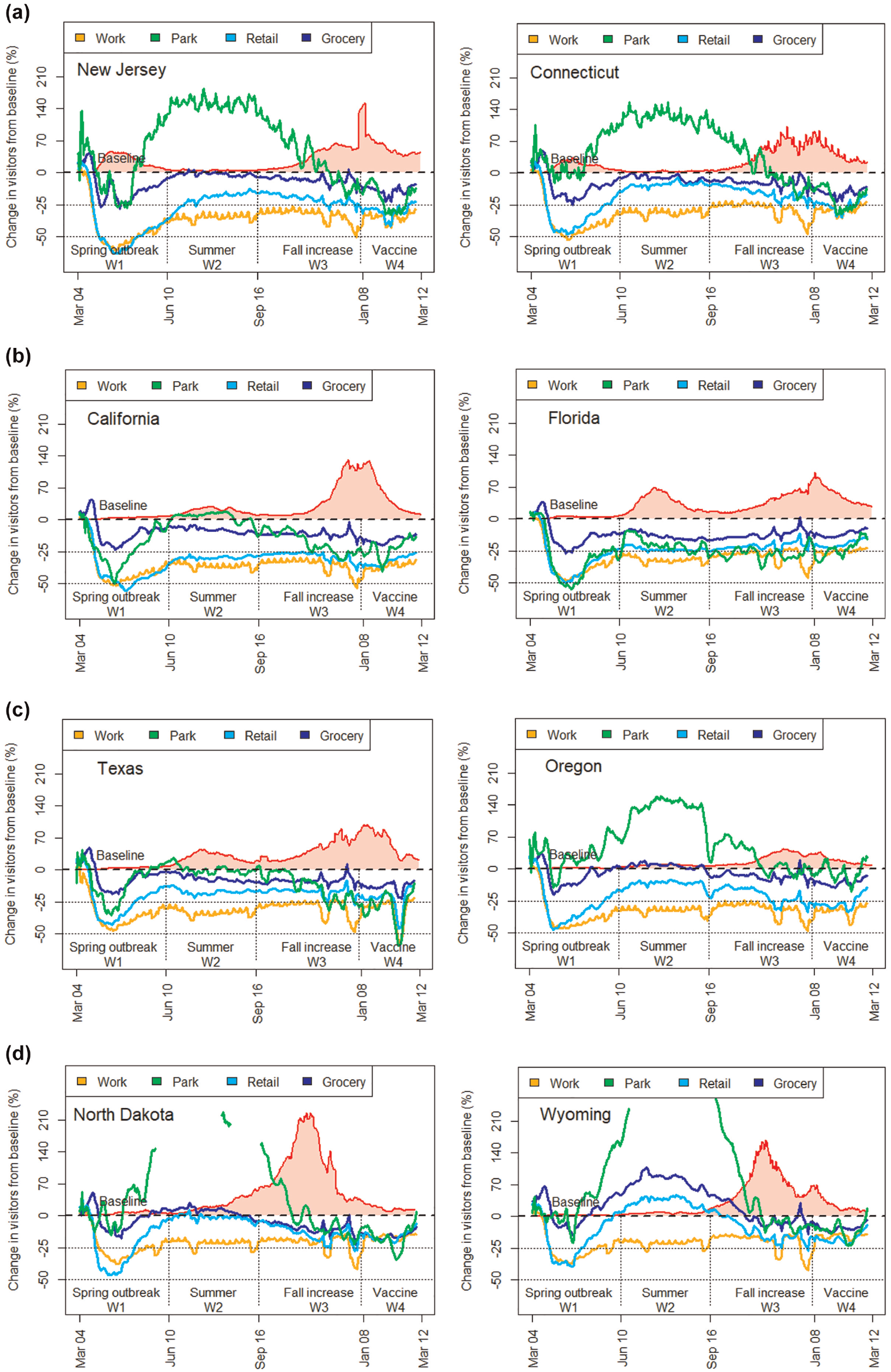
Changes in number of activity visits versus baseline travel and daily new cases per 100,000 population (red shaded area) in representative states per cluster: (a) small urban states, (b) large urban states, (c) urban–rural mixed states, and (d) rural states.

Figure 7 shows the changes in number of activity visits for two representative states for each of the four clusters. The figure also shows the daily new infections per 100,000 population during the same period (red shaded area). In general, an initial sharp decline is observed for the number of all activity visits in all states during the spring outbreak period (window 1). This is because most states issued their first lockdown instructions during this time. This decline was followed by a rise after the lockdown period (appears as a “V” shape in the diagram). Among the four types of activity visits, the number of workplace, and retail and recreation visits declined more and remain lower throughout the year. On the other hand, the number of grocery and park visits increased after the initial decline and approached the baseline. The number of park visits decreased significantly during the holiday seasons in fall 2020 when the infection rate spiked.

Noticeably, there was a smaller reduction in the number of workplace visits in rural states (cluster 4) compared with their urban counterparts, whereas there was a higher reduction in the number of grocery and retail visits in urban states (small, large, and mixed) compared with their rural counterparts (cluster 2, large urban states, had the largest reduction in the number of grocery visits among the four clusters). On the other hand, the number of grocery visits in rural states did not decline much from the baseline and remained close to the baseline throughout the year (in fact, the number of grocery visits in Wyoming exceeded the baseline during the summer period). With the rise of infections during the fall, the number of grocery visits declined. Noticeably, there was a large increase in the number of park visits in small urban states during the summer, as there was in rural states. This rise may in part be attributed to (a) a lower infection rate in summer 2020 and (b) people increasingly opting to gather outdoors because of social distancing guidelines. Note that because of user privacy reasons, Google mobility data does not report visitor counts when the number of participants on a certain day in a certain area falls below a certain number of a small number. On those days, the reported data contain NA (not applicable/missing) markers. For some rural states, for example, North Dakota and Wyoming, this happened on some consecutive dates; therefore, the plot lines break on those days (Figure 7d).

Changes in Trips by Distance

Changes in activity participation contributed to changes in the number of trips. Based on the BTS 2020 data, Figure 8 shows the percentage changes in the number of trips throughout the year with respect to the same day in the previous year. Trips were categorized into four types based on their distance: (a) short-distance trips (below 5 mi); (b) average commute distance (5–25 mi); (c) long commute distance (25–50 mi); and (d) long-distance trips (above 50 mi). The figure also shows the percentage changes in the number of people staying at home compared with the previous year (the shaded area), which was reported as positive because more people stayed at home in 2020 compared with 2019.

Figure 8.

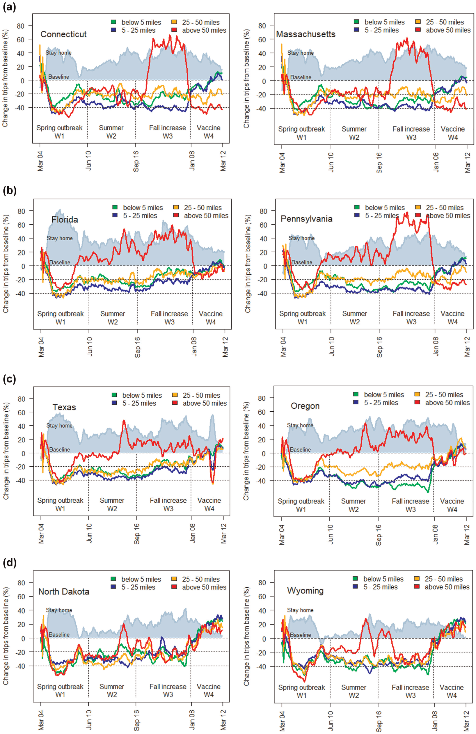
Changes in number of trips with respect to baseline travel and changes in the fraction of people staying at home in representative states per cluster: (a) small urban states, (b) large urban states, (c) urban–rural mixed states, and (d) rural states. Note: W = window. Source: Bureau of Transportation Statistics (21).

Similar to the changes in the number of activity visits, a V-shaped pattern was also observed in the changes in number of trips during the initial outbreak period. This means numbers of trips in all distance categories reduced considerably during the lockdown period followed by an increase after the lockdown. The levels were then stable for the remainder of the year except for long-distance trips. The number of long-distance trips increased during the summer and fall, and then decreased after the holidays. Potential reasons for this pattern include the following: (a) vacation trips in private vehicles increased because of cabin fever (people fed up of being at home all the time); (b) business travel and some commute travel increased in the fall because of a decrease in unemployment; and (c) vacation trips increased because of the effect of family gatherings as the Thanksgiving and Christmas holidays approached. Among all trip distance categories, trips under 25 mi showed the greatest reduction. Notably, all trip lengths increased in frequency in the first few months of 2021.

In the small urban states (sampled by Connecticut and Massachusetts) there was a large rise in the number of long-distance trips during fall 2020 compared with the same period in 2019, followed by a sharp decline at the start of the new year 2021. Interestingly, in the mixed states (cluster 3) and rural states (cluster 4), there was a progressive rise in numbers of trips in the short- and long-distance categories during the first few weeks of 2021. With regard to the fraction of people staying at home during the pandemic (the shaded area in the diagrams), a higher fraction of urban people stayed at home compared with their rural counterparts.

Changes in PMT and VMT

We examined how the changes in number of visits to activity locations during the pandemic were associated with changes in PMT (average distance traveled per person per day) and how the association varies across urban and rural counties in the U.S.A. Figure 9 shows the distribution by county based on changes in the number of nonworkplace visits (x-axis) and changes in the number of workplace visits (y-axis). The counties are color coded according to the degree of PMT: green indicates low PMT whereas red denotes high PMT. Low and high values are determined with respect to the U.S. median value for PMT over the one-year pandemic period. The four quadrants were determined depending on the median values across the respective axes. The fraction of counties in high and low PMT categories is reported in the respective quadrants. These features are shown for both urban counties (Figure 9a) and rural counties (Figure 9b).

Figure 9.

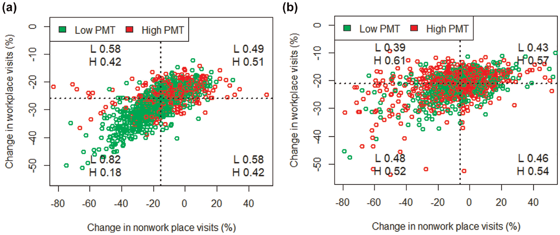
Distribution of counties based on changes in nonworkplace and workplace visits by PMT: (a) urban counties in the U.S.A. and (b) rural counties in the U.S.A.

Counties that were considered urban showed a notably different relationship between the number of work and nonwork visits, and PMT compared with rural counties. For example, in urban counties, the lower the number of work and nonwork visits (lower-left quadrant in Figure 9a), the lower the PMT (82% of counties have low PMT). On the contrary, in rural counties, a lower number of work and nonwork visits corresponded to higher PMT values (in the lower-left quadrant, 52% of counties have high PMT, Figure 9b). A lower number of nonwork visits and a higher number of work visits contributed to higher PMT values (upper-left quadrant in Figure 9b). This means, in both cases, a lower number of nonwork visits was associated with a higher PMT value, which indicates that the reduction in the number of nonwork visits does not necessarily reduce the average distance traveled per person in a county unless the work trips, nonwork trips, or both, are associated with shorter travel distances.

It was anticipated that a reduction in the number of workplace visits and an increase in working from home may have involved less distance traveled in an area because working from home does not involve commuting. To examine this effect, quantile boxplots were constructed, as shown in Figure 10, to depict the corresponding PMT in counties within a specified range of the percentage change in workplace visits. Here, the counties are split into groups based on quartile values, with Q1 denoting counties below the 25th percentile value of the percentage change in work visits, Q2 denoting counties above the 25th percentile but below the 50th percentile, and so on. It is observed that counties with fewer workplace visits had lower PMT, because the median values (the central line inside the box) increased in higher quartile boxes (Figure 10a). However, this relationship did not hold for rural counties. In rural areas, higher PMT was observed for lower quantile values of workplace visits (Figure 10b). The higher number of nonwork activity visits and longer travel distance to access those facilities in rural areas might increase the PMT despite the reduction in number of workplace visits.

Figure 10.

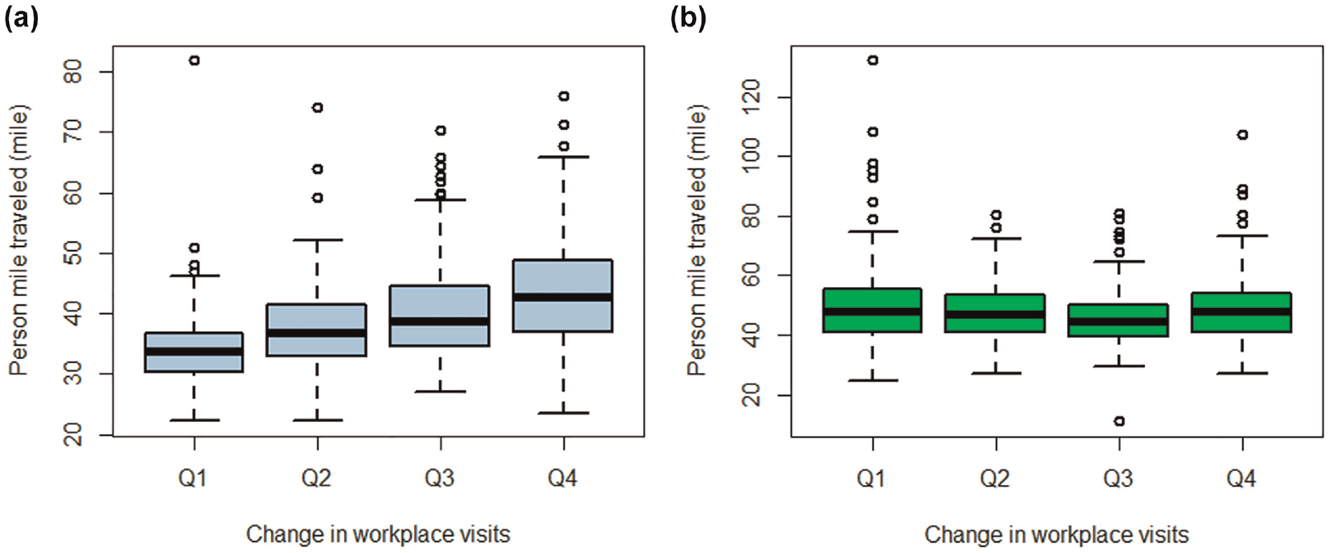
Relationship between percentage change in workplace visits and person-miles traveled: (a) urban counties in the U.S.A. and (b) rural counties in the U.S.A.

We next observe how changes in the number of activity visits, as well as trips, are reflected in the changes in VMT during the one-year pandemic period. Figure 11 shows the percentage changes in VMT for every month from March 2020 to March 2021 with respect to the same month of the previous year. The changes in VMT are shown for the selected three sample states for each of the four clusters. Similar to the changes in the number of activity visits and trips, a V-shaped pattern was observed for changes in VMT during the spring outbreak period. This means that VMT dropped in April and increased again after the lockdown period from mid-May, and then progressed steadily throughout the year with a slight increase in the summer and fall. The variations are observed to be more consistent in the selected urban states (small and large) whereas a lot more variation is noticeable in the mixed and rural states. In general, there was a lower reduction in VMT in rural states compared with their urban counterparts (the reduction was above 40% in rural states, whereas in urban states the reduction went far below 40% in all urban categories). Additionally, the reduction from the baseline in rural states is smaller compared with urban states (the gap between the baseline and the VMT trend lines for different states). Furthermore, from February 2021, VMT started to recover, particularly in urban states, possibly because of the start of the vaccination efforts. However, with the lower vaccination coverage in rural areas (39% versus 46% reported in Murthy et al. [ 30 ]), the return to normal VMT in rural states during that window was rather slow compared with urban states (for instance, urban states crossed the baseline halfway through the window, whereas rural states remained below the baseline).

Figure 11.

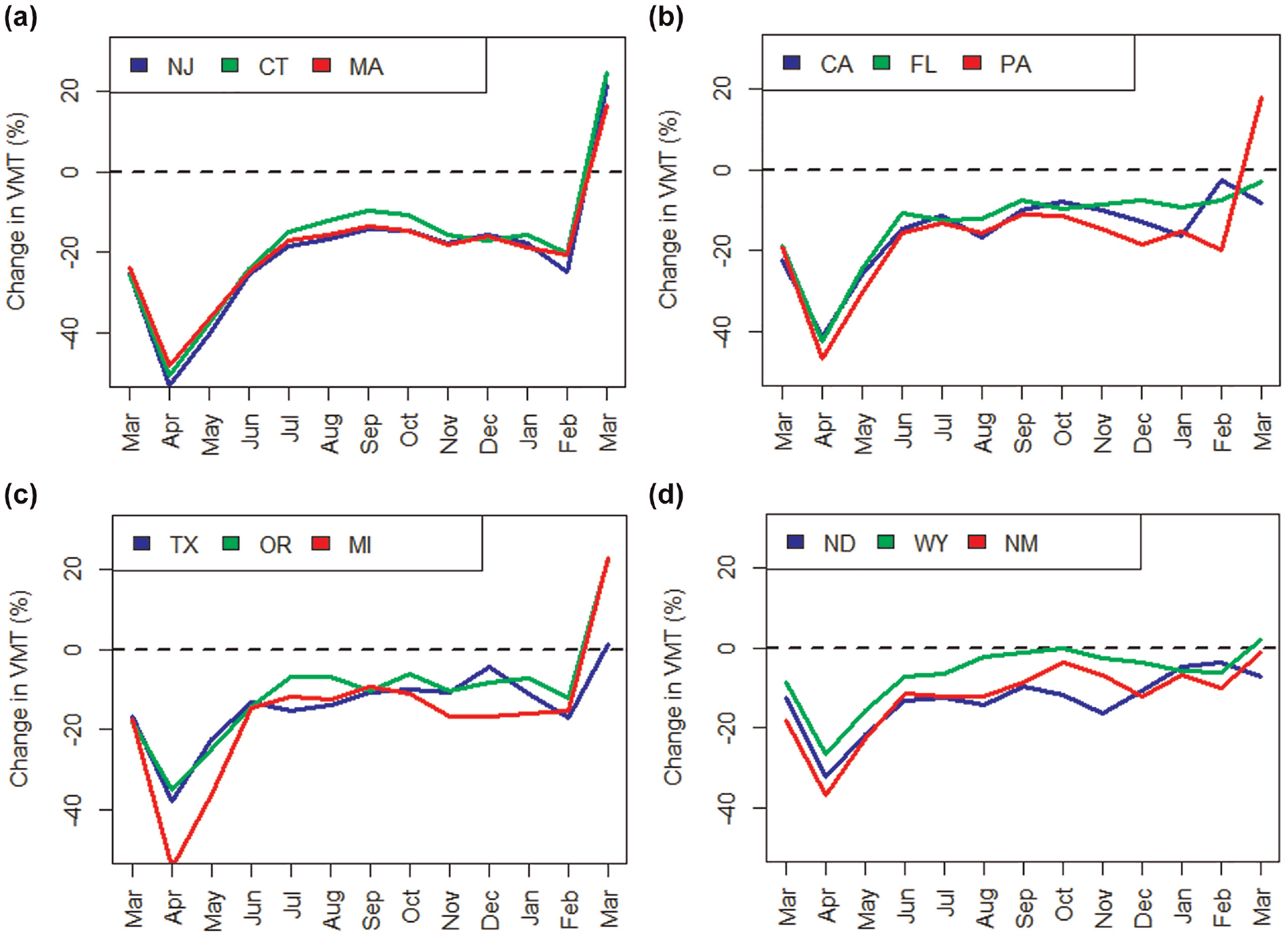
Changes in VMT with respect to the previous year in representative states per cluster: (a) small urban states, (b) large urban states, (c) urban–rural mixed states, and (d) rural states.

Changes in Mode Usage

The changes in mode usage behavior indicate changes in peoples’ travel choices during the pandemic. To show changes in mode usage behavior, we used the COVID Future Wave1 Survey data ( 24 ) conducted from April 14 to October 14, 2020, in which respondents were asked to report their frequency of mode usage before and during the pandemic (last seven days of the survey day). The stacked chart in Figure 12 represents the frequency of mode usage considering all four cluster states. Four frequency categories were considered based on a decreasing degree of usage: “Everyday,”“Few times a week,”“Rarely,” and “Never.”

Figure 12.

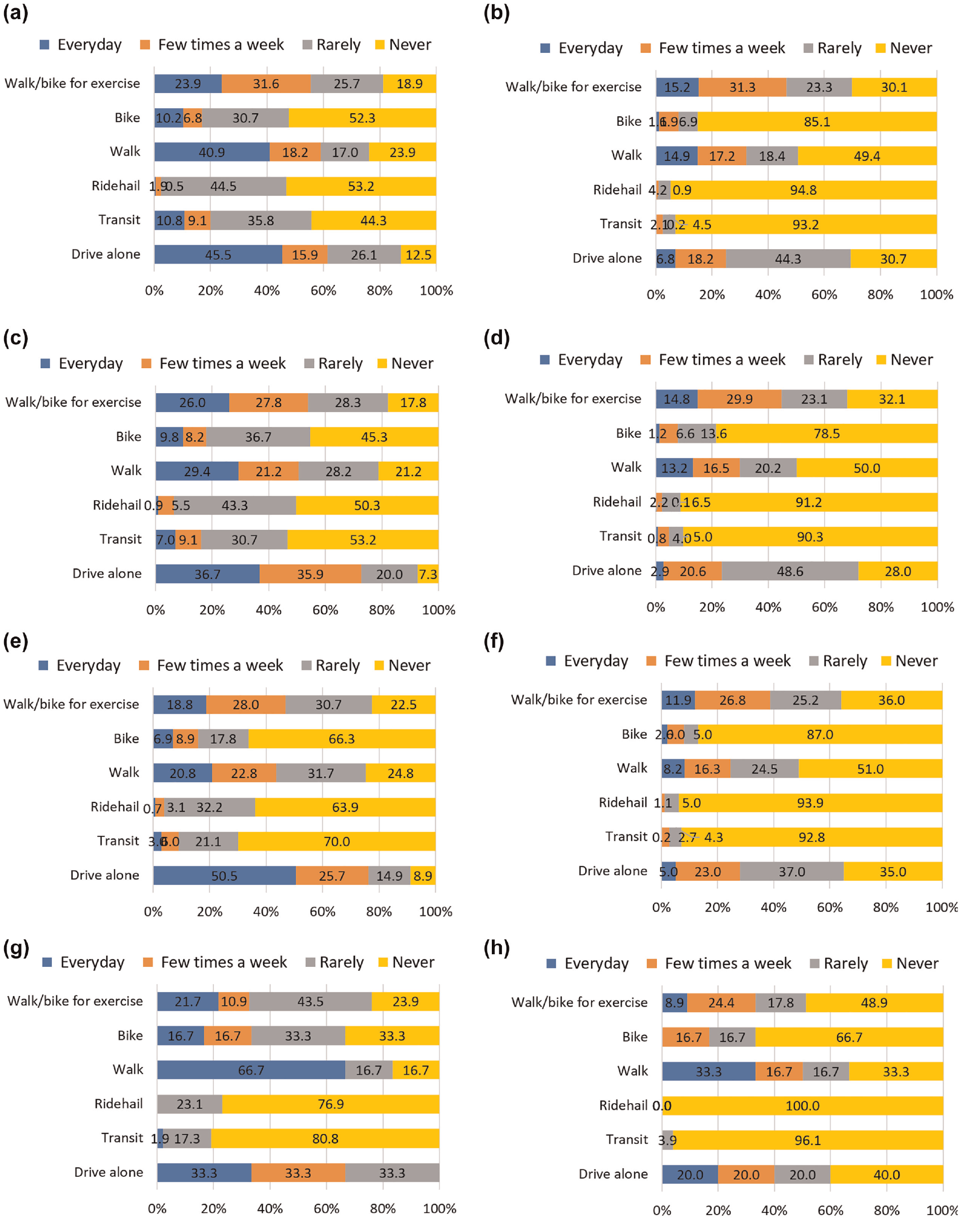
Frequency of mode usage before and during the pandemic across states in four identified clusters: (a) small urban states (before pandemic), (b) small urban states (during pandemic), (c) large urban states (before pandemic), (d) large urban states (during pandemic), (e) urban–rural mixed states (before pandemic), (f) urban–rural mixed states (during pandemic), (g) rural states (before pandemic), and (h) rural states (during pandemic).

Because the number of trips decreased during the pandemic, there were reductions in frequency for almost all modes, predominantly for ride-hailing and transit (the length of “Never” bars are longer in Figure 12, b, d, f, and h ). The frequency of ride-hailing and transit use plummeted, in part because people wished to avoid the risk of exposure to the virus while traveling with strangers. The decrease in the frequency of walk/bike usage for exercise was small compared with other mode usage frequencies. The frequency of daily driving reduced more in urban states compared with rural states.

Conclusions

In this exploratory study, we examined how the adoption of telecommuting, and travel behavior varied across different geographies in the U.S.A. over one full year of the pandemic (March 4, 2020 to March 12, 2021) based on a range of aggregate and disaggregate data sources. To explore the spatial variation of the impact of the pandemic across 50 U.S. states systematically, we applied a K-means clustering technique to identify clusters of states with similar geographic characteristics based on four attributes: the fraction of urban counties; the fraction of population in urban counties; the fraction of area occupied by urban counties; and the fraction of people working from home during the study period. Four clusters were identified: 6 small urban states; 8 large urban states; 18 urban–rural mixed states; and 17 rural states. For each cluster identified, three representative states were selected to explore the impact of the pandemic on the adoption of telecommuting, and travel behavior during the study period. The impact was examined based on a comprehensive descriptive analysis and visual trends of a range of activity travel analytics. Major findings of this study are summarized below:

(a) Findings on changes in telecommuting behavior

About one-third of the U.S. workforce worked from home during the pandemic, which was about six times higher than before the pandemic. More people worked from home in urban states compared with rural states. Among urban states, the largest share of working from home was found in small urban states.

A higher percentage of people working from home in a state corresponded to a greater reduction in the number of workplace visits in that state during the pandemic. The largest reduction in the number of workplace visits was in small urban states followed by large urban states and urban–rural mixed states.

Nearly 35% of households across the U.S.A. saw at least one member substituting their in-person work with telework. The substitution rate in small urban states and rural states were above and below the U.S. national average, respectively.

In both urban and rural states, a higher fraction of workers who worked from home during the pandemic reported their preference to continue doing so even after the threat from the pandemic lessened.

(b) Findings on changes in activity travel behavior

The general trend in changes in the number of activity visits indicated a sharp decline during the initial outbreak period followed by an increase after the lockdown period (a V-shape in the trend plots) and then stable progress throughout the year with fewer visits with respect to the baseline. There were smaller reductions in the number of both workplace and nonworkplace visits in rural states compared with urban states. There was a higher increase in the number of park visits in summer in both rural states and small urban states. This decreased in the fall after the holiday season.

Long-distance trips increased during the summer and fall and then decreased after the holidays. Compared with urban states, the changing pattern of trips in rural states was different. There was a progressive rise in all trip distance lengths during the first few months of 2021 in both urban–rural mixed states and rural states. In urban states, a higher fraction of people stayed at home compared with their rural counterparts.

In urban counties, fewer work and nonwork visits led to a decrease in PMT whereas in rural counties the opposite result was observed (fewer work and nonwork visits were associated with an increase in PMT).

Because of a reduction in the number of activity visits and trips, VMT dropped during the lockdown period but began to increase after the lockdown starting in mid-May. In general, there was a lower reduction in VMT in rural states compared with urban states.

The frequency of ride-hailing and transit usage reduced drastically during the pandemic in both urban and rural states. The frequency of daily driving reduced more in urban states compared with rural states.

With regard to the changes in telecommuting and travel behavior, the critical question is whether the changes have persisted in the long term. By analyzing disaggregate-level data, we observed that a higher fraction of workers preferred to continue working from home after the pandemic ended. Previous studies also suggested the continuation of working from home post-pandemic ( 10 , 31 , 32 ). Recently, a San Francisco-based IT company adopted three options for its employees: fully remote, flex, and traditional ( 33 ). In the flex option, employees commute to the office between one and three days per week for meetings, presentations, and collaborations, and work from home on the remaining days. It is anticipated that similar policies could possibly be adopted by other companies in the near future.

If telecommuting continues at a pandemic level or in a hybrid manner, there may be some advantages and challenges associated with this unconventional work arrangement that need to be addressed in relevant policies. For example, telecommuting may be good for the negative effects of transportation, because during the pandemic there were fewer work trips, a reduction in heavy peak hour flow, and fewer miles traveled, resulting in less air pollution ( 16 ). Therefore, policies that promote telecommuting can be encouraged. However, the impact of telecommuting on business is uncertain. There may be an impact on work productivity for some businesses. Moreover, if there are fewer workers who are commuting, this may reduce nonwork activities associated with commuting. For example, if people work from home more, it may affect daytime business because they will not be at conventional activity centers as frequently. In addition, a reduction in commuting may have a negative impact on public transit ridership. Public transit operators may need to restructure their services or introduce new technologies to accommodate demand.

Working from home may likely change the demand for both commercial and residential space requirements. For example, employers may reduce their commercial spaces whereas employees may need to accommodate a dedicated workspace in their existing home. Employees may prefer to move from urban residences to outlying areas to gain increased space for working from home. This may raise demand for larger homes in suburban areas and, thus, may have an impact on the housing market. Recent house price increases may be an early sign of this ( 34 ). The ramifications for local, regional, and state land-use policies as well as transportation because of these changes in residential location choices are uncertain and complicated. There are likely equity issues in the adoption of working from home. We observed that it will not be as easy for low-income workers and people living in rural counties to adopt this working arrangement because of the nature of their jobs. Policies may need to evolve to consider safe and easy access to jobs, transportation facilities, and healthcare systems. Considering all these aspects, it appears that the post-pandemic workplace experience may be different from that in the pre-pandemic era, with greater accommodation of working from home (telecommuting), accompanied by other changes in work and nonwork activity travel arrangements. Consequently, relevant land-use and transportation policies need to be considered to embrace these challenges.

During our study time window, most Americans were not yet fully vaccinated against COVID-19. Therefore, we could not capture the true impact of vaccination on peoples’ activity travel schedules. Our future research interest is to extend the study time window and to explore the impact of vaccination on peoples’ actions and travel choices. In summary, the study’s findings suggest that there are both some similarities and differences in the changing patterns of telecommuting and activity travel behavior between urban and rural geographies observed during the COVID-19 pandemic. These findings are expected to provide valuable insights for policies that influence telecommuting, transportation, and land-use issues, and for the assessment of geographic variations in the adoption of telecommuting, participation in activity travel, and a broad range of associated impacts. The insights into regional variations will also provide guidance for future pandemic-related policy initiatives, such as response mechanisms and resource allocation.

Footnotes

Author Contributions

The authors confirm contribution to the paper as follows: study conception and design: R. Rafiq, M. G. McNally; data collection: Y. S. Uddin, R. Rafiq; analysis and interpretation of results: R. Rafiq, M. G. McNally, Y. S. Uddin; draft manuscript preparation: R. Rafiq, M. G. McNally, Y. S. Uddin. All authors reviewed the results and approved the final version of the manuscript.

Declaration of Conflicting Interests

The author(s) declared no potential conflicts of interest with respect to the research, authorship, and/or publication of this article.

Funding

The author(s) received no financial support for the research, authorship, and/or publication of this article.

ORCID iDs

Rezwana Rafiq

Michael G. McNally

Md Yusuf Sarwar Uddin

References

Brynjolfsson

Horton

J. J.

Ozimek

Rock

Sharma

TuYe

H. Y

. COVID-19 and Remote Work: An Early Look at US Data. Working Paper no. 27344. National Bureau of Economic Research, Cambridge, MA, 2020.

Holshue

M. L.

DeBolt

Lindquist

Lofy

K. H.

Wiesman

Bruce

Pillai

S. K.

, et al. First Case of 2019 Novel Coronavirus in the United States. New England Journal of Medicine, Vol. 382, 2020, pp. 929–936.

Centers for Disease Control & Prevention. Meat and Poultry Processing Workers and Employers. https://www.cdc.gov/coronavirus/2019-ncov/community/organizations/meat-poultry-processing-workers-employers.html. Accessed June 15, 2021.

Andersen

L.M.

Harden

S. R.

Sugg

M. M.

Runkle

J. D.

Lundquist

T. E.

Analyzing the Spatial Determinants of Local Covid-19 Transmission in the United States. Science of the Total Environment, Vol. 754, 2021, Article 142396.

Paul

Arif

A. A.

Adeyemi

Ghosh

Han

Progression of COVID-19 from Urban to Rural Areas in the United States: A Spatiotemporal Analysis of Prevalence Rates. The Journal of Rural Health, Vol. 36, No. 4, 2020, pp. 591–601.

Karim

S. A.

Chen

H. F.

Deaths from COVID-19 in Rural, Micropolitan, and Metropolitan Areas: A County-Level Comparison. The Journal of Rural Health, Vol. 37, No. 1, 2021, pp. 124–132.

Rafiq

Ahmed

Uddin

M. Y. S.

Structural Modeling of COVID-19 Spread in Relation to Human Mobility. Transportation Research Interdisciplinary Perspectives, Vol. 13, 2022, Article 100528.

Mueller

J. T.

McConnell

Burow

P. B.

Pofahl

Merdjanoff

A. A.

Farrell

Impacts of the COVID-19 Pandemic on Rural America. Proceedings of the National Academy of Sciences, Vol. 118, No. 1, 2021, Article 2019378118.

Callaghan

Lueck

J. A.

Trujillo

K. L.

Ferdinand

A. O.

Rural and Urban Differences in COVID-19 Prevention Behaviors. The Journal of Rural Health, Vol. 37, No. 2, 2021, pp. 287–295.

10.

Beck

M. J.

Hensher

D. A.

Insights into the Impact of COVID-19 on Household Travel and Activities in Australia – The Early Days of Easing Restrictions. Transport Policy, Vol. 99, 2020, pp. 95–119.

11.

Astroza

Tirachini

Hurtubia

Carrasco

J. A.

Guevara

Munizaga

Figueroa

Torres

Mobility Changes, Teleworking, and Remote Communication during the COVID-19 Pandemic in Chile. Transport Findings, 2020, pp. 1–12. https://doi.org/10.32866/001c.13489.

12.

Music

Charlebois

Toole

Large

Telecommuting and Food E-Commerce: Socially Sustainable Practices during the COVID-19 Pandemic in Canada. Transportation Research Interdisciplinary Perspectives, Vol. 13, 2022, Article 100513.

13.

De Haas

Faber

Hamersma

How COVID-19 and the Dutch “Intelligent Lockdown” Change Activities, Work and Travel Behaviour: Evidence from Longitudinal Data in The Netherlands. Transportation Research Interdisciplinary Perspectives, Vol. 6, 2020, Article 100150.

14.

Wang

Ozbilen

Synergistic and Threshold Effects of Telework and Residential Location Choice on Travel Time Allocation. Sustainable Cities and Society, Vol. 63, 2020, Article 102468.

15.

Shamshiripour

Rahimi

Shabanpour

Mohammadian

A. K.

How is COVID-19 Reshaping Activity-Travel Behavior? Evidence from a Comprehensive Survey in Chicago. Transportation Research Interdisciplinary Perspectives, Vol. 7, 2020, Article 100216.

16.

Rafiq

McNally

M. G.

Uddin

Y. S.

Ahmed

Impact of Working from Home on Activity-Travel Behavior during the COVID-19 Pandemic: An Aggregate Structural Analysis. Transportation Research Part A: Policy and Practice, Vol. 159, 2022, pp. 35–54.

17.

McNally

M. G.

Rafiq

Uddin

Y. S.

Impacts of the COVID-19 Pandemic on Telecommuting and Travel. In Pandemic in the Metropolis: Transportation Impacts and Recovery ( Loukaitou-Sideris

Bayen

A. M.

Circella

Jayakrishnan

, eds.), Springer, Switzerland, 2022.

18.

The New York Times. Coronavirus (COVID-19) Data in the United States. https://github.com/nytimes/covid-19-data. Accessed February 1, 2021.

19.

Maryland Transportation Institute. University of Maryland COVID-19 Impact Analysis Platform. https://data.covid.umd.edu. Accessed February 1, 2021.

20.

Google LLC. Google COVID-19 Community Mobility Reports. https://www.google.com/covid19/mobility/. Accessed February 1, 2021.

21.

Bureau of Transportation Statistics. Trips by Distance. https://data.bts.gov/Research-and-Statistics/Trips-by-Distance/w96p-f2qv. Accessed March 25, 2021.

22.

Federal Highway Administration (2019–2021). Traffic Volume Trends. Office of Highway Policy Information. https://www.fhwa.dot.gov/policyinformation/travel_monitoring/tvt.cfm. Accessed June 1, 2021.

23.

U.S. Census Bureau (2020–2021). Measuring Household Experiences during the Coronavirus Pandemic. Household Pulse Survey. https://www.census.gov/programs-surveys/household-pulse-survey/datasets.html. Accessed March 26, 2021.

24.

Salon

Wigginton

C. M.

da Silva Denise

Rishabh

Ali

Ehsan

Laura

, et al. COVID Future Wave 1 Survey Data, Version 1.0.0. https://doi.org/10.48349/ASU/QO7BTC. Accessed March 26, 2021.

25.

Ingram

D. D.

Franco

S. J.

2013 NCHS Urban–Rural Classification Scheme for Counties. Vital Health Statistics, Vol. 2, No. 166, 2014, pp. 1–73.

26.

Hartigan

J. A.

Wong

M. A.

Algorithm AS 136: A K-Means Clustering Algorithm. Journal of the Royal Statistical Society. Series C (Applied Statistics), Vol. 28, No. 1, 1979, pp. 100–108.

27.

U.S. Census Bureau. 2014–2018 American Community Survey 5-Year Estimates. 2018. https://www.census.gov/programs-surveys/acs/news/data-releases/2018/release.html. Accessed November 23, 2020.

28.

Brooks

M. M.

Mueller

J. T.

Thiede

B. C.

Rural–Urban Differences in the Labor-Force Impacts of COVID-19 in the United States. Socius: Social Research in Dynamic World, Vol. 7, 2021, Article 23780231211022094.

29.

Vincent

. Will Employers Ditch Offices in Favor of Working from Home? Los Angeles Times. https://www.latimes.com/business/story/2021-08-12/office-rentals-shrink-as-tenant-employees-work-from-home. Accessed August 16, 2021.

30.

Murthy

B. P.

Sterrett

Weller

Zell

Reynolds

Toblin

R. L.

Murthy

, et al. Disparities in COVID-19 Vaccination Coverage between Urban and Rural Counties – United States, December 14, 2020–April 10, 2021. MMWR Morbidity and Mortality Weekly Report, Vol. 70, 2021, pp. 759–764.

31.

Amekudzi-Kennedy

Labi

Woodall

Chester

Singh

Reflections on Pandemics, Civil Infrastructure and Sustainable Development: Five Lessons from COVID-19 through the Lens of Transportation. Preprints, 2020. https://doi.org/10.20944/preprints202004.0047.v1.

32.

Keller

Top 500 Design Firms: Designing for the New Normal. Engineering News-Record. https://www.enr.com/articles/51631-top-500-design-firms-designing-for-the-new-normal. Accessed April 24, 2021.

33.

Naylor

. How Will Remote Work beyond the Pandemic Impact the Bay Area?https://www.ktvu.com/news/how-will-remote-work-beyond-the-pandemic-impact-the-bay-area. Accessed June 15, 2021.

34.

Giammona

U.S. Housing Prices Jump the Most in More Than 30 Years. https://www.dailybulletin.com/2021/06/29/u-s-housing-prices-jump-the-most-in-more-than-three-decades/. Accessed June 29, 2021.