Overfitting Prevention in Accident Prediction Models: Bayesian Regularization of Artificial Neural Networks

Abstract

In the present paper, we implemented the Bayesian regularization (BR) backpropagation algorithm for calibrating an artificial neural network (ANN) as an accident prediction model (APM) to be used on Italian four-lane divided roads. We chose the BR-ANN since it efficiently allows for dealing with small sample size and avoiding overfitting issues by adding a regularization term in the objective function to be minimized during training. Moreover, BR-ANNs are sparsely employed in road safety analyses, and their peculiarities deserve to be emphasized. In our work, the BR-ANN aims to predict the number of fatal and injury (FI) crashes across 236 road elements, for a total length of 78 km. The input features are road element length, horizontal and vertical alignment, cross-section geometry, operating speed, traffic flow, sight distance, and road area type (i.e., a categorical predictor accounting for the potential influence of merge and diverge influence areas). Training and test phases of the BR-ANN have been evaluated by determination coefficient (R²), root mean square error (RMSE), overfitting ratio (OR), scatterplots, residuals analysis, and by the same ANN architecture trained with the gradient descent (GD) with momentum and adaptive learning rate backpropagation algorithm (GD-ANN). Results demonstrate that the BR-ANN markedly outperforms the GD-ANN, which suffers severe overfitting issues. Furthermore, BR-ANN does not overfit data (OR close to the unity), reports a satisfactory R² (0.726), and shows a Gaussian residual distribution with zero mean. Therefore, road authorities could consider regularized ANNs for performing appropriate safety analyses, especially when dealing with small road sample sizes.

Keywords

accident prediction models crash analysis artificial neural networks Bayesian regularization backpropagation algorithm overfitting Issue road safety four-lane divided roads

The latest World Health Organization report on road safety states that more than 1.35 million people die each year from causes related to road accidents ( 1 ). Specifically, crash injuries represent the leading causes of death for children and young adults aged between 5 and 29 years. These aspects lead to an urgent call to the academic community to develop innovative and reliable solutions to prevent as many severe road accidents as possible. As such, the road safety level is widely investigated from several perspectives, which can be summarized as the following fields of research: crash severity prediction ( 2 – 4 ), detection of real-time crashes ( 5 , 6 ), detection of road blackspots ( 7 , 8 ), and crash frequency prediction ( 9 – 11 ). In the present paper, we refer to the latter aspect.

Literature offers two modeling approaches for predicting the number of crashes on a road element in a time frame: the statistical parametric approach and the data-driven nonparametric approach ( 12 , 13 ). Ordinarily, statistical parametric accident prediction models (APMs) employ generalized linear models constrained by the leading hypothesis that crash frequency behaves like a random variable distributed according to a negative binomial distribution ( 10 , 14 , 15 ). Such a hypothesis can be validated empirically or by statistical tests, such as the likelihood ratio test ( 16 ). Unfortunately, these a priori assumptions cannot invariably be proved, and there are no theoretical rules that endorse their validity. As a result, the risk of biased predictions may be significant.

To avoid such issues, many studies have experimented with data-driven nonparametric models, such as machine learning algorithms (MLAs) or deep learning algorithms (DLAs), demonstrating that the performance of the statistical parametric modeling approach can be improved on ( 17 – 20 ). These algorithms do not assume a specific statistical distribution linked to the output target to be predicted. Moreover, they can interpret any relationship between input features and output target and handle numerical, categorical, ordinal, and missing data. Also, potential highly correlated inputs can be considered in the modeling since MLAs and DLAs can emphasize the relationships linking the most influential inputs with the output and, at the same time, moderate the relations of redundant and unuseful ones. Specifically, some researchers attempted to model crash frequency and crash severity by exploiting the capabilities of artificial neural networks (ANNs), showing that their performance is higher than other MLAs ( 4 , 5 , 19 , 21 ). Nevertheless, the use of ANNs requires complex hyperparameter tuning and the risk of facing overfitting issues. Indeed, as the name suggests, data-driven models generally require a significant amount of data since they tend to suffer from severe overfitting issues if trained with a small training set.

Unfortunately, in certain countries such as Italy, the availability of large data sets is a significant concern in road safety analyses, especially for regional road authorities. Accordingly, the calibration of reliable data-driven APMs is not often an easy task, and such a modeling approach could provide unreliable prediction if not regularized with appropriate techniques ( 22 , 23 ). As a regularization method, the BR backpropagation algorithm allows for avoiding overfitting issues in ANNs, even when the training set is limited. Indeed, by adding a regularization term in the objective function to be optimized during the learning process, the BR-ANN can prune insignificant synaptic links between artificial neurons and improve its generalization capabilities on new data. Nonetheless, BR-ANN has been sparsely implemented in road safety analyses to the best of our knowledge. Specifically, we identified just one study concerning a classification task ( 24 ), that is, for modeling the crash occurrence as a categorical binary output, and two works on regression tasks ( 25 , 26 ), that is, for predicting the crash frequency as numerical output.

Schlögl et al. ( 24 ) implemented a BR-ANN along with 10 additional data-driven algorithms for predicting the crash occurrence across the whole freeway network of Austria. The authors could handle a high-resolution database with about 4500 crash occurrences and more than 300 million records of non-crash occurrences. Once the issue of data imbalance ( 2 ) had been solved with appropriate sampling techniques, the authors trained the data-driven algorithms; it was found that XGBoost outperforms the other algorithms, exhibiting an accuracy of about 90%. However, albeit with the use of a high-resolution data set with millions of records, most of the other algorithms (including the BR-ANN) showed a false positive rate of nearly 40% to 50%, and an area under the curve (AUC) slightly higher than 0.6; this may indicate under- or overfitted models, unable to predict crash occurrence on new data correctly.

Chakraborty et al. ( 25 ) attempted to model pedestrian crashes at Indian urban intersections. The authors proposed some crash prediction models based on ANNs. Relying on three different sets of activation functions and four learning algorithms for ANNs, they found that using hyperbolic tangent sigmoid functions along with BR-ANNs outperforms all the other models, providing the highest predictive performance in pedestrian crash occurrences and the best OR (about 1). Nonetheless, the R² seems low across all algorithms (about 0.3–0.4), indicating that the fitting process may have experienced some challenges.

Finally, in Xie et al. ( 26 ), the authors focused on implementing a negative binomial regression, a multilayer perceptron ANN, and a BR-ANN for predicting motor vehicles across rural frontage roads in Texas. First, the authors acknowledged the issue of overfitting when using ANNs, and stated that BR-ANN might be beneficial in overcoming this task. It was found that BR-ANN outperforms the other models in predictive performance and can effectively alleviate the overfitting issue without significantly compromising the nonlinear approximation ability.

An additional study related to accident reconstruction has been proposed by Riviere et al. ( 27 ), where the BR-ANN has been efficiently calibrated for modeling and predicting the equivalent energy speed absorbed by vehicles after a crash impact.

Therefore, among the four papers identified and briefly described above, the research of Xie et al. ( 26 ) is the only one that recognizes the problem of overfitting and uses the BR-ANN to overcome it. Therefore, the present study fully supports those findings and aims to provide an additional contribution to this research field. We focus on a different type of infrastructure (i.e., four-lane divided roads), a significantly different context (i.e., Italy), and additional road-related features used as predictors. We undoubtedly recommend the work of Xie et al. ( 26 ) to readers since it is probably the first recognized in the literature to deal with BR-ANN in road safety research for handling overfitting issues.

Considering this, in the present paper, we aim to emphasize the strengths of BR-ANNs, extend their implementation to four-lane divided roads where no studies have been recognized, and evaluate potential deriving benefits in accident data analysis dealing with a small sample size. First, we calibrate a BR-ANN to predict the number of fatal and injury (FI) crashes across 78 km of Italian four-lane divided roads. That BR-ANN attempts to identify a relationship between 10 road-related input features and 3413 FI crashes that occurred between 2015 and 2019, that is, the output targets to be predicted. The learning process is evaluated by the mean squared error (MSE) value during the epochs of training and test. Once trained, we assess the BR-ANN performance by R², root mean square error (RMSE), overfitting ratio (OR), scatterplots, residuals analysis, and comparison with a “traditional” GD-ANN (GD being gradient descent). Finally, the importance of each input feature in predicting the output target is computed and discussed.

Methods

Workflow

The leading phases of the proposed procedure are recapped in Figure 1.

Figure 1.

Workflow of the proposed methodology.

First of all, data concerning the investigated road network were collected and preprocessed to define the homogeneous sections and an appropriate database. Therefore, 236 homogeneous sections were defined, for which 10 explanatory variables (input features) and one dependent variable (output target) were identified. Subsequently, according to a 10-fold cross-validation, the ANN architecture was established, and the BR-ANN and GD-ANN were trained and tested. The ANNs’ performance during epochs was quantified, and their training process evaluated by observing specific plots of characteristic parameters. Goodness-of-fit (i.e., training phase performance) and predictive performance (i.e., test phase performance) were evaluated by the R², RMSE, OR, scatterplots, and residual distribution plots. Supported by the performance obtained, the BR-ANN was trained on all road sections (deployment phase). Finally, the implications of each explanatory variable for the dependent variable were evaluated by the predictor importance parameter.

Artificial Neural Networks

ANNs were devised in the research of McCulloch and Pitts in the early 1940s ( 28 ). The authors outlined the analytical hypotheses for assimilating the biological neural network to a mathematical process. An ANN is an arch and node structure; like the biological neural network, the ANN is structured in layers of artificial neurons interconnected with each other by synaptic links. The architecture of an ANN includes at least three layers: an input layer, a hidden layer, and an output layer. In the input layer, each artificial neuron receives one input feature belonging to a training sample. From the input layer, signals are transferred to the hidden layer. From the latter, the signal is transformed by a transfer function and transferred to the output layer. The output layer consists of a single artificial neuron in regression tasks, whose output signal coincides with the ANN prediction. Finally, it is worth noting that there is a bias neuron in the input and hidden layers, that is, an artificial neuron whose output is always one. Figure 2 shows the ANN scheme implemented in the present research. Such an ANN can also be defined as a multilayer perceptron ANN or feed forward ANN.

Figure 2.

Artificial neural network (ANN) architecture.

In Figure 2, $p_{j}$ are the input features belonging to a road element, $b$ are the biases, $w_{jk}$ are the synaptic weights between input and hidden layers, $b_{j}^{(1)}$ are the synaptic weights relative to the bias of the input layer, $z_{k}$ are the synaptic weights between the hidden and output layers, $b^{(2)}$ is the synaptic weight relative to the bias of the hidden layer, $Σ$ is the summation of signals arriving at each neuron, $f$ and $g$ are the transfer functions, and $\hat{Y_{i}}$ is the prediction made by the ANN.

In the present research, the hyperbolic tangent sigmoid (Equation 1) has been employed as transfer function $f$ in the hidden layer. Such a function can be expressed as

f (x) = \frac{2}{(1 + \exp (- 2 \cdot x))} - 1 .

(1)

As stated, each hidden neuron receives as input $\sum_{j = 1}^{R} w_{kj} \cdot p_{j} + b_{k}^{(1)}$ and reports as output the $f (Σ)$ value. The linear transfer function (Equation 2) has been employed as transfer function $g$ in the output layer:

g (x) = x .

(2)

Accordingly, such a function is a passthrough; the unique output neuron receives as input $\sum_{k = 1}^{K} z_{k} \cdot f (Σ) + b^{(2)}$ , and considers this value as the predicted output target $\hat{Y_{i}}$ . Therefore, starting from a set of input features $p_{j}$ , the present ANN computes the output target $\hat{Y_{i}}$ as follows (Equation 3):

\hat{Y_{i}} = g {\sum_{k = 1}^{K} z_{k} \cdot f (\sum_{j = 1}^{J} w_{jk} \cdot p_{j} + b_{j}^{(1)}) + b^{(2)}} .

(3)

The values of synaptic weights are randomly initialized and each observation belonging to the training set passes through the ANN. Therefore, several predictions are made by the ANN, and an objective function (also called loss function), $F (y)$ , is computed. In regression tasks, it is common to use the MSE as the objective function to be minimized (Equation 4):

F (y) = MSE = \frac{1}{N} \sum_{i = 1}^{N} {[(\hat{Y_{i}} - Y_{i})]}^{2}

(4)

where $\hat{Y_{i}}$ is the predicted value of the target output for the $i$ th element, $Y_{i}$ is the observed value of the target output for the $i$ th element, and $N$ is the size of the training set. Accordingly, by implementing a specific backpropagation algorithm, the values of synaptic weights are adjusted iteratively to minimize the objective function. Readers may find interesting the work of Rumelhart ( 29 ), in which the backpropagation algorithm has been defined and described in detail. GD backpropagation is ordinarily implemented. Generally speaking, the algorithm works by computing the gradient of the objective function concerning each synaptic weight by the chain rule, computing the gradient one layer at a time, and updating synaptic weights backward from the output layer to the input layer. Therefore, the ANN can be optimized by an appropriate number of learning cycles (or epochs).

Bayesian Regularization Backpropagation Algorithm

The Bayesian regularization (BR) process was defined in the 1990s in the works of MacKay ( 23 ). The algorithm is of considerable complexity, and only the key concepts are reported in this section. Readers may find interesting certain detailed implementations of BR-ANNs in references (22, 30 –34). Basically, in the BR process, the objective function of Equation 4 is replaced by (Equation 5):

F (y, W) = α \cdot E_{S} + β \cdot E_{W}

(5)

where $E_{W} = \frac{1}{N} \sum_{j = 1}^{n} w_{j}^{2}$ is the mean of the sum of squares of the network weights and biases, in which $n$ denotes the number of synaptic weights and biases of the ANN. $E_{S}$ is the sum of squared network errors (i.e., the MSE). Both $α$ and $β$ are objective parameters to be estimated during training. In the case that $α >> β$ , the BR-ANN provides negligible errors, and the overfitting issue may persist; on the contrary, if $α << β$ , the BR process provides a significant size reduction of synaptic weights at the expense of higher network errors. Accordingly, the BR backpropagation algorithm aims to calibrate an ANN with the highest performance and the least number of parameters to moderate the issue of overfitting effectively.

In such a modeling framework, synaptic weights are considered as random variables with a Gaussian distribution; this constitutes the prior probability of weights. The use of Gaussian distribution prior is a common practice. Nonetheless, it is worth acknowledging that such a symmetric prior, and the resulting conditioning on a zero-mean distribution, do not appropriately represent the innate symmetry in the signs of the prior weights ( 35 ).

Therefore, by knowing the ANN architecture, the training set, and a set of $α$ , $β$ , it is possible to derive the posterior probability according to Bayes’ theorem. It can be shown ( 30 ) that maximizing the posterior probability (i.e., recognizing the optimal synaptic weights) corresponds to minimizing Equation 5; accordingly, the optimum values of regularization parameters at the minimum point of the posterior density $W^{MP}$ can be computed as

α^{MP} = \frac{N - γ}{2 \cdot E_{S} (W^{MP})}

(6)

β^{MP} = \frac{γ}{2 \cdot E_{w} (W^{MP})}

(7)

γ = n - β^{MP} \cdot tr {(H^{MP})}^{- 1}

(8)

where $H^{MP} = α \nabla^{2} E_{S} + β \nabla^{2} E_{w}$ is the Hessian matrix of the performance function at the minimum point and $γ$ is defined as the effective number of parameters. This parameter identifies the number of synaptic weights in the BR-ANN effectively employed to diminish the objective function. The $γ$ parameter can span from zero to $n$ . Finally, $N$ in Equation 6 represents the number of samples in the training set.

The optimization of $γ$ requires the computation of the Hessian matrix of $F (y, W)$ at the minimum point $W^{MP}$ . Therefore, as proposed by the study of Foresee and Hagan ( 36 ), the Hessian matrix can be estimated by the Gauss–Newton approximation (Equation 9):

H = J^{T} J

(9)

where $J$ is the Jacobian matrix containing the first derivatives of the ANN errors with respect to synaptic weights. Following this approximation, the Levenberg–Marquardt (LM) algorithm ( 37 , 38 ) is implemented for updating synaptic weights and biases according to the following, Equation 10:

W_{k + 1} = W_{k} - {[H + μ I]}^{- 1} \cdot J^{T} .

(10)

where $k$ is the last iteration, $e$ represents the vector of ANN errors (an $i$ th error is defined as $e_{i} = Y_{i} - \hat{Y_{i}}$ ) and $I$ is the identity matrix. The $μ$ parameter is an adaptive value defined as the LM damping factor. After a successful iteration (i.e., when a reduction in the objective function is detected), the LM damping factor $μ$ diminishes its value by multiplying a coefficient $μ_{dec} < 0$ . Conversely, when an iteration is failed, the $μ$ increases its value by multiplying a coefficient 1/ $μ_{dec}$ . Therefore, the performance function is reduced at each algorithm iteration ( 39 ).

ANN Architecture and Modeling Framework

ANN Architecture

The number of artificial neurons in the input layer and output layers is defined. Indeed, for the former, it corresponds with the number of input features associated with each training instance. In addition, there is one bias. There is one artificial neuron in the output layer since the target output is a continuous variable and the task to be performed is a regression.

Accordingly, the relevant aspect of the present ANN architecture is to define the number of hidden layers and the number of artificial neurons belonging to such layers. It is known that an ANN with a single hidden layer can interpret any mathematical function ( 26 ), provided that the artificial neurons in the layer are of a sufficiently high number ( 40 ). Therefore, we employed a single hidden layer in the architecture of the ANNs.

Concerning the number of artificial neurons, it should be noted that a high number may lead to a long training time and a higher risk of overfitting. Nonetheless, the BR-ANN prevents the overfitting issue by pruning the less relevant synaptic weights. Consequently, considering this considerable advantage, one should make sure that the number of neurons in the hidden layer is such as to allow interpreting a complex pattern between input features and output. This aspect is evaluated through some training state plots, that is, graphs in which it is possible to appreciate how the characteristic parameters (gradient, $μ$ , $γ$ ) of the BR-ANN vary epoch by epoch. It seems conceivable to assume that the BR-ANN has sufficient artificial neurons in the hidden layer if such characteristic parameters assume a stable behavior after a certain number of epochs.

Therefore, we implemented several ANN architectures by varying the number of artificial neurons in the hidden layer from 1 to 40. According to a 10-fold cross-validation process ( 41 ), the data set was randomly split into training (80% of samples) and test (20% of samples) sets. For each scenario (i.e., for each implemented architecture), since data for training and testing the ANNs are different and may lead to different outcomes, we trained the ANNs 10 times, observing the average pattern. Therefore, each architecture was trained with the highest degree of generalization, avoiding selectivity bias.

We observed that the BR-ANN assumed a stable behavior during the training phase from 20 artificial neurons onward and provided satisfactory performance. Accordingly, we considered 20 artificial neurons (and one bias) in the hidden layer of the BR-ANN. The GD-ANN was implemented with the same architecture to make a reliable comparison. Figure 3 shows the ANN architecture.

Figure 3.

BR-ANN and GD-ANN architecture.

ANN Modeling Framework

For each training epoch, the performance of ANNs was evaluated by the MSE, that is, the objective function. In addition, a specific plot has been realized for evaluating the MSE parameter during the whole calibration process; in this way, we can evaluate if ANNs have been appropriately trained and can generalize on new data.

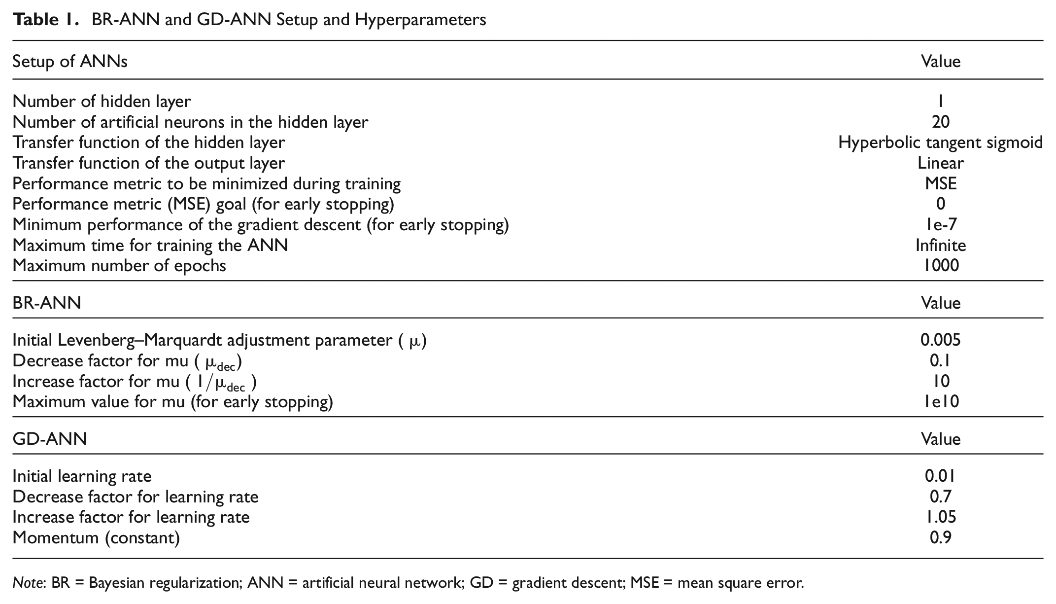
The calibration process may conclude in several ways. First, there is a fixed maximum number of epochs. In the present case, considering that the BR backpropagation algorithm is efficient in training ANNs (it does not require a high number of epochs for converging to a stable solution), the maximum number of epochs was fixed to 1000. Once trained, we can evaluate whether the specified number of epochs allows the BR-ANN to stabilize and, therefore, whether it is appropriate. The GD-ANN is trained across the same number of epochs.

Moreover, some “early stopping” criteria can stop the training process before reaching 1000 epochs. As for the BR-ANN, the training phase is interrupted if the chosen performance metric (i.e., the MSE) reaches zero, if the gradient becomes 10⁻⁷, and if the $μ$ value grows up to 10¹⁰. The GD-ANN training stops if the MSE reaches zero or the gradient becomes 10⁻⁷. The early stopping criteria should alleviate potential overfitting issues. Initial setup and additional hyperparameters concerning BR-ANN and GD-ANN calibration are recapped in Table 1.

Table 1.

BR-ANN and GD-ANN Setup and Hyperparameters

Setup of ANNs	Value
Number of hidden layer	1
Number of artificial neurons in the hidden layer	20
Transfer function of the hidden layer	Hyperbolic tangent sigmoid
Transfer function of the output layer	Linear
Performance metric to be minimized during training	MSE
Performance metric (MSE) goal (for early stopping)	0
Minimum performance of the gradient descent (for early stopping)	1e-7
Maximum time for training the ANN	Infinite
Maximum number of epochs	1000
BR-ANN	Value
Initial Levenberg–Marquardt adjustment parameter ( $μ$ )	0.005
Decrease factor for mu ( $μ_{dec}$ )	0.1
Increase factor for mu ( $1 / μ_{dec}$ )	10
Maximum value for mu (for early stopping)	1e10
GD-ANN	Value
Initial learning rate	0.01
Decrease factor for learning rate	0.7
Increase factor for learning rate	1.05
Momentum (constant)	0.9

Note: BR = Bayesian regularization; ANN = artificial neural network; GD = gradient descent; MSE = mean square error.

Readers may consider these values as starting parameters for setting up new ANNs or making comparisons with those already developed.

Once trained, the assessment phase of ANNs was performed by computing the R² (Equation 11) and RMSE (Equation 12):

R^{2} = 1 - \frac{\sum_{i = 1}^{N} {(\hat{Y_{i}} - Y_{i})}^{2}}{\sum_{i = 1}^{N} {(Y_{i} - \bar{Y_{i}})}^{2}}

(11)

RMSE = \sqrt{\frac{1}{N} {\sum_{i = 1}^{N} [(\hat{Y_{i}} - Y_{i})]}^{2}}

(12)

where $\hat{Y_{i}}$ is the predicted value of the target output for the $i$ th element, $Y_{i}$ is the observed value of the target output for the $i$ th element, $\bar{Y_{i}}$ is the averaged observed value of the target output $Y$ , and $N$ is the size of the set for which the $R^{2}$ is computed (training set, test set).

Furthermore, to numerically evaluate the capability of ANNs in avoiding overfitting issues, we computed the OR, defined as in Equation 13;

OR = \frac{RMS E_{test}}{RMS E_{train}}

(13)

where $RMS E_{test}$ is the $RMSE$ computed during the test phase and $RMS E_{train}$ is the $RMSE$ computed during the training phase. When the OR parameter is close to unity, this indicates a satisfactorily fitted model. On the other hand, an OR value of more than unity implies that a model may suffer from overfitting ( 25 ).

Moreover, we realized the scatterplot and residual distribution plots for both the training and test set as graphical performance metrics.

As a final assessment, it is possible to evaluate the importance of each input feature in predicting the target output. Therefore, the predictor importance (PI) is computed according to the procedure described in the works of Breiman ( 42 ), where a random forest algorithm is employed. Random forest is an ensemble learner incorporating several uncorrelated classification and regression tree (CART) single learners. The CART algorithm is a well-known tree-based learner with the task of identifying an appropriate tree structure that divides the training set into subgroups (called homogeneous nodes) through specific decision rules. The CART algorithm learns these rules automatically through the recursive partitioning algorithm, which identifies, starting from the first node of the tree (root node) to the final nodes (leaf nodes), the best decision rules for splitting data homogeneously. Predictors that are considered multiple times and those that are considered across the first levels of the CART have a high PI. Therefore, high PI corresponds to predictors that enable splitting the data set into homogeneous subgroups considering the target output; accordingly, these predictors should have a high correlation with the target output. Readers may find interesting the first study on the development of the CART algorithm made by Breiman et al. ( 43 ) and tutorials on how to compute PI ( 42 , 44 ).

Study Area and Data Collection

Study Area

The present research is focused on the Florence–Pisa–Leghorn (FPL) road, located in the Tuscany Region, central Italy (Figure 4). As the name suggests, that road connects three major cities in the region. The overall length of the FPL road is equal to 97 km and offers 30 well-distributed road interchanges. The FPL road is classified as a four-lane divided road; Italian standards ( 45 ) indicate for such facilities a minimum lane width of 3.75 m, minimum left shoulder width of 0.50 m, minimum right shoulder width of 1.75 m, a minimum planimetric radius of 178 m, a maximum longitudinal gradient of ±6%, and a maximum design speed of 120 km/h. Figure 4 shows the localization of the FPL road (red line), the urban centers (light blue polygons), the provinces crossed (Florence in green, Pisa in orange, and Leghorn in yellow), and the provinces not crossed in gray.

Figure 4.

Study area and Florence–Pisa–Leghorn (FPL) road investigated.

Data Collection and Input Features

The data was provided by the Tuscany Region Road Administration (TRRA). Specifically, TRRA provided information concerning geometrical aspects (horizontal and vertical alignment, road section geometry), functional aspects (traffic flows, operating speeds), and crash history records.

The present research considered the Florence–Pisa travel direction for an overall length of 78 km and 19 road interchanges. By exploiting a geographical information system (GIS) environment ( 46 ), 10 input features and 236 homogeneous road elements were defined. Such elements have a length that spans from 0.1 to 0.97 km. We chose 0.1 km as a minimum value for avoiding zero inflation issues. The maximum length was not constrained by a specific value. Within this range, the homogeneous road sections have unchanged geometric characteristics. For instance, the most extended section identified (i.e., a road segment with a length of 0.97 km) is a straight road section in which the width of the lanes, the left shoulder, the right shoulder, and so forth, do not change. The input features that were defined are as follows:

Length of the road element, L (km);

Planimetric curvature, C (1/m) (road segments have a planimetric curvature of zero);

Longitudinal gradient, G (%);

Lane width, LW (m);

Right shoulder width, RSW (m);

Left shoulder width, LSW (m);

Average annual daily traffic, AADT (vpd [vehicles per day]);

Operating speed, OS (km/h);

Sight distance, SD (m);

Road area type, A [accounting for the presence or absence of potential influence on the FPL road of merge and diverge influence areas of road interchanges].

Geometrical Predictors

TRRA provided road alignment in shapefile format. It is composed of straights, circular curves, and transition curves; for the present analysis, transition and circular curves are fitted with an interpolating circular curve. Therefore, we computed the radii of circular interpolated curves and the resulting planimetric curvature using a GIS environment. The curvature (predictor C), instead of the planimetric radius, allows associating a value with all the data set elements, also for the straights. Indeed, the straights are associated with a planimetric curvature value of zero (1/m).

Lane widths, left shoulder width, and right shoulder width were extracted from a data set of high-precision orthophotogrammetric images realized by TRRA in 2019. Such geometrical predictors were joined to the road alignment using spreadsheets and a GIS environment.

Finally, information on longitudinal gradient was provided by TRRA in spreadsheet format, reporting the location where longitudinal gradient changes and its value.

Traffic Flow

The AADT was detected yearly (from 2015 to 2019) through eight survey stations located on the analyzed road network. To be exploited as an input predictor in ANNs, the AADT values were averaged for each road segment. Furthermore, to evaluate how the traffic flow is distributed on the FPL road, we took advantage of a survey of 39 traffic stations positioned on the entry or exit ramps of road interchanges of the FPL road. In addition, a traffic assignment model with an origin–destination matrix was constructed in 2015 for all the roads of the Tuscany Region, allowing us to verify the actual traffic flow on the FPL road elements far from the survey stations.

Operating Speed

As evidenced by the input feature list, the operating speed was considered. Such a speed stems from actual speed measurements through radars. Indeed, a survey performed through seven stations equally distributed on the FPL road was available, from which the actual speeds of the vehicles were collected. First, the distribution of actual speeds was obtained for each station; subsequently, we considered the 85th percentile of the distribution as operating speed.

In the framework of this research, it is worth noting that the computation of operating speed, instead of the posted speed limit, is essential as the users are primarily habitual, using the FPL road for home–work commuting. Indeed, drivers select their speeds according to their perception of the road (i.e., operating or operational speed) rather than the designer’s perception (i.e., design speed) ( 47 ) or that imposed by the posted speed limit. In the present case study, the actual speed maintained by users is significantly higher than the posted speed limit, which is 90 km/h on the entire road. Therefore, posted speed limit would not have represented the actual behavior of users and would not have an appropriate association with the actual safety/criticality of road elements.

As an example, readers may observe Figure 5 showing the distribution of actual speed maintained by users where the posted speed limit equals 90 km/h (green dashed line). The resulting operating speed equals 127 km/h (blue dashed line).

Figure 5.

Distribution of actual speeds and computation of the operating speed (OS).

Sight Distance

The sight distance was derived geometrically through the definition of the FPL road in a computer aided design (CAD) environment once the road alignment and the longitudinal gradient were available. It is worth noting that the sight distance can be longer than the length of the associated homogeneous section, as a user can see beyond the end of the section. This happens, for example, in straights, when there is a change in the geometry of the cross section (lane width, left shoulder width, right shoulder width).

Road Area Type

As evidenced by the input feature list, road area type is a binary categorical predictor accounting for the presence (A = 1) or absence (A = 0) of potential influence on the FPL road caused by merge and diverge influence areas of road interchanges. According to the Highway Capacity Manual ( 48 ), it is worth mentioning that merge influence areas have a length of 450 m after the entry ramp (including the acceleration lane), while diverge influence areas have a length of 450 m before the exit ramp (including the deceleration lane). Therefore, traffic flows may be altered and suffer from turbulences if the associated road element lies within these areas. We identified 117 road elements with the absence of influence and 119 road segments with the presence of influence by merge or diverge influence areas of road interchanges.

Output Target

The output target to be predicted by the BR-ANN is the number of FI crashes that may occur in 5 years. TRRA provided the records of 3414 FI crashes that occurred across the whole FPL road between 2015 and 2019. It is worth mentioning that property-damage-only crashes are not included in the present data set since the Italian standards do not consider them for road safety analyses ( 49 ). Therefore, for the FPL road, TRRA was able to provide FI records only.

Descriptive Statistics

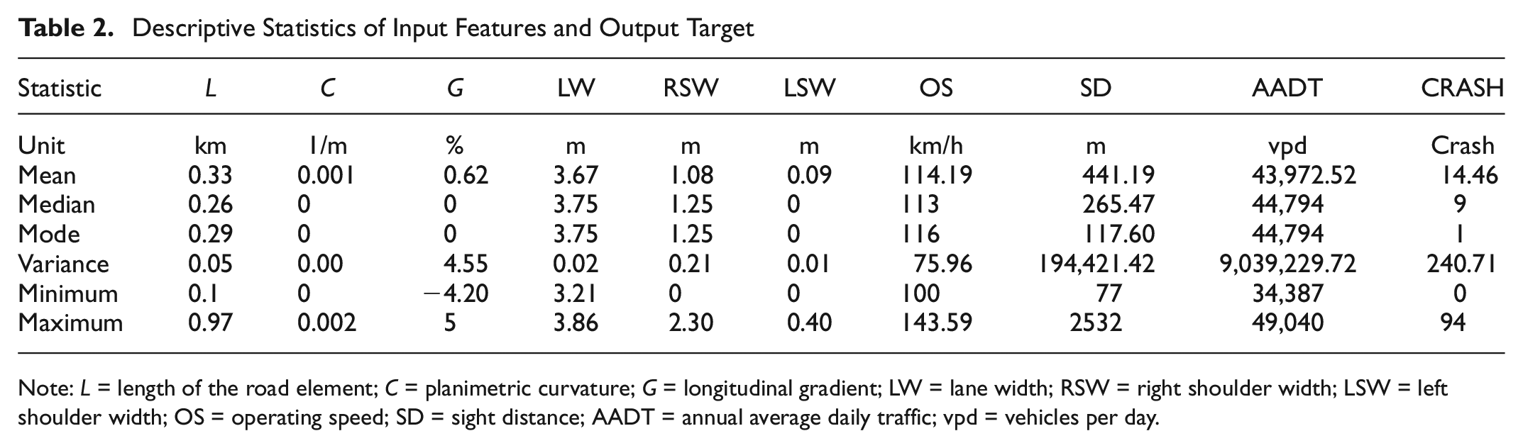
Table 2 reports the descriptive statistics of the numerical input features and output target. The definitions of input features and the output target have been reported in the above subsections.

Table 2.

Descriptive Statistics of Input Features and Output Target

Statistic	L	C	G	LW	RSW	LSW	OS	SD	AADT	CRASH
Unit	km	1/m	%	m	m	m	km/h	m	vpd	Crash
Mean	0.33	0.001	0.62	3.67	1.08	0.09	114.19	441.19	43,972.52	14.46
Median	0.26	0	0	3.75	1.25	0	113	265.47	44,794	9
Mode	0.29	0	0	3.75	1.25	0	116	117.60	44,794	1
Variance	0.05	0.00	4.55	0.02	0.21	0.01	75.96	194,421.42	9,039,229.72	240.71
Minimum	0.1	0	−4.20	3.21	0	0	100	77	34,387	0
Maximum	0.97	0.002	5	3.86	2.30	0.40	143.59	2532	49,040	94

Note: L = length of the road element; C = planimetric curvature; G = longitudinal gradient; LW = lane width; RSW = right shoulder width; LSW = left shoulder width; OS = operating speed; SD = sight distance; AADT = annual average daily traffic; vpd = vehicles per day.

The LW parameter manifests a lower average value (3.67 m) than the standard one (3.75 m), and a significantly lower minimum value (3.21 m). The RSW parameter reveals that there are road elements without a right paved shoulder (0.00 m) and an average value (1.08 m) significantly lower than the standard one (1.75 m). The same can be said for the LSW parameter: an average value equal to 0.09 m does not comply with Italian standards (0.50 m), and most of the road elements do not present a left paved shoulder (mode equal to 0.00 m). Observing the values of the mode, we can appreciate that the FPL road extends principally in straight sections (mode of C equal to 0.00 [1/m]), with zero G, and with OS higher (116 km/h) than the speed limit (90 km/h) in most of the road elements. The AADT does not report significant deviations across road elements, with a minimum of 34,387 vpd and a maximum of 49,040 vpd.

The target output is heavily over-dispersed (variance significantly higher than the mean). The minimum value is zero FI crashes (confirming the non-negativity of the CRASH parameter), and the mode value is 1 FI crash; consequently, there should be no zero inflation issues.

Results and Discussion

ANN Calibration

Figure 6 reports the MSE value during learning epochs of both BR-ANN (Figure 6a) and GD-ANN (Figure 6b).

Figure 6.

ANNs performance during epochs: (a) BR-ANN and (b) GD-ANN.

Figure 6 reports a substantial diversity in the performance during the training and test phases of the calibrated ANNs. Indeed, in Figure 6a, after an unstable behavior across 200 epochs, the BR-ANN tends to stabilize its performance horizontally during the training phase (blue line). Therefore, the BR-ANN cannot improve further, and 1000 learning epochs are enough to train the network. The test phase (red line in Figure 6a) shows that the performance is wholly coherent with the training one. This aspect confirms that overfitting issues are not present and that the BR-ANN can generalize appropriately on new data. It is worth mentioning that the $E_{s}$ parameter is equal to the MSE value at the end of the training phase (66.92). Conversely, as shown in Figure 6b, GD-ANN performance is not stable. It is clear that from about 100 epochs onwards, there is a substantial deviation between performance during training and performance during the test. Moreover, this gap grows more and more; at the end of the calibration cycle, the MSE for the training phase is equal to 49.78, whereas the MSE for the test phase is equal to 153.57. This dramatic reduction in performance is a clear symptom of the overfitting issue suffered by the GD-ANN. Accordingly, we expect that the GD-ANN cannot generalize properly on new data.

To evaluate the characteristic parameters of the ANNs, Figure 7 shows their values during the training process.

Figure 7.

Training process of ANNs: (a) BR-ANN and (b) GD-ANN.

After some preliminary adjustments (because of the initial random synaptic weights), the BR-ANN behavior highlighted in Figure 7a tends to stabilize, showing more regular trends during the epochs. After reaching 300 epochs, the characteristic parameters shown in Figure 7a (i.e., gradient, $γ$ , $μ$ ) assume a steady pattern. The BR-ANN has been regularized; as we can see in the last plot of Figure 7a, the $γ$ parameter is equal to 52.91 (i.e., 52.91 out of 241 network parameters are effectively used for decreasing the objective function to be minimized). Moreover, according to Equations 6 and 7, we computed an $α$ parameter of 1.23 and a $β$ parameter of 1.98 (the $E_{w}$ parameter is equal to 13.36). Considering that $β > α$ , as further confirmation, the BR learning process provided a significant size reduction of synaptic weights and the network does not suffer from overfitting issues.

As for the characteristic parameters of the GD-ANN (i.e., gradient and learning rate) highlighted in Figure 7b, we can see that an adaptive learning rate allows the gradient not to get stuck in certain local minima. Indeed, as soon as the gradient tends to no longer decrease significantly, the learning rate notably increases its value; this allows the gradient to continue to decrease over the epochs, searching for a global minimum. Furthermore, increases in learning rate are also reflected in the objective function of the GD-ANN; as shown in Figure 6b, there are oscillations of the MSE in conformity with the epochs in which the learning rate assumes maximum values.

ANN Assessment

To evaluate the performance of BR-ANN and GD-ANN, Figure 8 reports the scatterplot and the R² parameter of the training and test phases. Concerning the BR-ANN (Figure 8a), it can be appreciated that samples are adequately arranged on a line close to that of 45°, which indicates the perfect correlation between predictions and observations. No outliers or atypical clusters are present since there are neither points far away from the fitting line nor points concentrated in certain erroneous areas of the scatterplots. Predictions on road elements with low observed FI crashes (roughly between zero and 10 FI crashes) appear more accurate. This aspect reflects that most road elements have experienced a low number of FI crashes. By observing the parameter R², we can verify that the performances of the BR-ANN are both adequate and stable between the training phase (R² = 0.728) and the test phase (R² = 0.721). This aspect is additional proof that the BR-ANN does not suffer from overfitting issues, and it allows for making adequate predictions on new data. Indeed, there are no excessively deviated predictions in the test phase; the fitting line (red line) remains close to that of 45° with a slope comparable to the fitting line of the training phase (blue line).

Figure 8.

Scatterplot and R² parameter of ANNs: (a) BR-ANN in the training phase and test phase and (b) GD-ANN in the training phase and test phase.

In respect of the GD-ANN (Figure 8b), we can observe that the performances in the training phase are adequate (R² = 0.800), whereas a dramatic drop in performance occurs in the test phase; the R² parameter is less than half of that obtained in the training phase (R² = 0.359), highlighting that the GD-ANN suffers from severe overfitting issues. Consequently, we can confirm that the GD-ANN is unable to generalize on new data properly. Indeed, Figure 8b highlights that the points in the test scatterplot do not distribute according to a well-defined pattern and that the fitting line (red line) deviates substantially from the 45° line, confirming the above aspects.

The calculation of the RMSE provides information on the accuracy of predictions since this parameter corresponds to the standard deviation of the residual distribution. The RMSE of the BR-ANN is stable between the training and test phases, equal to 8.810 for the training phase and 7.503 for the test phase; this highlights that the BR-ANN does not suffer a reduction in performance. As for the GD-ANN, the RMSE of the test phase is significantly higher (12.392) than that obtained in the training phase (7.055), demonstrating a significant reduction in performance and a symptom of overfitting. This issue is particularly emphasized by computing the OR parameter. Indeed, the resulting OR for BR-ANN is 0.85 (i.e., close to the unity), while for the GD-ANN, OR is 1.76, thus showing a high tendency to overfit data.

The RMSE and OR are aggregate metrics helpful in making comparisons between different ANNs, but they cannot recognize how the error is distributed among the road elements. Plotting the residual distribution allows appreciating this aspect. Consequently, in Figure 9, residual distributions for both the BR-ANN (Figure 9a) and the GD-ANN (Figure 9b) are shown.

Figure 9.

Residuals distribution for ANNs: (a) BR-ANN and (b) GD-ANN.

Figure 9a shows that the residual distribution of the BR-ANN predictions is Gaussian and well centered in zero. The error is less than ±0.5 FI crashes on about 20% of road elements, while the error falls within the range [−3, +2] FI crashes on about 50% of road elements. Also, the distribution is not skewed; consequently, we can say that there is no range of values in which the BR-ANN overestimates or underestimates the FI crash count.

Figure 9b demonstrates that the residual distribution is similar to the previous one in shape but not in values; indeed, the distribution is Gaussian with zero mean, but the extreme values are higher (especially in the left tail of the distribution). The distribution is skewed, and most of the error lies in the positive values; consequently, GD-ANN tends to underestimate the value of FI crashes. We can recognize the overfitting since the distribution of residuals has a high kurtosis value, with few road elements associated with a significant error and many road elements with minimal error.

Once established that the BR-ANN is appropriate for accomplishing the present task, we deployed such a network for the FPL road. Therefore, we trained the BR-ANN with all available road elements. Figure 10 shows the resulting scatterplot and the R² parameter.

Figure 10.

Scatterplot and R parameter of BR-ANN at the deployment stage.

Figure 10 shows that the BR-ANN has a satisfying performance comparable to those outlined in Figure 8a. The synaptic weights are optimized for exploiting the BR-ANN on the whole FPL road. Nonetheless, they can be recalibrated for employing the network in different contexts. Even in this case, it is worth mentioning that the learning process continued for 1000 epochs and that the resulting RMSE is equal to 8.076.

Predictor Importance

As a final assessment, Figure 11 reports the PI value of each input feature. The definition and extended description of input features have been reported in the “Study Area and Data Collection” section.

Figure 11.

Predictor importance.

Figure 11 could provide road authorities with some information on where to focus in managing the FPL road by implementing specific design interventions. As previously specified, the computation of PI should allow the determination of the most influential conditioning factors for crash likelihood. Nonetheless, PI has to be judged qualitatively and not quantitatively since it is strictly related to the splitting process made by the random forest algorithm when growing CARTs. Indeed, it is worth underlining that a low PI value can also reflect the low variability of predictor values across road elements ( 42 ), and the algorithm perceives that such factors are not essential in crash likelihood. Unfortunately, this aspect is a limitation of data-driven models, which, operating as a “black box,” do not allow the analyst to obtain always defendable and accurate conclusions of the implication of predictors on the target output, especially with data sets of small sample size.

Road area type predictor (variable A) is categorical, and its high impact on crash likelihood should be evaluated differently from other numerical predictors. Indeed, being binary, predictor A divides the sample into two distinct subsamples. When the random forest algorithm grows a CART learner, predictor A is likely the first considered as the root node. Therefore, it assumes high importance since the CART ranks the predictor A first when deciding how to split the data set initially; this is presumably related to predictor A allowing splitting into two branch nodes with the highest degree of purity if compared with a splitting made by the other predictors. Therefore, in this case, it is not guaranteed that A has such high importance compared with the other predictors in determining crash likelihood since other road predictors have low variability across road elements, while A markedly divides the data set into two subsamples.

Furthermore, from Figure 11, it can be deemed that the length of road sections (variable L) assumes high importance. Once again, we may presume that such a high value is observed since significantly different accident levels are recorded between short sections (with zero or very few accidents) to long sections (generally, many accidents are recorded). Therefore, the random forest algorithm perceives that the length of a road section is an essential element in predicting crash likelihood when, in general, predictor L is a scale parameter of the accident count observed in a section.

Considering the geometrical predictors, Figure 11 emphasizes that the right shoulder width (variable RSW) is the most important. Considering that the variability of predictors C, G, LW, LSW, and RSW across road elements is similar, we can deem that RSW is the most important geometrical parameter in determining the number of accidents that may occur among those considered. An adequate right shoulder width allows vehicles to anticipate obstacles around a curve and allows for early observation of lay-bys, which are quite common on the FPL road. Moreover, the RSW probably has a significant relationship with the FI crash likelihood since in road elements where RSW is low (i.e., lower than the standard value of 1.75 m), the vehicles tend to move at the center of the carriageway, limiting the overtaking lane, constituting a risk of sideswipe collisions, thus increasing the number of crashes that may occur. This phenomenon occurs mainly at curves since users attempt to increase their limited sight distance. Such a correlation between RSW and sight distance (variable SD) may reflect the substantial importance of both predictors and operating speed (variable OS); indeed, generally, high values of SD are related to high values of OS. It is conceivable that users tend to select high speeds with a high SD available.

Finally, Figure 11 shows the relatively low importance of the traffic flow (variable AADT); albeit counterintuitive, as previously specified, the low importance likely reflects the low variability of AADT values across road elements.

Finally, as an additional evaluation phase, we carried out an in situ survey to assess the leading criticalities related to the effect on the FPL road of merge and diverge influence areas. Therefore, we focused on analyzing road interchanges connecting the secondary road network (generally composed of two-lane rural and urban roads) to the FPL road. From the survey, the following points emerged.

Most of the entry ramps do not have sufficient acceleration lane length; consequently, entry vehicles force those on the FPL road to brake abruptly or to move into the overtaking lane, creating significant turbulence in the traffic flow and potential rear-end and sideswipe collisions.

Most exit ramps must be crossed at a slower speed than the posted one for the FPL road (90 km/h) since the planimetric radii of the exit ramps are often not compliant with current standards. Moreover, vehicles arrive on the exit ramps with an operating speed significantly higher than the posted speed limit, with potential risks of run-off accidents. Indeed, exit ramps should be crossed with a speed of about 40 km/h (according to planimetric radii of exit ramps of 40–45 m). This aspect is related to the investigated Florence–Pisa road stretch being built between the 1970s and the 1990s; most of the road interchanges have been designed according to previous standards, considering a significantly lower value of traffic flow and users’ speed.

Lengths of the deceleration lanes of most exit ramps are not adequate; consequently, vehicles tend to start the braking phase on the FPL road, with the potential risk of rear-end collisions.

There are areas in which entry ramps preceding exit ramps are close together; accordingly, critical, ill-designed weaving segments arise, causing potential FI crashes.

There are road segments where lay-bys or service areas interfere in the merge or diverge influence areas. Consequently, criticalities arise between the vehicles that want to enter or exit the FPL road and those who stop in or leave these parking areas. As a result, the turbulences in traffic flow markedly increase, and the operating speed decreases, thus reducing traffic quality (level of service) and lowering the safety level of the FPL road.

Future Work

The proposed methodology has highlighted both the strengths of BR-ANNs in predicting FI crash occurrences across Italian four-lane divided roads and some weaknesses. To improve the present research, these could be considered as starting points for future works.

First, considering that the sample size is small and that the performance of predictive models (both parametric and nonparametric) markedly depends on the contours of training and testing data, the use of synthetic data may be helpful for artificially increasing the sample size, thus training models with appropriate train/test samples.

Moreover, it could be beneficial to know whether the benefits of BR-ANN are attributed to the regularization term, the Bayesian method, or both. Therefore, to propose a more objective comparison between ANNs, we may include a regularization term (i.e., a weight decay) into the loss function of the GD-ANN.

Furthermore, as previously specified, the output of BR-ANN can be sensitive to the choice of the prior probability of weights. As a common practice, in the present research, we used a Gaussian prior distribution. Therefore, additional prior distributions, such as Laplace or double exponential, could be of particular novelty and interest to the academic community.

Finally, it could be interesting to compare the present BR-ANN performance with that of statistical count models. Indeed, we could calibrate a local safety performance function for the FPL road, for example by assuming a negative binomial distribution for fitting crash data, and evaluate whether count models are appropriate. Furthermore, if such models appropriately predict FI crashes, we may also quantify the impact of predictors on crash likelihood by computing marginal effects or elasticities. Accordingly, it should be possible to know precisely the effect of geometrical and functional characteristics on FI crash likelihood.

Conclusions

In the present paper, we aimed to emphasize the strengths of ANNs trained by the BR backpropagation algorithm in APMs, extending their implementation to four-lane divided roads, where no studies have been recognized. For this purpose, we calibrated an APM for FI crash prediction on Italian four-lane divided roads. With the need to handle a small sample size for the accident analysis, we have verified that an ANN trained by the BR backpropagation algorithm can efficiently alleviate overfitting issues and provide reliable predictions on new data. Indeed, by automatically pruning several synaptic weights, the algorithm allows for regularizing the learning process. Exploiting some performance metrics, namely determination coefficient, RMSE, scatterplots, and residual distribution plot, we proved that such an algorithm works properly; indeed, its performance between the training and test phases does not significantly decrease. Furthermore, in just over 300 epochs (i.e., a few seconds of training time), the characteristic parameters of the Bayesian regularized ANN, namely the Levenberg–Marquardt damping factor, the effective number of parameters, and the gradient, tend to stabilize and exhibit a horizontal pattern, highlighting that additional epochs are not required. Subsequently, as a comparing benchmark, we trained an ANN with the same architecture by the GD with momentum and adaptive learning rate backpropagation algorithm. We have verified that the latter suffers from serious overfitting issues and cannot make reliable predictions on new data. Indeed, during 1000 epochs of training, its performance between the training and test phase dramatically reduced. Therefore, this research supports the Bayesian regularized ANN as a promising algorithm in developing APMs, especially when small sample sizes are available.

Footnotes

Author Contributions

The authors confirm contribution to the paper as follows: study conception and design: N. Fiorentini, D. Pellegrini., M. Losa; data collection: N. Fiorentini, D. Pellegrini, M. Losa; analysis and interpretation of results: N. Fiorentini., D. Pellegrini, M. Losa; draft manuscript preparation: N. Fiorentini, D. Pellegrini, M. Losa. All authors reviewed the results and approved the final version of the manuscript.

Declaration of Conflicting Interests

The author(s) declared no potential conflicts of interest with respect to the research, authorship, and/or publication of this article.

Funding

The author(s) disclosed receipt of the following financial support for the research, authorship, and/or publication of this article: This work was supported by the Tuscany Region CMRSS (Regional Road Safety Monitoring Center) project promoted by the Tuscany Region as partial fulfillment of the aims of the National Plan of Road Safety (PNSS), funded by the Ministry of Infrastructure and Sustainable Mobility, Italy.

ORCID iDs

Nicholas Fiorentini

Diletta Pellegrini

Massimo Losa

References

World Health Organization. Global Status Report on Road Safety: Summary 2018. World Health Organization, Geneva, 2018.

Fiorentini

Losa

Handling Imbalanced Data in Road Crash Severity Prediction by Machine Learning Algorithms. Infrastructures, Vol. 5, No. 7, 2020, P. 61. https://doi.org/10.3390/infrastructures5070061.

Iranitalab

Khattak

Comparison of Four Statistical and Machine Learning Methods for Crash Severity Prediction. Accident Analysis & Prevention, Vol. 108, 2017, pp. 27–36. https://doi.org/10.1016/J.AAP.2017.08.008.

Rahim

M. A.

Hassan

H. M.

A Deep Learning Based Traffic Crash Severity Prediction Framework. Accident Analysis Prevention, Vol. 154, 2021, P. 106090. https://doi.org/10.1016/j.aap.2021.106090.

Theofilatos

Chen

Antoniou

Comparing Machine Learning and Deep Learning Methods for Real-Time Crash Prediction. Transportation Research Record: Journal of the Transportation Research Board, 2019. 2673: 169–178.

Hossain

Muromachi

A Bayesian Network Based Framework for Real-Time Crash Prediction on the Basic Freeway Segments of Urban Expressways. Accident Analysis & Prevention, Vol. 45, 2012, pp. 373–381. https://doi.org/10.1016/j.aap.2011.08.004.

Fiorentini

Losa

Long-Term-Based Road Blackspot Screening Procedures by Machine Learning Algorithms. Sustainability, Vol. 12, No. 15, 2020, P. 5972. https://doi.org/10.3390/su12155972.

Washington

Haque

M. M.

Lee

Applying Quantile Regression for Modeling Equivalent Property Damage Only Crashes to Identify Accident Blackspots. Accident Analysis & Prevention, Vol. 66, 2014, pp. 136–146. https://doi.org/10.1016/j.aap.2014.01.007.

Fiorentini

Leandri

Losa

Defining Machine Learning Algorithms as Accident Prediction Models for Italian Two-Lane Rural, Suburban, and Urban Roads. International Journal of Injury Control and Safety Promotion, 2022, pp. 1–13. https://doi.org/10.1080/17457300.2022.2075397

10.

Hall

Tarko

A. P.

Adequacy of Negative Binomial Models for Managing Safety on Rural Local Roads. Accident Analysis & Prevention, Vol. 128, 2019, pp. 148–158. https://doi.org/10.1016/j.aap.2019.03.001.

11.

Tang

Donnell

E. T.

Application of a Model-Based Recursive Partitioning Algorithm to Predict Crash Frequency. Accident Analysis & Prevention, Vol. 132, 2019, P. 105274. https://doi.org/10.1016/j.aap.2019.105274.

12.

Mannering

F. L.

Bhat

C. R.

Analytic Methods in Accident Research: Methodological Frontier and Future Directions. Analytic Methods in Accident Research, Vol. 1, 2014, pp. 1–22. https://doi.org/10.1016/j.amar.2013.09.001.

13.

Mannering

Bhat

C. R.

Shankar

Abdel-Aty

Big Data, Traditional Data and the Tradeoffs between Prediction and Causality in Highway-Safety Analysis. Analytic Methods in Accident Research, Vol. 25, 2020, P. 100113. https://doi.org/10.1016/j.amar.2020.100113.

14.

Yannis

Dragomanovits

Laiou

La Torre

Domenichini

Richter

Ruhl

Graham

Karathodorou

Road Traffic Accident Prediction Modelling: A Literature Review. Proceedings of the Institution of Civil Engineers: Transport, Vol. 170, No. 5, 2017, pp. 245–254. https://doi.org/10.1680/jtran.16.00067.

15.

Wang

Zhao

Jackson

Functional Forms of the Negative Binomial Models in Safety Performance Functions for Rural Two-Lane Intersections. Accident Analysis & Prevention, Vol. 124, 2019, pp. 193–201. https://doi.org/10.1016/j.aap.2019.01.015.

16.

Washington

S. P.

Karlaftis

M. G.

Mannering

F. L.

Anastasopoulos

. . Statistical and Econometric Methods for Transportation Data Analysis, 3rd ed. Chapman & HALL/CRC, New York, NY, 2020.

17.

Zhang

Comparing Prediction Performance for Crash Injury Severity among Various Machine Learning and Statistical Methods. IEEE Access, Vol. 6, 2018, pp. 60079–60087. https://doi.org/10.1109/ACCESS.2018.2874979.

18.

Alkheder

Taamneh

Severity Prediction of Traffic Accident Using an Artificial Neural Network. Journal of Forecasting, Vol. 36, No. 1, 2017, pp. 100–108. https://doi.org/10.1002/for.2425.

19.

Singh

Pal

Yadav

Singla

Deep Neural Network-Based Predictive Modeling of Road Accidents. Neural Computing and Applications, Vol. 32, No. 16, 2020, pp. 12417–12426. https://doi.org/10.1007/s00521-019-04695-8.

20.

Abdel-Aty

Haleem

Analyzing Angle Crashes at Unsignalized Intersections Using Machine Learning Techniques. Accident Analysis & Prevention, Vol. 43, No. 1, 2011, pp. 461–470. https://doi.org/10.1016/J.AAP.2010.10.002.

21.

Dong

Shao

Xiong

An Improved Deep Learning Model for Traffic Crash Prediction. Journal of Advanced Transportation, Vol. 2018, 2018, pp. 1–13. https://doi.org/10.1155/2018/3869106.

22.

Cawley

G. C.

Talbot

N. L. C.

Preventing Over-Fitting during Model Selection via Bayesian Regularisation of the Hyper-Parameters. Journal of Machine Learning Research, Vol. 8, 2007, pp. 841–861.

23.

MacKay

D. J. C.

Bayesian Interpolation. Neural Computation, Vol. 4, No. 3, 1992, pp. 415–447. https://doi.org/10.1162/neco.1992.4.3.415.

24.

Schlögl

Stütz

Laaha

Melcher

A Comparison of Statistical Learning Methods for Deriving Determining Factors of Accident Occurrence from an Imbalanced High Resolution Dataset. Accident Analysis & Prevention, Vol. 127, 2019, pp. 134–149. https://doi.org/10.1016/J.AAP.2019.02.008.

25.

Chakraborty

Mukherjee

Mitra

Development of Pedestrian Crash Prediction Model for a Developing Country Using Artificial Neural Network. International Journal of Injury Control and Safety Promotion, Vol. 26, No. 3, 2019, pp. 283–293. https://doi.org/10.1080/17457300.2019.1627463.

26.

Xie

Lord

Zhang

Predicting Motor Vehicle Collisions Using Bayesian Neural Network Models: An Empirical Analysis. Accident Analysis & Prevention, Vol. 39, No. 5, 2007, pp. 922–933. https://doi.org/10.1016/j.aap.2006.12.014.

27.

Riviere

Lauret

Ramsamy

J. F. F. M.

Page

A Bayesian Neural Network Approach to Estimating the Energy Equivalent Speed. Accident Analysis & Prevention, Vol. 38, No. 2, 2006, pp. 248–259. https://doi.org/10.1016/j.aap.2005.08.008.

28.

Mcculloch

W. S.

Pitts

A Logical Calculus of the Ideas Immanent in Nervous Activity. Bulletin of Mathematical Biophysics, Vol. 5, 1943, pp. 115–133. https://doi.org/10.1007/978-3-030-01370-7_61.

29.

Rumelhart

D. E.

Hinton

G. E.

Williams

R. J.

Learning Representations by Back-Propagating Errors. Nature, Vol. 323, No. 6088, 1986, pp. 533–536. https://doi.org/10.1038/323533a0.

30.

Lau

K. T.

Guo

Kiernan

Slater

Diamond

Non-Linear Carbon Dioxide Determination Using Infrared Gas Sensors and Neural Networks with Bayesian Regularization. Sensors and Actuators, B: Chemical, Vol. 136, No. 1, 2009, pp. 242–247. https://doi.org/10.1016/j.snb.2008.11.030.

31.

Yue

Songzheng

Tianshi

Bayesian Regularization BP Neural Network Model for Predicting Oil-Gas Drilling Cost. Proc., International Conference on Business Management and Electronic Information, IEEE, New York, 2011, pp. 483–487.

32.

Kayri

. Predictive Abilities of Bayesian Regularization and Levenberg-Marquardt Algorithms in Artificial Neural Networks: A Comparative Empirical Study on Social Data. Mathematical and Computational Applications, Vol. 21, No. 2, 2016, P. 20. https://doi.org/10.3390/mca21020020.

33.

Liang

An Effective Bayesian Neural Network Classifier with a Comparison Study to Support Vector Machine. Neural Computation, Vol. 15, No. 8, 2003, pp. 1959–1989. https://doi.org/10.1162/08997660360675107.

34.

Liang

Bayesian Neural Networks for Nonlinear Time Series Forecasting. Statistics and Computing, Vol. 15, No. 1, 2005, pp. 13–29. https://doi.org/10.1007/s11222-005-4786-8.

35.

Jaynes

E. T.

Prior Probabilities. IEEE Transactions on Systems Science and Cybernetics, Vol. 4, No. 3, 1968, pp. 227–241. https://doi.org/10.1109/TSSC.1968.300117.

36.

Foresee

F. D.

Hagan

M. T.

Gauss-Newton Approximation to Bayesian Learning. Proc., International Conference on Neural Networks (ICNN’97), Vol. 3, Houston, TX, IEEE, New York, 1997, pp. 1930–1935.

37.

Levenberg

Arsenal

A Method for the Solution of Certain Non-Linear Problems in Least Squares. Quarterly of Applied Mathematics, Vol. 1, No. 278, 1943, pp. 536–538.

38.

Marquardt

D. W.

An Algorithm for Least-Squares Estimation of Nonlinear. Journal of the Society for Industrial and Applied Mathematics, Vol. 11, No. 2, 1963, pp. 431–441.

39.

Fiorentini

Leandri

Losa

Predicting International Roughness Index by Deep Neural Networks with Levenberg-Marquardt Backpropagation Learning Algorithm. Proc., SPIE 11863, Earth Resources and Environmental Remote Sensing/GIS Applications XII, Vol. 11863, 118630P, September12, 2021, pp. 194–207. https://doi.org/10.1117/12.2598005.

40.

Géron

Hands-on Machine Learning with Scikit-Learn, Keras, and TensorFlow: Concepts, Tools, and Techniques to Build Intelligent Systems. O’Reilly Media, Sebastopol, CA, 2019.

41.

Kohavi

A Study of Cross-Validation and Bootstrap for Accuracy Estimation and Model Selection. Proc., 14th International Joint Conference on Artificial Intelligence, American Association for Artificial Intelligence, Montreal, Quebec, Canada, August 20–25, 1995, pp. 1137–1143.

42.

Breiman

Random Forest. Machine Learning, Vol. 1, 2001, P. 33. https://doi.org/10.1023/A:1010933404324.

43.

Breiman

Friedman

J. H.

Olshen

R. A.

Stone

C. J.

Classification and Regression Trees. Chapman & Hall/CRC, New York, 1984.

44.

Louppe

Wehenkel

Sutera

Geurts

Understanding Variable Importances in Forests of Randomized Trees. Advances in Neural Information Processing Systems, Vol. 26, 2013, pp. 1–9.

45.

Ministry of Infrastructure and Transport. Decreto Ministeriale 5 Novembre2001, n. 6792 (S.O. n.5 Alla G.U. n.3. Del 4.1.02) Norme Funzionali e Geometriche per La Costruzione Delle Strade.

46.

ESRI. ArcGIS Desktop: Release 10.5. Environmental Systems Research Institute, Redlands, CA, 2011.

47.

Misaghi

Hassan

Modeling Operating Speed and Speed Differential on Two-Lane Rural Roads. Journal of Transportation Engineering, Vol. 131, No. 6, 2005, pp. 408–418. https://doi.org/10.1061/(ASCE)0733-947X(2005)131:6(408).

48.

National Research Council of the Transportation Research Board. Highway Capacity Manual 6th Edition: A Guide for Multimodal Mobility Analysis. Transportation Research Board, Washington, DC, 2016.

49.

Ministry of Infrastructure and Transport. Decreto Ministeriale Numero 137 Del 02/05/2012, Linee Guida per La Gestione Della Sicurezza Delle Infrastrutture Stradali Ai Sensi Dell’art. 8 Del Decreto Legislativo 15 Marzo 2011, n. 35.