
Abstract
The main goal of the current study is to identify the factors affecting flight-level airline delay by jointly modeling departure and arrival delays. Toward this end, we develop a novel copula-based group generalized ordered logit (GGOL) model system that accommodates for the influence of common observed and unobserved effects on flight departure and arrival delays. The proposed model is estimated using 2019 marketing carrier on-time performance data compiled by the Bureau of Transportation Statistics (BTS) for 67 airports in the continental U.S. The delay data is augmented with a comprehensive set of independent variables including traffic conditions at the origin and destination airports in the hours preceding flight departure and arrival, trip-level attributes, weather variables for the entire flight duration, and spatial and temporal factors. The model estimation results highlight that the Joe copula model with parameterization provides the best data fit. The model performance is further established to be excellent using a holdout sample. Finally, to illustrate the applicability of the model for prediction and highlight the impact of independent variables, we perform a prediction exercise under a host of hypothetical scenarios. The illustration provides a mechanism for employing the proposed model as a tool for airline-carrier-level or airport-level delay prediction analysis using weather forecasts while controlling for a host of independent variables.
Keywords
In the United States, the domestic airline industry is a key contributor to the economy. According to the Federal Aviation Administration (FAA), the commercial aviation industry accounts for 5.2% of U.S. Gross Domestic Product ( 1 ). According to the Bureau of Transportation Statistics (BTS), 19.79% of all flights operated in the U.S. arrived late by 15 min or more in 2019 ( 2 ) (the highest such percentage since 2015). Airline delays cause both direct and indirect costs to several components of the industry. The cost of airline delays to passengers is estimated at $18.1 billion for 2019 ( 3 ). Costs to airlines from additional expenses for crews, fuel, and maintenance are estimated at $8.3 billion ( 3 ) not considering the impact of the worsening customer experience on airline attractiveness ( 4 ). Airline delays also cause indirect costs to different business sectors amounting to nearly $4.2 billion ( 3 ). Given these substantial negative impacts of airline delays on the U.S. economy, understanding the factors influencing airline on-time performance will allow airlines to improve their on-time performance or mitigate the delays by increasing and reallocating their resources such as aircrafts, crews, and staff.
In airline literature, airline delay can be considered as a departure or an arrival delay, or both. According to BTS, departure/arrival delay can be defined as the time difference between scheduled and actual gate departure/arrival time. Traditionally, earlier studies identified the factors affecting airline delays and developed prediction models. A summary of previous studies examining airline delay is provided in Table 1 with information on the delay measure of interest, spatial resolution of analysis, number of airports considered, study objectives, methodology employed, and independent variables considered. From Table 1, we can make several observations. First, earlier studies on airline delay consider three types of delay measures: (a) departure delay, (b) arrival delay, and (c) both departure and arrival delay. From the review, a majority of earlier research analyzed either departure or arrival delay. The studies, modeling both departure and arrival delays, modeled the two delay categories independently. Second, earlier research on airline delay is conducted at three resolutions: (a) flight, (b) airport, and (c) national airspace system (NAS) level. At the first resolution, studies analyze airline delay for individual flights while in the latter two resolutions, delay is analyzed at an aggregate level of airport or network as an average daily delay. The review also shows that earlier studies analyzed airline delay data mostly employing a limited set of airports. The 35 Operational Evolution Partnership airports (OEP-35) make up the largest set of airports considered by the airport-level studies ( 5 , 6 ). However, flight-level studies considered flights operated at most of the major airports across the U.S. Third, the factors considered in modeling airline delays vary across the studies and include traffic conditions (average queuing delay, average arrival delay, total operations), trip-specific factors (carrier, route, distance), weather conditions (visibility, wind speed, thunderstorm, precipitation, snow depth), spatial factors (location of origin and destination airports), and temporal factors (season, weekday/weekend, time of the day). Based on our review, weather factors considered in earlier research efforts can be grouped into three categories: airport level, route level, and NAS level. Some of these studies conducted comprehensive analysis to examine the effect of convective weather condition on flight delay. For example, Hsiao and Hansen ( 7 ) analyzed airline delay at the system level and considered airport-level and route-level weather conditions using grid variables. Yu et al. ( 8 ) also considered route-level weather conditions in a flight-level model and considered delay records of previous flights along the same route as a surrogate measure. Dai et al. ( 9 ) proposed a model system to determine NAS-level delay and employed system- and airport-specific weather variables in the model. Liu et al. ( 10 ) proposed an innovative approach to identify whether or not a flight may encounter a convective weather condition along its route, using multiple weather data sources. Fourth, several mathematical models were employed in the literature to predict airline delays and they can be broadly classified as (a) discrete outcome and (b) continuous outcome models. In discrete outcome models, the dependent variable is characterized as a binary outcome (flight delayed or not based on the BTS threshold of 15 min) or a categorical variable (for example, Gui et al. [ 11 ] categorized flight arrival delay in four groups). Among discrete outcome models, binary/multinomial logit models are generally employed to determine the factors affecting airline delay. Among continuous outcome models, where delay is measured in minutes, commonly employed models include (a) linear regression models, (b) time series analysis, (c) machine learning approaches, (d) survival models, (e) piecewise regression models, and (f) optimization methods. Finally, discrete outcome models are more commonly employed in flight-level analysis while continuous outcome models are employed in both disaggregate- and aggregate-level analysis.
Summary of Literature Review
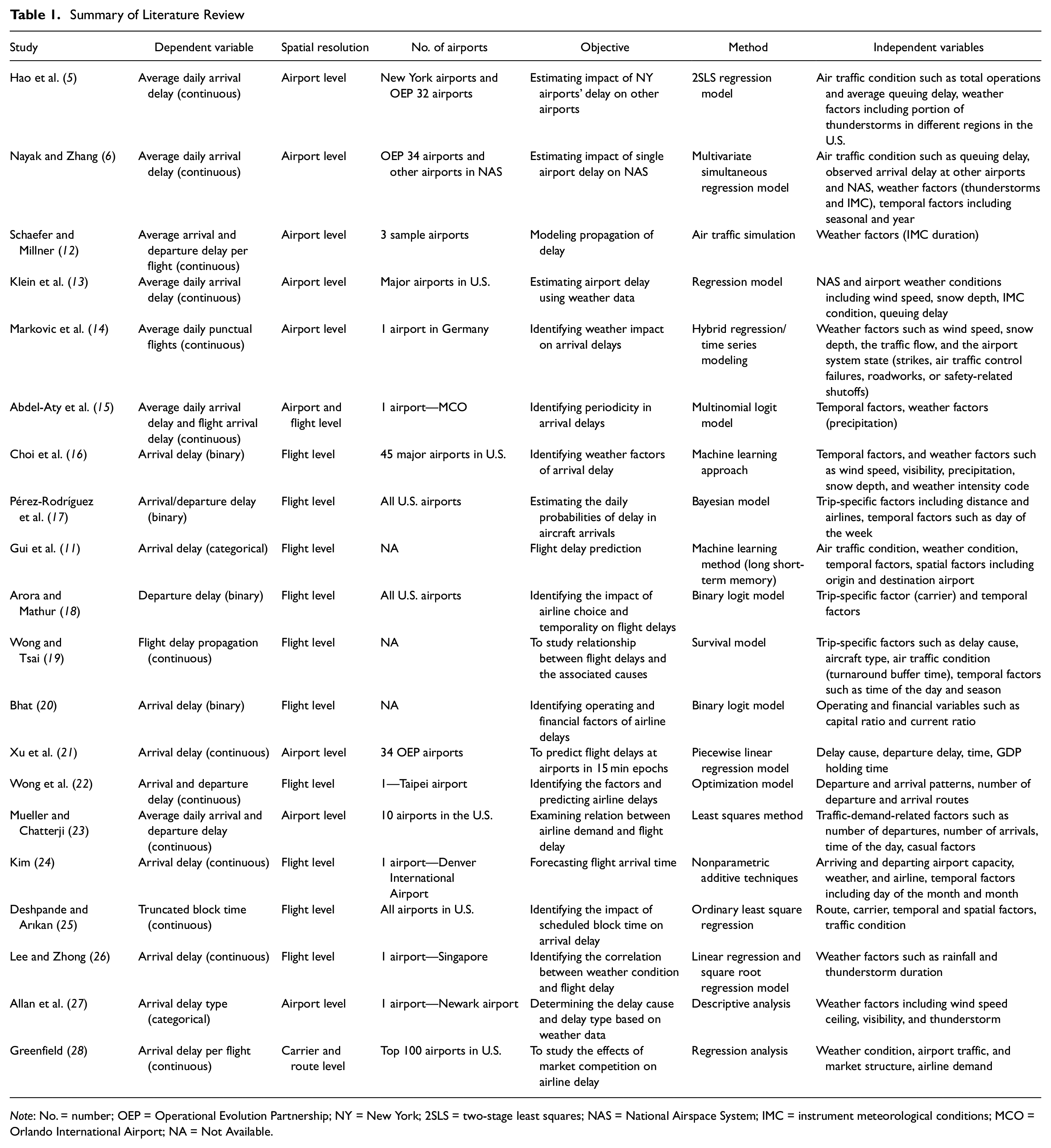
Note: No. = number; OEP = Operational Evolution Partnership; NY = New York; 2SLS = two-stage least squares; NAS = National Airspace System; IMC = instrument meteorological conditions; MCO = Orlando International Airport; NA = Not Available.
Contributions of the Current Study
In this study, our goal is to model departure and arrival delays in a joint framework at the disaggregate resolution of flights.
A major contribution of this study to literature arises from data enhancement for flight delay analysis. The variables processed from 2019 BTS marketing carrier on-time performance data are augmented with a comprehensive set of independent variables sourced from secondary data sources including the Automated Surface Observing System (ASOS) data set (sourced from Iowa Environment Mesonet) and FAA’s Aviation System Performance Metrics (ASPM). We prepare weather variables—wind speed, hourly precipitation, thunderstorm proportion, and visibility—from the ASOS data set. The data compilation is achieved by charting the potential airline flight route to identify weather conditions near the flight’s origin airport, along the route, and at the destination airport. Toward processing this weather data, we divide the continental U.S. into a latitude–longitude grid of 5 degrees and compile hourly weather data from all weather stations within each grid while estimating the flight path and its intersection with the grid system (more details in the Data Set Description section). The detailed process allows us to generate weather conditions for the entire duration of the flight. Subsequently, we employ ASPM data to determine air traffic conditions at the origin and destination airports in the hours preceding the flight’s departure and arrival, respectively. Finally, we perform spatial data enhancement in our study by considering all flights between 67 airports across the U.S. to capture the effects of spatial factors on flight-level delay. The selected 67 airports are a subset of ASPM 77 airports and include all OEP-35 airports in the U.S. The data for our analysis is augmented with other independent variables including (a) trip-specific factors (carrier and flight distance), (b) spatial factors (region of origin and destination airports), and (c) temporal factors (season, day of the week, and time of the day). The reader should note that the current study is the first effort to consider the influence on flight delay of high-resolution spatiotemporal weather conditions along the entire flight.
Employing the data prepared, the current research contributes to airport departure and arrival delay analysis by developing a novel copula-based group generalized ordered logit (GGOL) model. The proposed framework recognizes that a delay measure in minutes is not exclusively a categorical variable or a continuous variable. A cursory examination of the delay variable will indicate the presence of clusters of data points as delay increases: that is, as delay increases, it is likely to be rounded to larger time bins (such as 5 min or 15 min). For analyzing such data, the application of a purely discrete outcome model system, while feasible, does not allow the estimation of a continuous measure in prediction (without any strong assumptions). On the other hand, employing a continuous variable representation is not appropriate with rounded values. Thus, in our proposed research we employ a hybrid framework that ties the continuous delay measure to a categorical variable allowing us to estimate the model as a discrete outcome system with the inherent ability to predict as a continuous variable ( 29 – 31 ) (more details in the Econometric Methodology section).
Our proposed model system also recognizes that it is very plausible that there might be some common unobserved factors influencing both delay categories. Given the obvious interactions between the two types of delay variables, we develop a copula-based GGOL model framework that accommodates for the influence of common observed and unobserved effects on flight departure and arrival delays. In this study, we also estimate and parameterize the error variance of the delay component to account for heteroscedasticity. The two GGOL model components are then stitched together as a joint distribution using the flexible copula-based approach. In our analysis, we employ six different copula structures—the Gaussian copula, the Farlie–Gumbel–Morgenstern (FGM) copula, and a set of Archimedean copulas including Frank, Clayton, Joe, and Gumbel copulas (see Bhat and Eluru [ 32 ] for a detailed discussion). The value of the proposed model system is illustrated by comparing predictive performance of the proposed model relative to independent models of flight departure and arrival on a holdout sample (records not used in estimation). Finally, we conduct an application analysis to present the policy implications of the current research. The illustration provides a mechanism for employing the proposed model as a tool for airline-carrier-level or airport-level delay prediction analysis using weather forecasts.
The rest of the paper is divided into five sections. In the subsequent section, we present the econometric methodology employed in the research including the GGOL model and the bivariate copula model of departure and arrival delays. Next, we present data assembly and compilation procedures, and sample descriptive statistics in the Data Set Description section. The Analysis and Results section describes model selection processes, model estimation results, and the validation exercise. The Model Illustration section presents the application of the proposed model using different hypothetical scenarios of origin, route, and destination weather conditions. Finally, the concluding remarks are included in the last section.
Econometric Methodology
In this section, econometric formulation of the copula-based GGOL model is presented. First, we present the formulation of independent GGOL models of flight departure and arrival delay. In independent GGOL models, we estimate two separate model systems without any dependency between the dependent variables. In the bivariate copula model, we consider the dependency between the departure and arrival delays by using different copula dependency profiles.
Flight Delay Model
Let q (q = 1,2,…,Q), and k (k = 1,2,…,K; K = 2) be the indices to represent flight and the corresponding delay type (departure/arrival), respectively. Let
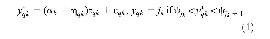
where

where
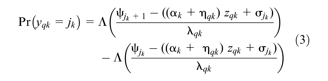
where
Bivariate Copula Model
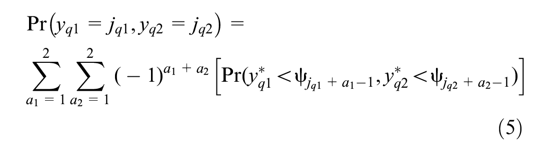
In examining the grouped time intervals across two delay types simultaneously, the levels of correlations between two dimensions of interests depend on the type and extent of dependency among the stochastic terms
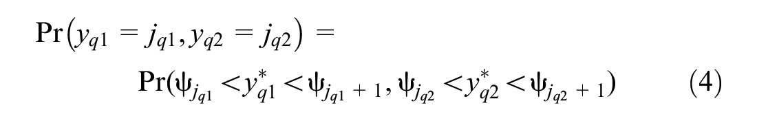
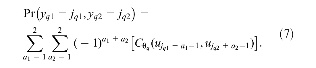
Now, Equation 4 can be written as follows ( 33 ):
The copula is a device or function that generates a stochastic dependence relationship (i.e., a multivariate distribution) among random variables with prespecified marginal distributions ( 32 ), and can be defined as
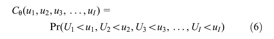
where
To allow for the dependency structure to vary across flights, the dependence parameter

where
In examining the model structure of flight delay across two delay types, it is also necessary to specify the structure for the unobserved vector
where

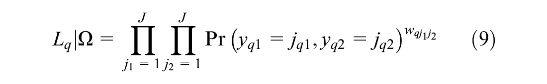
Now, we can express the log-likelihood function as follows:

The parameters to be estimated in the copula model are
Data Set Description
The main data for our study is drawn from the BTS 2019 non-stop domestic marketing carrier on-time performance data set. The marketing on-time performance data set includes departure and arrival data for 10 marketing carriers who market flights for themselves and their regional code share partners. The on-time performance data set offers flight-level information including scheduled and actual gate departure/arrival date and time, departure/arrival delay in minutes, delay cause, cancellation and diversion indicator, origin and destination airports, marketing carrier, and operating carrier. Initially, we started our analysis considering all the 77 ASPM airports. However, 10 of these airports do not report any considerable operations and we therefore excluded these airports from the data set. The final data set consists of all the flights operated in 2019 between 67 selected airports in the U.S. After excluding all canceled and diverted flights, the final data set results in a total 5,053,375 observations.
For our estimation sample, we randomly sample 200 flights departing from each of the selected 67 airports, resulting in a data set of 13,400 records. For a validation sample, we sample 100 flights departing from each airport amounting to 6700 records. The dependent variables, departure delay, and arrival delay are categorized (in minutes) into six groups (0–5, 5–10, 10–15, 15–30, 30–60, and >60 min). Distributions of departure and arrival delay categories are presented in Figure 1. From the figure, we observe that 18.12% of the domestic flights in 2019 departed late and 17.97% flights arrived late by more than 15 min.
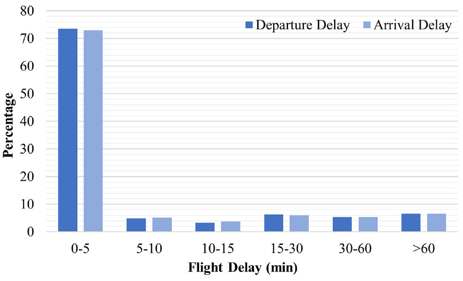
Distribution of flight departure and arrival delays.
Independent Variables
Airline delay variables are augmented with a host of independent variables. The variables considered in this study are chosen based on variables considered in earlier research and on our judgment. We significantly improve flight data for delay analysis by preparing high-resolution weather and traffic condition data in our study. A detailed description of the variable generation process by variable group follows.
Airport-Level Traffic Conditions
Airport-level traffic conditions include air traffic and delay variables at the origin and destination airports. FAA’s ASPM data set provides hourly air traffic and delay information at the airport level. In this study, we aggregate hourly data in the preceding 6 h before the scheduled departure and arrival time of a flight at the origin and destination airports. Airport-level traffic conditions at the origin (destination) airport include scheduled number of departures (arrivals), percentage of on-time gate departures (arrivals), percentage of on-time airport departures, average gate departure (arrival) delay, average taxi-out (-in) delay, and average airport departure delay.
Trip-Level Attributes
Trip-level attributes are mainly sourced from the BTS airline on-time performance data set and include distance and operating carrier. In case of operating carrier, we consider seven major operating carriers including Southwest Airlines, American Airlines, Delta Air Lines, United Airlines, SkyWest Airlines, JetBlue Airways, and other airlines based on the distribution.
Weather Factors
We compile a comprehensive set of weather variables including thunderstorm occurrence, hourly precipitation, visibility, and wind speed at the origin, at the destination, and along the route, sourced from the ASOS data set from Iowa Environmental Mesonet ( 37 ). The weather variable data generation process includes a series of steps. First, the airline route is generated for every origin–destination (OD) pair considering the shortest geodesic path between the origin and destination. The route generated might not necessarily match the exact proprietary carrier flight path, but it still provides an excellent surrogate route for consideration. Second, we divide the continental U.S. into a latitude–longitude grid of 5 degrees (see Figure 2) and compile hourly weather data from all weather stations within each grid. Third, we identify weather conditions at the origin airport during flight departure by aggregating weather data from multiple stations during the departure hour and the preceding 2 h at the origin grid. Similarly, we identify weather conditions at the destination airport considering weather conditions during the arrival hour and preceding 2 h. Third, we identify the sequence of exact grid units along a route, allowing us to generate the time when a flight passes through a grid and record its corresponding weather condition based on weather stations in the grid. To find the intermediate grid, we first identify the shortest route between origin and destination airports considering geodesic distance. Routes between the airports considered in this study are presented in Figure 2. Then, we identify the direction of a flight in respect of grids using distance between origin airport and centroids of intermediate grids. In our processed data set, the number of intermediate grids between origin and destination airports varies from 0 to 11 (higher number of grids for longer flights). Finally, we allocate flight duration based on the distances between origin airport and grids’ cut points to determine the hour of passing and the corresponding weather condition. This process allows us to generate weather conditions during the entire flight. It is important to note that the proposed model system is flexible to accommodate for varying numbers of intermediate grids for flights.
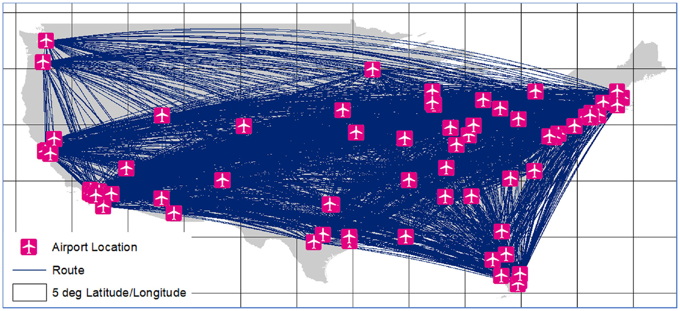
Grid system and routes between the airports.
To illustrate the whole process, we describe the weather variable generation process in Figures 3 to 5 for a flight from John F. Kennedy International Airport (JFK) to Seattle International Airport (SEA). Consider a non-stop flight that is scheduled to depart at 6:30 a.m. Coordinated Universal Time (UTC) and arrive at 12:30 p.m. UTC. First, we identify weather conditions (90th percentile wind speed, 90th percentile precipitation, thunderstorm proportion, and 10th percentile visibility across weather stations) in the origin grid at 4–5 a.m., 5–6 a.m. and 6–7 a.m. Similarly, we identify weather conditions in the destination grid for 10–11 a.m., 11 a.m.–12 noon, and 12 noon–1 p.m. Then, we aggregate weather condition measures for the 3 h to estimate origin and destination weather variables (see Figure 3). Second, we identify the shortest route between JFK and SEA and obtain a path of 10 intermediate grids. Now, we rank intermediate grids from 1 to 10 based on distance between JFK and centers of the grids as shown in Figure 4. Third, we estimate the distances of grid cut points from JFK and calculate the average distances of the grids. Based on average distance, scheduled departure time, trip length, and trip duration, we determine the hour when a flight passes a grid (see Figure 5) and identify the weather conditions in each individual intermediate grid.
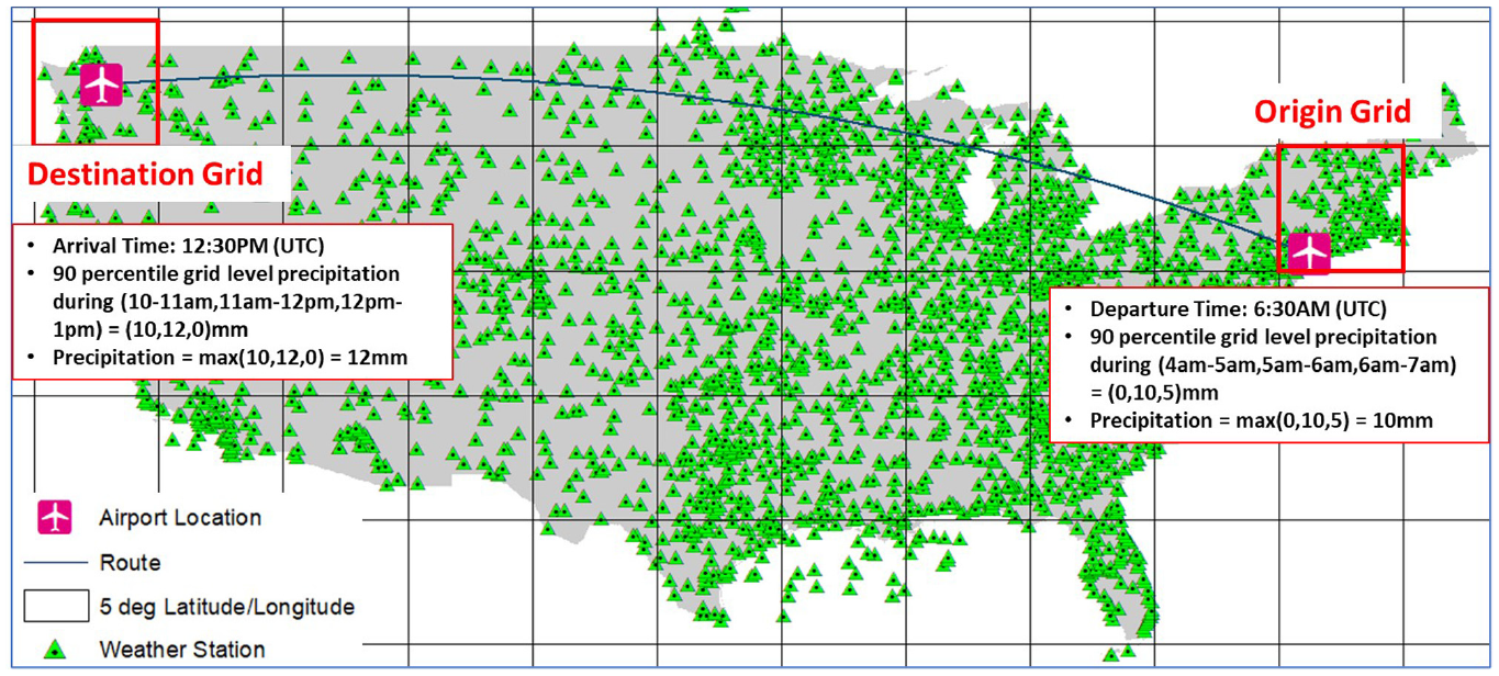
Weather condition at origin and destination airports.
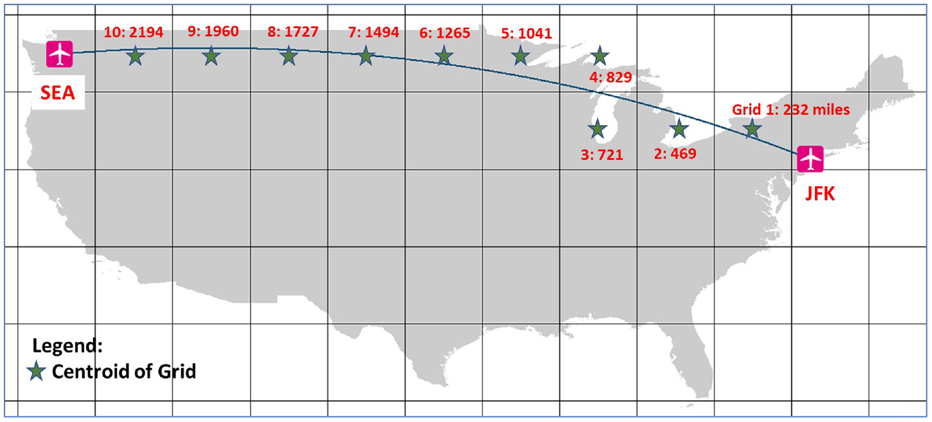
Identification of intermediate grids and their sequence.
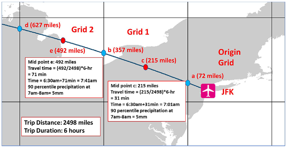
Weather condition estimation at intermediate grid.
Spatial Factors
We consider the location of origin and destination airports in U.S. regions including South, Northeast, West, and Midwest.
Temporal Factors
In this current study, we also investigate the presence of any temporal variability in flight delays. We consider different temporal variables including time of the day, day of the week, and season.
Table 2 offers the summary statistics (minimum, maximum, and average values for continuous variables; frequency for categorical variables) of the considered exogenous variables for the estimation sample. It is important to note that given the varying number of grids, there is no good way to provide a summary of route-level weather data that is representative of the sample. Therefore, we provide descriptive statistics of route-level weather variables across all grids by flight.
Descriptive Statistics of Independent Variables
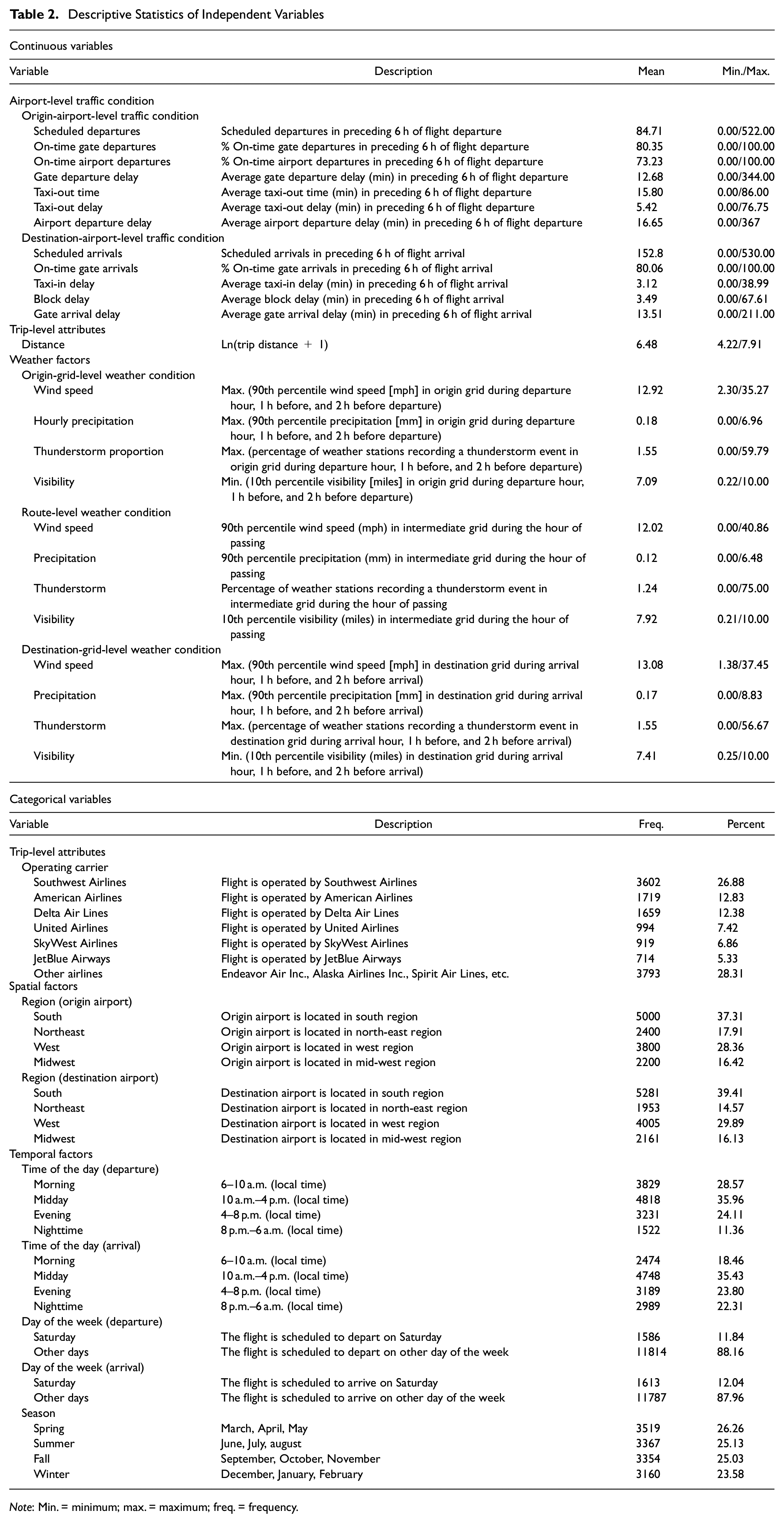
Note: Min. = minimum; max. = maximum; freq. = frequency.
Analysis and Results
Model Selection
The empirical analysis involves the estimation of models by using six different copula structures: (a) FGM, (b) Frank, (c) Gumbel, (d) Clayton, (e) Joe, and (f) Gaussian copulas. A series of models are estimated, and the best data fit is chosen based on Bayesian information criterion (BIC) (see Figure 6). First, an independent copula model (separate GGOL models for flight departure delay and arrival delay) is estimated to establish a benchmark for comparison. Second, we recognize that arrival and departure delay models have similar coefficients for three origin and destination grid weather variables (wind speed, precipitation, and thunderstorms). Therefore, we estimate a restricted version of the independent copula model where we restrict the three origin and destination grid weather variables to be the same across departure and arrival delays. The restricted model offers improved fit relative to the unrestricted model under BIC. Third, six different models considering six copula dependency structures across departure delay and arrival delay are estimated. Based on log-likelihood (LL) and BIC measures, the Joe copula dependency structure provides the best fit. Subsequently, the copula profile of the selected Joe model has been parameterized (see Equation 8). The parameterized Joe copula model shows improved data fit in respect of the BIC measure. Further, the LL ratio test yields a statistical value of 20.64 which is substantially larger than the critical value (= 9.21) with 2 degrees of freedom at 99% confidence level. Therefore, the Joe copula model with parameterization of the copula profile is selected as the final model. It is important to note that we investigated random effects of the variables and we found one random parameter offered a statistically significant result. However, the model with the random parameter does not improve the BIC value of the model compared with the BIC value of the model without the random parameter. Therefore, we did not consider the model with the random parameter as our final model.
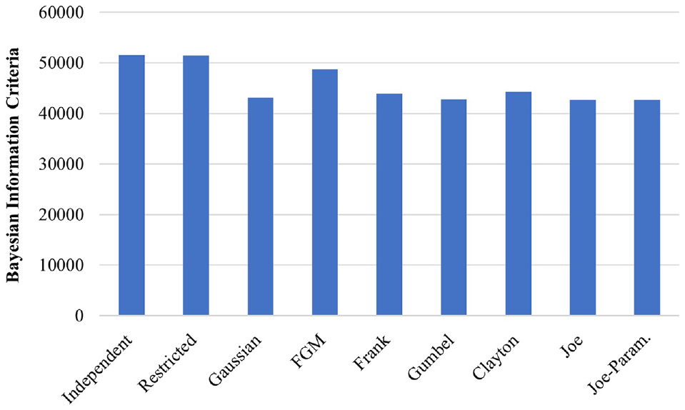
Comparison of alternative models.
Readers should note that the sample size employed in the modeling can be possibly biased. Therefore, before finalizing the model results, we have conducted a rigorous examination of the model performance based on different samples. The analysis procedure and results are included in the supplementary materials. The results illustrate that our model estimation results are stable and quite representative of the data.
Estimation Results
In this subsection, we discuss estimation results from the joint copula model with Joe copula dependency (with parameterization).
Airport-Level Traffic Conditions
Airport-level traffic conditions at origin and destination airports are found to be significantly associated with flight departure and arrival delay, respectively. Among the variables considered in the analysis, number of scheduled departures and average gate departure delay at the origin airport during the 6 h previous to a flight affect departure delay while average gate arrival delay at the destination airport during the 6 h previous to flight arrival affects arrival delay. The estimation results show that an increased level of scheduled departures and gate departure delay at the origin airport increases the likelihood of a flight being delayed. Similarly, increased average gate arrival delay at the destination airport increases the likelihood of a flight being delayed. This result is very intuitive in that adverse traffic conditions at the origin and destination airports mostly trigger flight delay.
Trip-Level Attributes
Among trip-specific factors, trip distance and operating carrier have a significant effect on flight delay. Interestingly, we find the influence of trip distance on the departure delay only. The results indicate that departure delay increases with increased trip distance in general. It is an interesting finding that only departure delay is influenced by trip distance. It is plausible that longer flights have more opportunity to compensate for any initial delay by adjusting their route, a mechanism called “direct routing” ( 38 ). Given this flexibility, it is possible that airports alter the departure times of flights with longer distance more often than other flights. Among operating carriers, we find Delta Air Lines to provide the best on-time performance as indicated by the negative coefficient on both departure and arrival delay. Further, the parameter estimates also suggest reduced departure delay if the flight is operated by United Airlines and SkyWest Airlines. For arrival delay, flights operated by American Airlines, JetBlue Airways, and other airlines are susceptible to longer delays, as indicated by the positive coefficient in Table 3.
Parameter Estimates of Delay Model
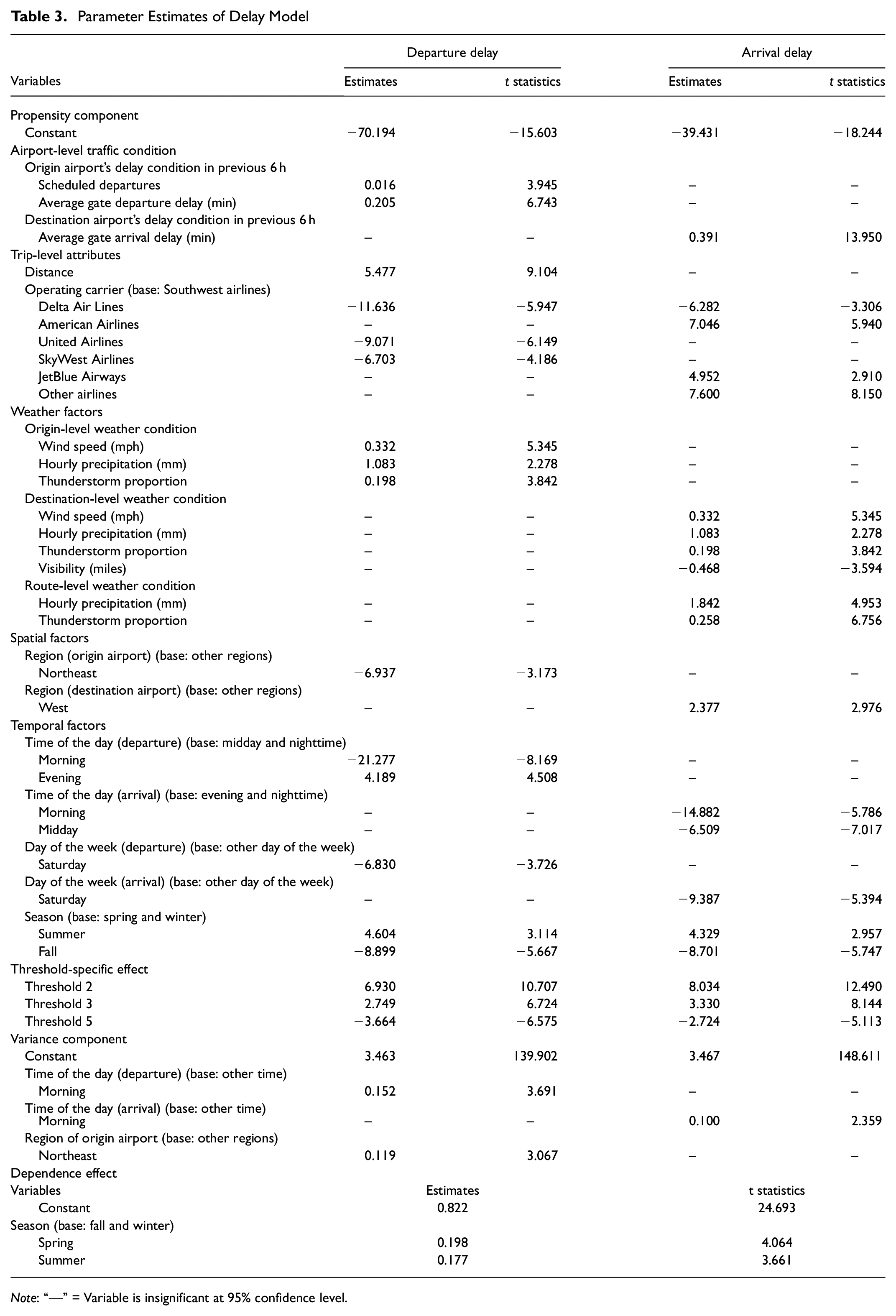
Note: “—” = Variable is insignificant at 95% confidence level.
Weather Factors
The results corresponding to the weather factors highlight the important role of weather in flight delay (both departure and arrival). In this current study, we consider three sets of weather variables: origin level, along the route, and destination level. Origin-level weather factors are considered in the departure delay component. On the other hand, route-level and destination-level weather variables are considered in the arrival delay component. As discussed earlier, effects of the corresponding origin-level and destination-level weather variables (same effect for wind speed on departure and arrival delay; similar too for hourly precipitation, and thunderstorm proportion) are restricted to be the same for departure delay and arrival delay. All the weather-level variables offer expected trends for both departure and arrival delay. For instance, if adverse weather conditions exist at or near the origin/destination airports—including higher precipitation, higher wind speed, and higher frequency of thunderstorm—a flight will be more likely to experience increased departure and arrival delay, which is intuitive. Further, our results also underscore the association of visibility with the arrival delay. As expected, a decreased level of visibility near the destination airport causes increased arrival delay. Under adverse weather conditions, flight operators are unlikely to operate under optimal conditions, affecting flight speed and landing operations. It is important to note that effects of intermediate-grid-level weather variables are accommodated in the arrival delay model. The number of intermediate grids between origin and destination airports varies from 0 to 11. So, the maximum number of weather variable columns is 22 (2 significant weather factors * 11 intermediate grids). For example, a flight from JFK to SEA has 11 intermediate grids and will have 11 potential non-zero values for precipitation (mm) for the 11 grids (grid1, grid2, …., grid11). On the other hand, a flight from Tucson International Airport (TUS) to SEA has only three intermediate grids and therefore only three potential non-zero values of precipitation. It should also be noted that for each weather indicator, we estimate a single effect across all intermediate grids. The results indicate that intermediate-grid-level hourly precipitation and thunderstorm proportion have a significant positive impact on arrival delay, indicating the higher likelihood of arrival delay with an increased amount of precipitation and thunderstorm along the route (as expected).
Spatial Factors
The influence of spatial factors (such as location of origin and destination airports) represents factors specific to these airports that are usually unobserved by the analyst. For example, the airport crew hours and shifts are likely to be similar in a region and thus can positively or negatively affect delay. The exact details of these variables are not easy to obtain. Therefore, they are accommodated through regional and temporal indicator variables. It is evident from estimation results that flight delay is closely associated with the location of origin and destination airports. Flights departing from airports located in the Northeast region in the U.S. experience less departure delay than do flights from other regions in the U.S. (when all other factors are the same). For the arrival delay model component, we observe that flights destined for airports in the West region experience increased arrival delay compared with airports in other regions (when all other factors are the same).
Temporal Factors
Among the temporal factors considered in this study, time of the day, day of the week, and season are significantly associated with flight delays. In general, departure delay is found to be less in the morning time period and higher in the evening time period than at nighttime and midday even after controlling for scheduled arrivals and departures. On the other hand, arrival delay is found to be lower in the morning and midday periods than at other times of the day. From the parameter estimates, we found effects of day of the week and season consistent across departure and arrival delay. Results show that departure and arrival delays are lower on Saturday than on other days in a week. It is also evident that both departure delay and arrival delay are more frequent in the summer season and less frequent in the fall season relative to delays in winter and spring seasons.
Threshold-Specific Effects
The proposed delay model also accommodates for threshold-specific effects on various predefined thresholds. The estimation results of these parameters are reported in the second-row panel of Table 3 and have no substantive interpretation.
Variance Components
We estimate variance of delay model components as a function of exogenous variables. From the results, it is evident that the morning time period variable contributes to the variance profiles of both departure and arrival delay models. Specifically, morning time period delay is subject to a higher variance relative to delay in other time periods. Additionally, the Northeast region variable affects the variance component of the departure delay model. The significance of such factors indicates the presence of heteroscedasticity in the delay data.
Dependence Effects
As indicated earlier, the estimated GGOL model based on Joe copula with parameterization provides the best fit incorporating the correlation between departure delay and arrival delay. The result of the dependency profile is presented in the Dependence effect panel of Table 3. The results clearly highlight the presence of common unobserved factors affecting departure delay and arrival delay. Joe dependency is found positive, indicating upper tail dependency between departure and arrival delays. Such correlation indicates that unobserved factors modifying the likelihood of higher-level departure delay categories also modify the likelihood of higher-level arrival delay categories. Among the various variables considered, we found that the season variable affects the dependence structure. Specifically, the results indicate a stronger dependence between departure and arrival delay during spring and summer seasons.
Model Validation
To test the predictive performance of the proposed model, we perform a validation exercise with the 6700-record holdout sample. For testing the predictive performance of the copula model and its independent counterpart, 25 data samples of 500 records each are randomly generated from the holdout validation sample. The average LL and BIC scores for the proposed copula model are −807.81 [−824.98, −790.63] and 1895.27 [1860.92, 1929.62], respectively. The average LL and BIC scores for the independent model (with restriction) of departure and arrival delays are −968.54 [−987.24, −949.85] and 2235.39 [2198.01, 2272.77], respectively. The validation results clearly highlight the superiority of the proposed copula model over independent models (see Figure 7). Further, we evaluate the performance of the model on training and testing data sets by comparing average LL values. The average LL values on training and testing data sets are −1.58 and −1.59. These numbers clearly indicate that the model fit is quite similar for both data sets. Finally, we compare predicted shares of delay categories with observed shares for the validation sample. The comparison results are presented in Figures 8 and 9. From the figures, we can clearly see that predicted shares of delay categories are very close to the observed shares.
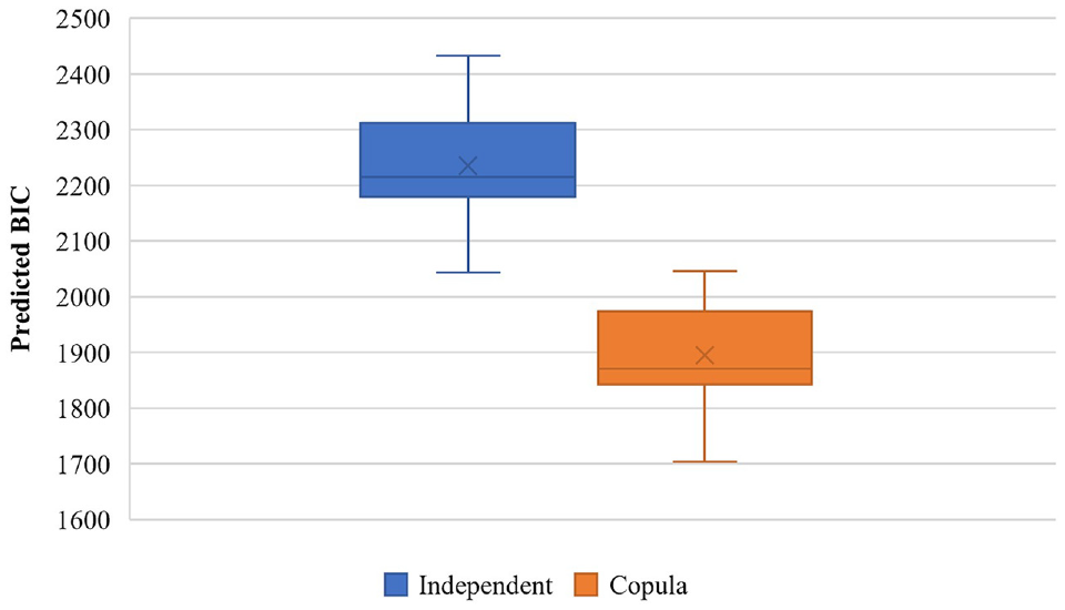
Comparison of predictive performance of two models.
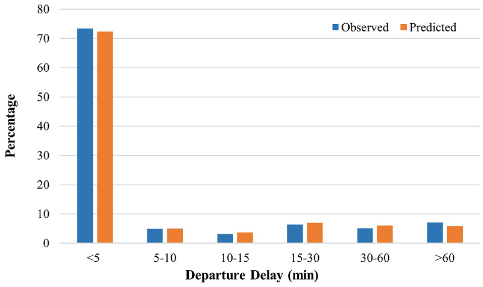
Comparison of predicted and observed share of departure delay.
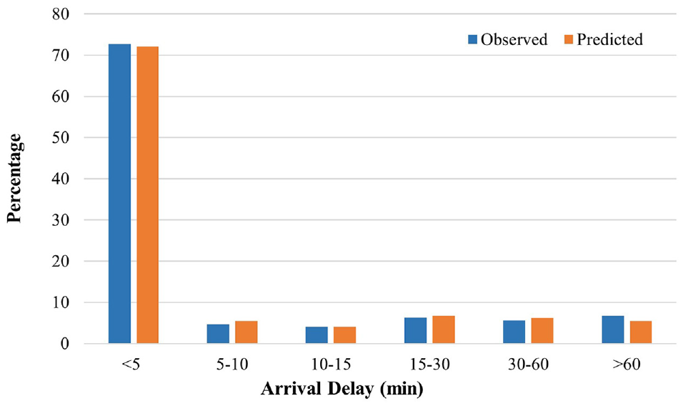
Comparison of predicted and observed share of arrival delay.
Model Illustration
Parameter estimates from Table 3 do not directly provide the magnitudes of the impacts of various independent variables. To illustrate the impact of independent variables, we compute the probability changes of both departure and arrival delay categories for bidirectional flights between an OD pair. We estimate probability of flight delay based on five hypothetical scenarios. For these hypothetical scenarios, we consider different weather condition attributes at the origin grid, intermediate grid, and destination grid level. In generating the probability profile, we consider the following conditions:
In these scenarios, the remaining variables are considered to be the same. For ease of presentation, we identify flight delay probability as a two-alternative prediction—delay under 15 min or delay over 15 min. The probability values for delay over 15 min based on the above-mentioned scenarios are plotted in Figure 10. Departure and arrival delay probabilities are plotted for each airport considering bidirectional flights. For example, departure and arrival delay probabilities are plotted for JFK considering flights to and from Los Angeles International Airport (JFK–LAX and LAX–JFK). From the plots, we can clearly see that probability of delay increases with adverse weather conditions with a probability of arrival delay increasing to about 30%. Among the impact of weather variables we consider, precipitation is found to have the highest influence on flight delay while thunderstorm proportion has the least influence. It is also evident that route-level weather conditions affect arrival delay, not departure delay. It is important to note that these plots are illustrations for the chosen hypothetical scenarios and can be easily generated for different values of independent variables. The reader should note that these plots are provided for demonstrating how the proposed model can be applied at a flight level and the results are likely to vary significantly based on the base scenario under consideration.
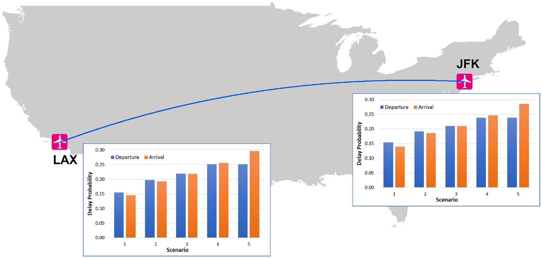
Departure and arrival delay probability based on hypothetical scenarios.
Conclusion
The main focus of the current study is to identify the key factors affecting airline delay by modeling departure and arrival delays at the flight level. This study makes several contributions to airline delay literature. The first contribution of the current study arises from data enhancements for the delay analysis. The main data source of the current study is the 2019 marketing carrier on-time performance data compiled by BTS. The variables processed from the BTS data set are augmented with a comprehensive set of independent variables sourced from secondary data sources including the ASOS data set and the ASPM data set. Using the ASOS data set, we prepare a comprehensive set of weather variables for the entire flight duration near the origin airport, along the flight route, and near the destination airport. Also, we process ASPM data to determine the traffic conditions at the origin and destination airports in the hours preceding the flight departure and arrival. The current research also contributes to airport departure and arrival delay analysis by developing a novel copula-based GGOL model. The proposed model accommodates for the influence of common observed and unobserved effects on flight departure and arrival delays. In our analysis, we employ six different copula structures—the Gaussian copula, the FGM copula, and a set of Archimedean copulas including Frank, Clayton, Joe, and Gumbel copulas.
We compare the predictive performance of independent models of departure and arrival delays and the proposed joint model with different dependency profiles. Based on the model fit measures, the Joe copula model with parameterization provides the best result. The final model indicates that flight delay is significantly influenced by airport-level traffic conditions, trip-specific factors, weather factors, spatial factors, and temporal factors. We test the predictive performance of the proposed model by performing a validation exercise with a holdout sample. The results illustrate the superiority of the proposed model system. Finally, to illustrate both the potential applicability of our model system and the impact of independent variables, we generate the probabilities for arrival and departure delays under a host of hypothetical scenarios for one bidirectional OD pair. The generated airport-level delay probabilities provide a framework for airlines and airports across the nation, to evaluate departure and arrival delay possibilities for their flights based on current weather predictions. The delay analysis can offer potential strategies to improve boarding, deplaning, and luggage handling of flights (identified in advance to have a delay) to improve on-time departure or quick turnaround for the next flight.
To be sure, the current study is not without limitations. In this study, we process weather variables at 5 degree latitude/longitude resolution. It would be interesting to examine whether a finer resolution analysis can improve the accuracy of the model by considering more localized weather data. The data set available to us can also be improved with airline-carrier-specific route information to enhance the weather data collection process and contribute to an improved model. Moreover, a comparison of the developed model with machine learning approaches would be an interesting avenue for future research.
Supplemental Material
sj-docx-1-trr-10.1177_03611981221130031 – Supplemental material for Flight-Level Analysis of Departure Delay and Arrival Delay Using Copula-Based Joint Framework
Supplemental material, sj-docx-1-trr-10.1177_03611981221130031 for Flight-Level Analysis of Departure Delay and Arrival Delay Using Copula-Based Joint Framework by Sudipta Dey Tirtha, Tanmoy Bhowmik and Naveen Eluru in Transportation Research Record
Footnotes
Acknowledgements
The authors would like to acknowledge the Bureau of Transportation Statistics (BTS) and Iowa Environmental Mesonet (IEM) for providing access to their data sets.
Author Contributions
The authors confirm contribution to the paper as follows: study conception and design: Naveen Eluru, Tanmoy Bhowmik, Sudipta Dey Tirtha; data collection: Sudipta Dey Tirtha, Tanmoy Bhowmik, Naveen Eluru; analysis and interpretation of results: Sudipta Dey Tirtha, Tanmoy Bhowmik, Naveen Eluru; draft manuscript preparation: Sudipta Dey Tirtha, Tanmoy Bhowmik, Naveen Eluru. All authors reviewed the results and approved the final version of the manuscript.
Declaration of Conflicting Interests
The author(s) declared no potential conflicts of interest with respect to the research, authorship, and/or publication of this article.
Funding
The author(s) received no financial support for the research, authorship, and/or publication of this article.
Data Accessibility Statement
Data will be shared on request.
Supplemental Material
Supplemental material for this article is available online.
References
Supplementary Material
Please find the following supplemental material available below.
For Open Access articles published under a Creative Commons License, all supplemental material carries the same license as the article it is associated with.
For non-Open Access articles published, all supplemental material carries a non-exclusive license, and permission requests for re-use of supplemental material or any part of supplemental material shall be sent directly to the copyright owner as specified in the copyright notice associated with the article.