
Abstract
Microscopic traffic simulation is vital to assess the performances of various traffic operation and management schemes. Microscopic traffic simulation is usually not parameter-free, and it relies on independent parameters to predict traffic evolution. Thus, parameter calibration is indispensable to conveying trustworthy simulation results. Heuristic algorithms are widely used for parameter calibration. Its logic is for achieving iterative optimization through continuous trial-and-error simulations. This process is time-consuming and usually takes several hours, making the calibration unable to meet the requirements of speed and efficiency. In recent years, parallel computing technology has been gradually applied in the engineering realm, which makes rapid calibration possible. Following the three steps of parallel framework selection, algorithm bottleneck identification, and subtask load balancing, this paper designs and implements the parallelization of genetic algorithm and particle swarm optimization (PSO) calibration algorithms. Finally, the proposed parallel framework is applied to simulation parameter calibration of a section of a 5 km long highway in Australia, and the effectiveness of parallel computing is evaluated from the two dimensions of reduction in calibration computational time and scalability. The results show that the proposed parallel calibration algorithm can shorten the 5 h calibration process to less than 1 h, reducing the calibration time by 80%. The parallel PSO calibration algorithm has better scalability, and its acceleration effect is better when more processors are used.
Micro-traffic simulation has become a necessary technical support tool to assess and predict the performances of various traffic operation and management schemes. In the microscopic traffic simulation model, the driver behavior, the characteristics of traffic flow, and the operation of the traffic system are all described by the calculus of many internal independent parameters, so the ability of the simulation model to reproduce the actual traffic flow mainly depends on the value of the parameters. Micro-traffic simulation platforms often set default values of parameters based on the traffic flow characteristics of the country where the platform is developed. However, these default values often do not match with the specific application scenarios, resulting in low simulation accuracy. Therefore, in practical applications, parameter calibration has become a prerequisite for all subsequent works.
The parameter calibration of microscopic traffic simulation is essentially a combined optimization problem with multiple objectives. The trial-and-error method, proxy models, and heuristic algorithms have been used to solve this essential engineering problem. Gardes et al. and Gomes et al. used the trial-and-error method to calibrate the PARAMICS and VISSIM simulation models ( 1 , 2 ). This kind of method is only suitable for small-scale road networks. The calibration process is highly subjective, resulting in low efficiency.
Some researchers used the proxy model to calibrate the parameters. Osorio and Punzo proposed a simulation-based meta-model calibration method ( 3 ). This method used the structural information of the problem to establish an analytical approximation of the input-output mapping between the calibration parameters and the simulation output. Ištoka Otković et al. applied the neural network to the parameter calibration of microscopic traffic simulation ( 4 ). They used the neural network to replace the process of simulation evaluation. These methods are currently often used for the simulation and calibration of large and complex networks ( 5 , 6 ).
At present, compared with other methods, heuristic algorithms such as genetic algorithm (GA) and particle swarm optimization (PSO) have been more widely used. Siddharth and Ramadurai adopted elementary effects to perform sensitivity analysis and realized simulation parameter calibration based on GA ( 7 ). Focusing on heuristic optimization algorithms, Abdalhaq and Baker compared the calibration effects of GA, tabu search, PSO, and simultaneous perturbation stochastic approximation (SPSA) based on the Simulation of Urban Mobility (SUMO) ( 8 ). Experimental results showed that the SPSA algorithm had certain limitations with regard to parallelization, while PSO could be highly parallelized, and thus they had good potential in solving high-latitude problems. The application of the heuristic algorithm, which derives the optimal combination through iterative evolution, speeds up the process of parameter calibration to a certain extent.
However, the heuristic algorithm realizes iterative optimization through continuous trial-and-error simulation, which is very time-consuming, making the calibration based on the heuristic algorithm unable to meet the requirements of time cost and efficiency. To make the accuracy of the simulation model reach an acceptable level, it still takes several hours ( 7 – 9 ).
In recent years, with the popularity of multi-core computers, parallel computing technology (PCT) has gradually become a research hotspot in the computer field. Parallel computing divides the problem into subtasks and solves them on multiple processors at the same time. It has been successfully applied in fields such as big data mining and the modeling of complex phenomena, and improves the computational efficiency of programs ( 10 – 13 ).
There has been research on applying PCT to parameter calibration in recent years. Hou and Lee proposed a multi-threaded optimization quasi-Monte Carlo (QMC) particle swarm calibration method, realizing parallel computing ( 9 ). However, their research focused on the application of QMC sampling. The proposed QMC is an efficient and robust method that allows modelers to filter out redundant samples and find the global optimum in time. Dadashzadeh et al. applied PCT to the heuristic algorithm by realizing the parallel of loop sentences, and then developed a fast calibration strategy ( 14 ).
However, the studies so far still have the following problems. First, these studies only realized simple applications of parallel computing, without consideration of the entire algorithm design from the perspective of parallel computing. Secondly, researchers only focused on the reduction of calibration computational time when evaluating the efficiency improvement of parallel computing. In fact, when computing resources increase, different parallel computing algorithms obtain different acceleration capabilities; this ability to utilize the increased computing resources is named “scalability.” A comprehensive parallel computing efficiency evaluation system that takes into account the reduction of computing time and the scalability of the algorithm itself has been missing for a long time.
Therefore, this paper applies PCT to the parameter calibration of microscopic traffic simulation. To make up for the shortcomings of the current research, as summarized above, our work is as follows:
Following three steps of parallel framework selection, computing bottleneck identification, and load balancing design, the parallelization of the GA and PSO are designed and implemented to realize parameter calibration.
A SUMO simulation model containing high-density traffic flow is used, and the established parallel algorithms are applied to the simulation model for verification, which proves the effectiveness of the algorithms’ accuracy and efficiency.
The performance of parallel computing on the two calibration algorithms is evaluated and compared from both dimensions of calibration computational time and scalability.
The rest of this article is organized as follows. In the Problem Formulation section, the mathematical problem behind the calibration of micro-traffic simulation models is described in detail from the perspective of objective functions and the parameter space for optimization. The Methodology section introduces the overall framework of the proposed parameter calibration method using PCT. In the Case Study section, based on the SUMO simulation platform, the proposed algorithms are used to calibrate the traffic flow of a section of an expressway in Australia. The findings and conclusions of the experiment are discussed in the Conclusion section.
Calibration Problem Formulation
Objective Function
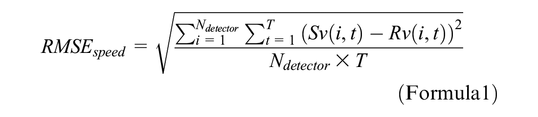
The calibration of micro traffic simulation is essentially a combinatorial optimization problem with objective functions, and the parameters are constrained. The ultimate goal is to minimize the difference between the simulated traffic flow and the actual traffic flow. To make the traffic flow velocity of the simulation model achieve high accuracy, and at the same time simulate the formation and dissipation of bottlenecks in the actual traffic flow as much as possible, this paper refers to the research of Song and Sun (
15
). The root mean square error of the speed (

where
where


where
When the speed value is less than
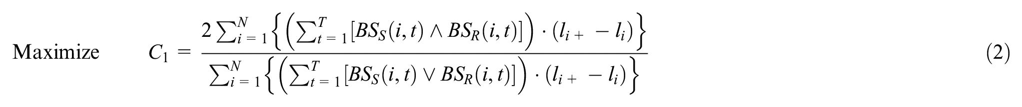
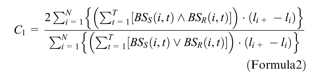
In Formula 2, when
Parameter Space for Optimization
The driving behavior parameters of the SUMO simulation software are mainly divided into three modules: car following model, lane changing model, and speed distribution module. In this paper, the intelligent driver model (IDM) was selected as the car following model, which was first proposed by Treiber et al. based on the generalized force model ( 16 ). IDM has few parameters which are present clear meaning. This model has been widely used, and it often produces consistent results with empirical observations. There are two lane changing models—SL2015 and CL2013—in the SUMO simulation platform ( 17 , 18 ). SL2015 is a sub-lane model, which is only applicable to the simulation scenarios of lane splitting. Therefore, the CL2013 lane change model for lane selection was adopted in this paper.
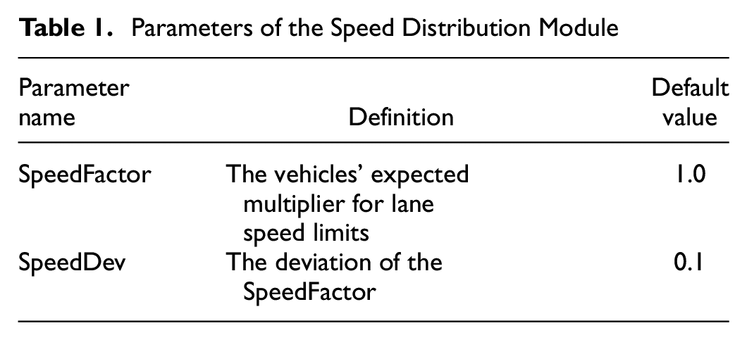
In SUMO, the driving speed of the simulated vehicles is modeled by assigning to each vehicle an individual multiplier which gets applied to the road speed limit. This multiplier is called the “individual speedfactor.” The product of the road speed limit and the individual speed factor gives the desired free flow driving speed of a vehicle. The expected value of the individual speedfactor is denoted as “SpeedFactor,” while, “SpeedDev” represents the deviation of the SpeedFactor. These two parameters form a speed distribution module that controls the sampling of vehicle speed. The specific meanings of the two parameters are shown in Table 1.
Parameters of the Speed Distribution Module
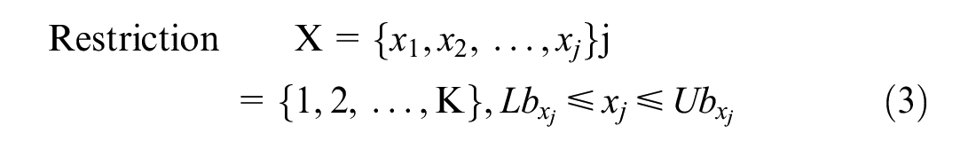
We followed several principles to determine the ranges of the parameters to be calibrated. First of all, the ranges of parameters must comply with the basic regulations of SUMO’s official documents. Secondly, constraints between parameters needed to be considered. For example, from common sense, the value of emergency deceleration would be larger than that of normal deceleration. Then, the ranges of parameters with similar meanings in previous studies also needed to be referred to. Finally, we also refer to the default values given in SUMO, making the ranges around the default values.
After an initial selection, 19 parameters were used for calibration, far exceeding the expected number of calibration parameters. Too many calibration parameters would lead to high dimensionality and computational complexity of the parameter calibration problem. Therefore, to save computing resources and reduce the dimension of the optimization problem, avoiding the trap of local optimal solution, we used the sobol sensitivity analysis to realize the selection of key parameters ( 19 ).
Sobol sensitivity analysis is based on the basic assumption that variance can well represent the uncertainty of the model’s output. This method uses the sobol sequence for sampling, which can be divided into two steps: the value acquisition using sobol sequence and the sample generation.
Sobol sequence is essentially a quasi-random low-discrepancy sequence used to generate uniform samples of parameter space, which is constructed by linear recurrence relations in finite fields. In this paper, we generated a basic sobol sequence matrix
Latin hypercube sampling (LHS) was first described by McKay et al. ( 21 ) in 1979; it is a statistical method for generating near-random samples of parameters from multidimensional distributions ( 21 ). The sampling process of LHS consists of two parts: interval sampling and sample sorting. LHS firstly stratifies the sample space according to the cumulative probability density curves of random variables, then conducts sampling in each sample space. Finally, LHS uses the sorting algorithm to make the correlation between random variables of the sampling result consistent with the one between the real random variables.
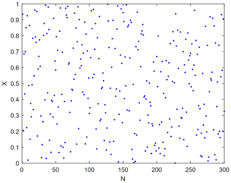
We took the sampling in a one-dimensional sample space as an example. With 300 sample points generated in the X∈[0, 1] interval, the results of sobol sequence sampling are compared with those generated by LHS, which is commonly used, as shown in Figures 1 and 2. The horizontal axis represents the serial number of the sample point. A total of 300 sample points were generated. The vertical axis is the value of the sample point. As can be seen from the figure, sample points generated by sobol sequence sampling are more evenly distributed, with wide coverage and better diversity.
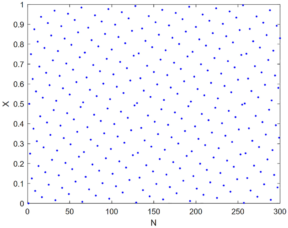
Sobol sampling.
Latin hypercube sampling (LHS) sampling.
After the sample parameter matrix

Within the formula:
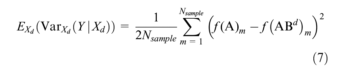

where
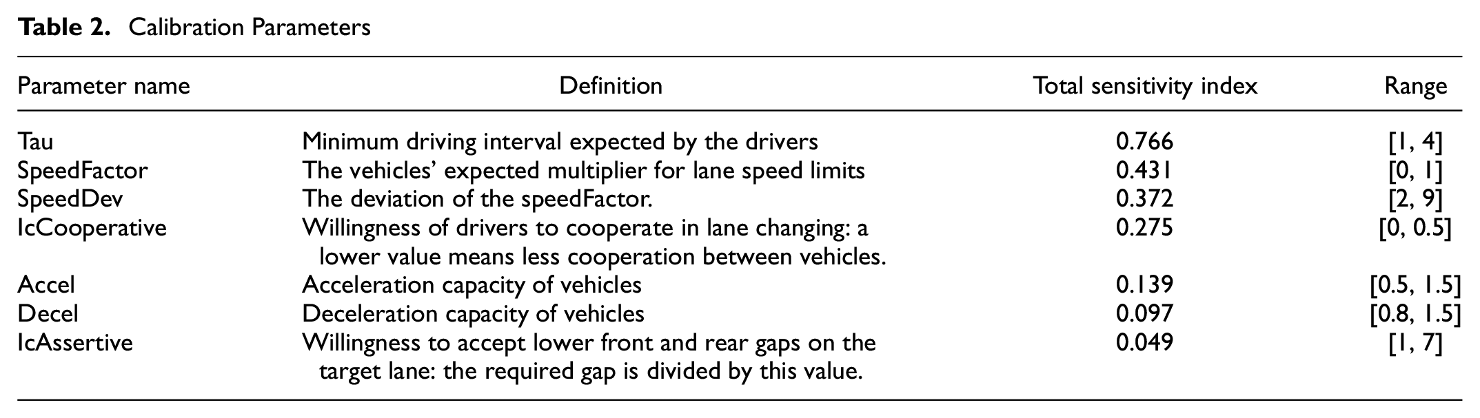
Referring to previous studies, when the global sensitivity index
Calibration Parameters
Methodology
In this section, GA and PSO, which are two classical heuristic algorithms widely used in calibration problems, are presented in detail. Then, the parallel frameworks of the two calibration algorithms are designed and implemented following three steps: the parallel framework selection, computing bottleneck identification, and load balancing design.
Genetic Algorithm (GA) and Particle Swarm Optimization (PSO)
Genetic Algorithm (GA)
GA is a non-deterministic quasi-natural algorithm, first proposed by Holland in 1975 ( 23 ). The GA first composes a certain number of genetically encoded individuals into the initial population. According to the principle of survival of the fittest, individuals are selected to generate new populations according to their fitness. The selected outstanding individuals are combined, crossed, and mutated to achieve individual reorganization. The above process continues to iterate and loop, producing a better approximate solution in the evolution.
The GA used in this article is as follows:
1) The generation of the initial population. We randomly sample within the value range of each parameter to generate the initial population. Then the Gray coding is used to map the parameter sets from the solution space to the search space that the GA can handle.
2) Fitness function. In this paper, the
3) Selection. Based on the fitness values of different individuals, outstanding individuals are selected to produce offspring populations in accordance with the evolutionary principle. This paper adopts the method of tournament selection. We take a certain number of individuals from the population each time, using sampling with replacement, and then select the best one to enter the progeny population. We repeat this operation until the new population size reaches the original value.
4) Crossover. Two individuals for evolution are randomly selected. The same position of the two carries out gene exchange according to the crossover probability
5) Mutation. The mutation operation in this paper is to invert the corresponding bit of the individual code according to the set mutation probability
We repeat the above process until individuals who meet the fitness value requirements are obtained. When designing and selecting the hyperparameters of GA, to ensure the fairness of the comparison, the population size of each generation was determined to be equal to the number of particles in each generation in PSO. We mainly considered the crossover probability
Particle Swarm Optimization (PSO)
The PSO algorithm is a swarm intelligence algorithm proposed by Kennedy and Eberhart ( 24 ). The algorithm regards individuals as random particles, and guides particles to move to the optimal solution through the local and global optima.
We used the PSO algorithm with M particles to solve a problem with a search space of dimension K. In
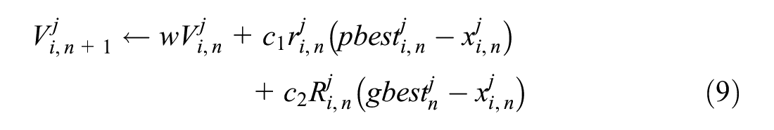
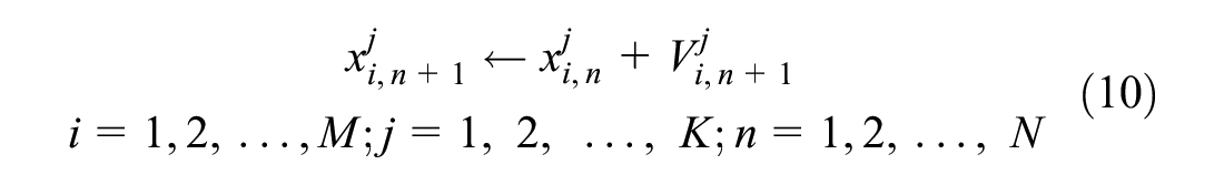
where
(
The vector
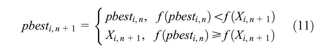
where
f(.) = the objective function to obtain the fitness value of the corresponding position.
The vector
Acceleration coefficients
Parallel Computing Design
The Selection of Parallel Framework
The selection of parallel architecture needs to consider the specific characteristics of the problem to be solved. Problems suitable for PCT often have the following salient features:
The problem can be decomposed into discrete pieces that can be executed concurrently.
The different discrete fragments obtained by decomposition have no requirement on the execution order, which means that they are independent fragments.
The GA calibration process is shown in Figure 3a. The order of execution of these main steps is fixed. The main steps are dependent on each other seriously, meaning that they cannot be parallelized. However, the three steps of running the simulation to calculate fitness, crossover, and variation can be decomposed into independent discrete segments that can be executed concurrently.
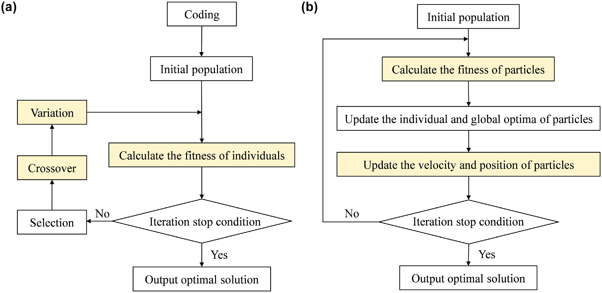
The framework of the calibration algorithm: (a) genetic algorithm and (b) particle swarm optimization.
The main steps of the PSO calibration algorithm are shown in Figure 3b. There is also a strong dependency between the four main parts. The steps of updating the individual and global optima require a lot of communication between particles. Therefore, the two steps of evaluating particle fitness and updating particle position and velocity can be divided into discrete segments that could be executed by PCT.
The computer framework can be divided into four categories from the two dimensions of instruction flow and data flow: single instruction single data (SISD), single instruction multiple data (SIMD), multiple instruction single data (MISD), and multiple instruction multiple data (MIMD). SISD is a serial machine in the standard sense. The other three categories belong to the framework of parallel computing as far as their operation logic is concerned. In the MISD architecture, different processing units can independently execute different instruction streams, but they receive the same single data stream. The SIMD architecture is a typical parallel architecture. All processing units execute the same instruction in any clock cycle, and each processing unit processes different data elements. MIMD is a parallel computing framework in the highest sense, in which different processors can process different instruction streams and different data at the same time.
According to the above analysis of the two calibration algorithms, in the GA and PSO calibration algorithms a certain main step can be divided into discrete segments that are executed concurrently. In these steps, the instructions executed by the discrete segments are the same, and need to be applied to different data, and the results are returned to the main thread for information aggregation. Therefore, in this study, SIMD is an applicable parallel framework.
The Identification of Calculation Bottleneck
This step is to analyze and identify which part of the whole process has completed most of the work of the program, through a program analyzer or performance analysis tool. Based on the results of the analysis, we made the PCT focus on these key points of the program while ignoring the rest that takes up a small amount of Central Processing Unit (CPU) computing resources.
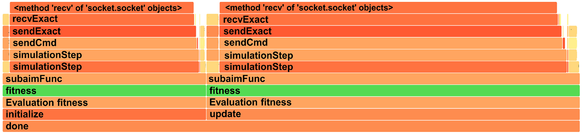
The flame graph is a visualization tool that shows the proportion of CPU computing resources occupied by each function during the program operation. The flame graph is drawn based on the stack traces, which list all the functions being executed by the CPU at any given time. The flame graph shows the time distribution of program execution from a global perspective. Each column represents a call stack, and the bar is used to represent a specific function. The vertical axis arranges functions from bottom to top according to the calling relationship. On the horizontal axis, the flame graph aggregates many call stacks in alphabetical order, which does not represent a chronological order.
The length of each bar represents the frequency of occurrence of the function in the sample. Therefore, the longer the bar, the longer the execution time of the function, which is most likely to be the calculation bottleneck of the algorithm.
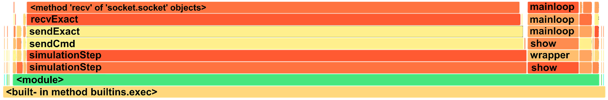
When both algorithms run for two generations and simulate five times for each generation, the flame diagrams of the GA calibration algorithm and the flame diagram of the PSO calibration algorithm are shown in Figures 4 and 5. It can be seen from the graphs that the SimulationStep function of the two calibration algorithms occupies most of the computing resources during the entire calibration process, which is extremely time-consuming. The SimulationStep function writes the generated parameter sets into the SUMO simulation platform and controls the simulation model by using Traffic Control Interface (TraCI), which is a traffic control interface that realizes the interaction between SUMO and external control algorithms. The interactions implemented in this article include controlling the start of the simulation and acquiring data in the SUMO traffic simulation environment. Therefore, based on the results of the flame graph analysis, we applied PCT to the SimulationStep function in the GA and PSO calibration algorithms, which means to realize the parallelization of simulation operation and the calculation of evaluation indexes. The structures of the two parallel calibration algorithms are shown in Figures 6 and 7.
Flame diagram of single-thread genetic algorithm calibration.
Flame graph of single-thread particle swarm optimization calibration.
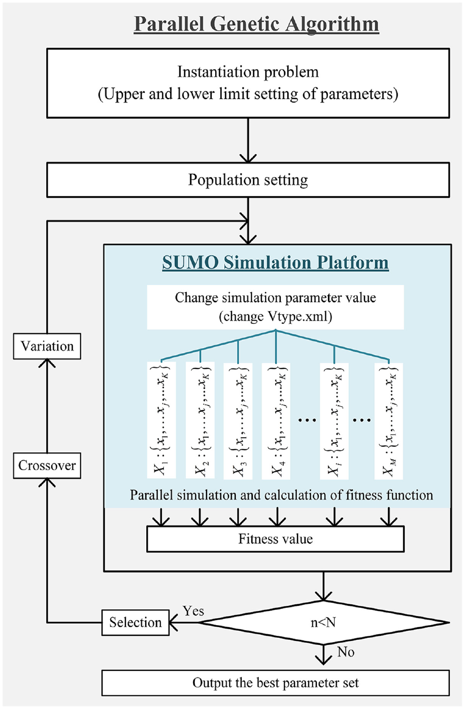
Framework for parallel genetic algorithm calibration.
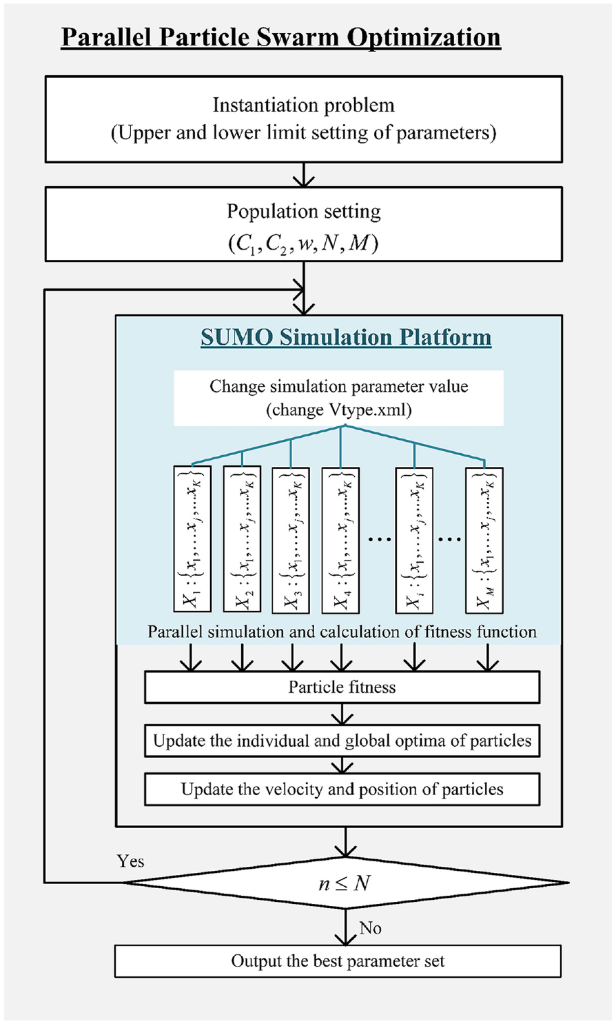
Framework of parallel particle swarm optimization calibration.
The Realization of the Subtasks’ Load Balancing
After the first two steps, the frameworks of the GA and PSO parallel calibration algorithm have been built. According to the characteristics of discrete segments, this step considers the design of load balancing for parallel computing. “Load balancing” refers to distributing approximately equal amounts of computing work on each processor, so that all processors remain busy at all times, minimizing the idle time of all processors. Load balancing is an important performance indicator of parallel programs. There are two main methods to realize load balancing of parallel computing: equal distribution of tasks and dynamic task distribution.
In the calibration problem of the microscopic traffic simulation model, the parameter combinations are input into the simulation model. Because of the difference in parameter selection, the running time and computational complexity of each simulation are not exactly the same. There are even some cases where the simulation exits because the parameters are too biased. If the method of evenly distributing tasks is adopted in this problem, each processor would run the same number of simulations, making the unbalanced load inevitable.
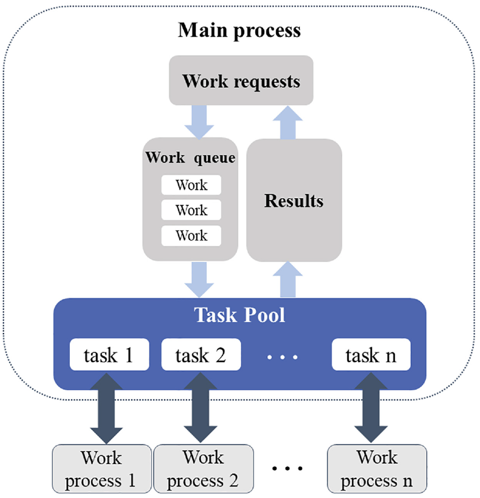
Therefore, in our work, the mode of task pool is tailored to realize the dynamic allocation of tasks, as shown in Figure 8. There are the main process and worker processes in the task pool mode. The main process is the entrance to the program execution, which can be understood as the main function of the program. PCT divides a big problem into small tasks, and the work processes are the program entities that perform the subtasks. Usually, there is only one main process and multiple work processes. The task pool is set with a maximum number of processes and belongs to the main process. When a new work request is submitted to the task pool, if the pool is not full, a new work process will be created to execute the task, but if the number of processes in the pool has reached the upper limit, then the request will wait. Once a certain task in the pool ends, it will enter the task pool and be executed by the work process. This means that the fastest work process will complete more subtasks.
The mode of task pool.
In the context of the heuristic algorithm calibration problem, the subtask is the simulation operation under a certain set of parameters. The execution results returned to the main process are the accuracy evaluation indexes calculated according to the simulation model. The task pool size is the number of computing cores used in parallel computing.
Case Study
This section presents a case study. A simulation model of a 5 km long highway section is built for parameter calibration, based on the SUMO microsimulation ( 28 ). First, the performance of the parallel GA and the parallel PSO proposed is compared from the perspective of accuracy.
More importantly, this paper selects four quantitative indicators to evaluate the efficiency of parallel algorithms from the perspective of calibration computational time and scalability. In the Results Analysis section, the simulation computational time of the calibration algorithms with or without PCT is compared. One step further is that we change the number of processors used in parallel and compare the application effects of PCT on GA and PSO based on the established efficiency evaluation indicators.
Simulation Scenario
The study area is in the upstream and downstream sections of the Deception Bay Street exit ramp and the Anzac Street entrance ramp of the Bruce Expressway in Australia, with a total length of 5 km, as shown in Figure 9. The study area includes basic highway sections, diverge areas, and merge areas. The area where the ramp merges into the confluence area is a typical lane-drop bottleneck.
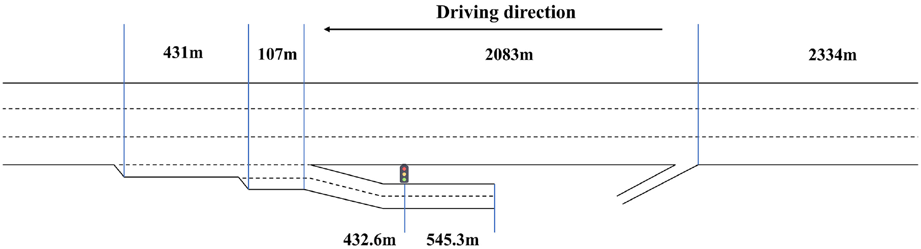
The geometrical schematic diagram of the research section.
Along the study section, there were 10 loop detectors, every 480 m on average. Cross-sectional data such as traffic, speed, and occupancy rate on the main lane could be obtained. This paper selected the field observation data on September 2, 2020, for parameter calibration research. By looking at the field loop detector data, it could be seen that the traffic entering the road segment began to increase sharply at around 5 a.m., and obvious congestion began to appear at the ramp junction at around 6 a.m. and extended upward. After 8 a.m., the congestion began to dissipate. The traffic flow data collected from 6:00–6:59 a.m. was used for the calibration experiments. The formation process of bottleneck congestion was included in the calibration period. The observed heatmap for speed during the calibration period is shown in Figure 10.
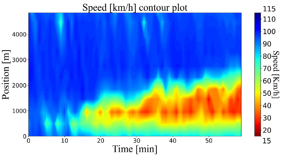
Speed heatmap for mainline (6:00–6:59 a.m.).
Calibration Accuracy Evaluation Indicators
With reference to Song et al.’s research, this paper used two quantitative indicators,
The
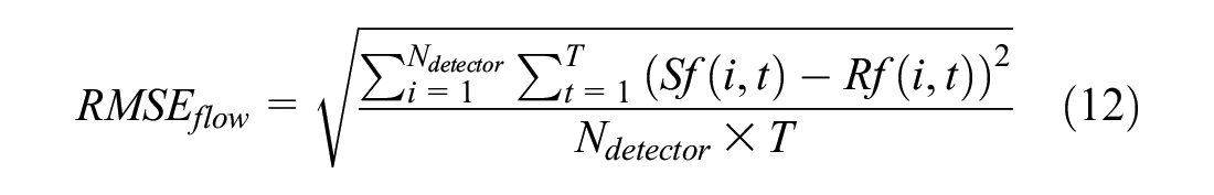
The
where
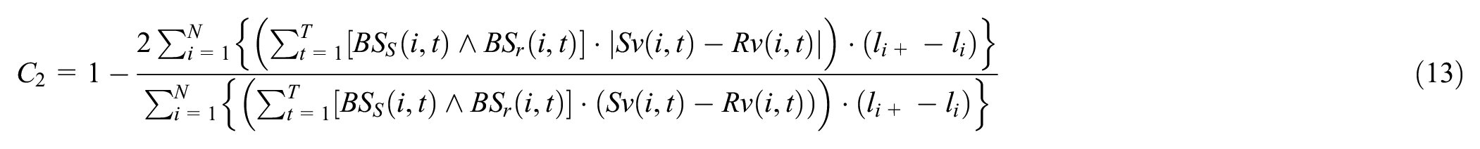
The
where
In addition to the four quantitative evaluation indicators, the accuracy of the simulation model can also be evaluated from an intuitive visual point of view by referring to the speed heat diagram.
Results Analysis
Calibration Result
In the case study, the IDM model was selected as the car-following model, and the LC2013 as the lane changing model. Two indicators of
Table 3 shows the accuracy comparison between the parallel GA and the parallel PSO. Figure 11 shows the speed heatmaps of the two calibration algorithms’ results. When using the default values in the SUMO simulation platform, the simulation model cannot simulate the bottleneck state in the actual traffic flow at all. With reference to speed and flow matching, the calibration result of parallel GA is better than that of parallel PSO. The two index values of
Accuracy Comparison of Calibration Results.
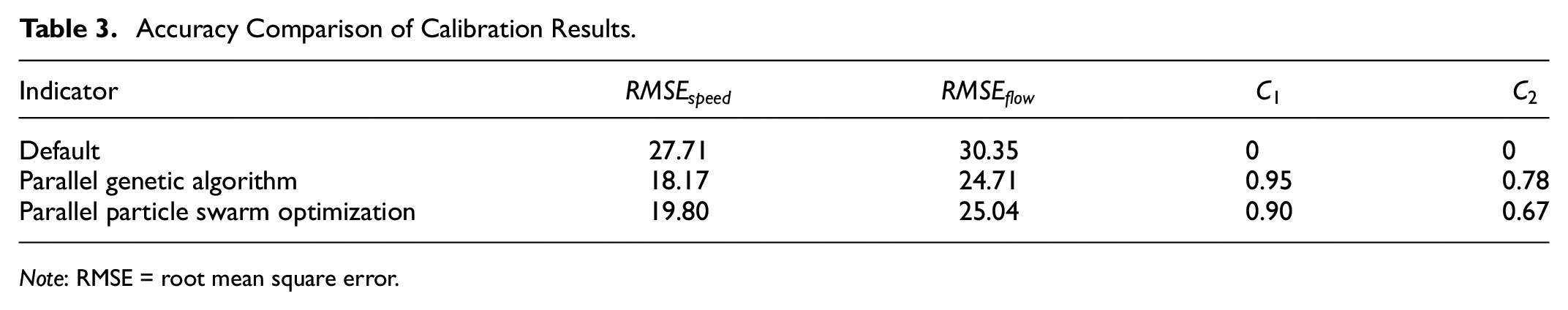
Note: RMSE = root mean square error.
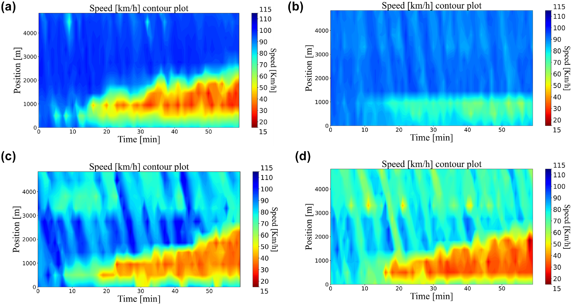
Comparison of speed heatmap: (a) field, (b) default, (c) result of parallel genetic algorithm, and (d) result of parallel particle swarm optimization.
Efficiency Evaluation Indicators of PCT
Based on the accuracy comparison indexes, the accuracy of the parallel calibration algorithms was verified. Concerning the evaluation of the efficiency improvement brought by parallel computing, aside from the commonly used computational time, we considered the ability of parallel algorithms to utilize available computing resources, which was called “scalability.” Thus, the efficiency evaluation indicator system was established based on both the computational time reduction rate and scalability, which included four indicators: calibration computational time, acceleration ratio, parallel efficiency, and algorithm scalability.
1) Calibration computational time. The calibration time in this project is defined as the time of the entire calibration algorithm from encoding to outputting the best results. Calibration time is the most intuitive and simple evaluation indicator for the improvement of calibration efficiency by using parallel calculation. More importantly, the calibration time is also the basic data necessary to calculate other efficiency evaluation indicators, such as acceleration ratio.
2) Acceleration ratio. The acceleration ratio refers to the ratio of the optimal single-thread calculation time of the program to the parallel calculation time using multiple processors. It is the simplest and most widely used metric to detect the performance of parallel algorithms. The parallel acceleration ratio is defined as follows:

where
3) Parallel efficiency. Parallel efficiency is an evaluation index calculated based on the acceleration ratio, which is defined as follows:

The efficiency of parallel computing is affected by the theoretical maximum acceleration ratio
4) Scalability. Scalability refers to the ability of parallel algorithms to increase parallel speed proportionally by adding more computing resources. It is a measure of the extent to which parallel algorithms can effectively utilize the increased capacity of multiprocessors. With the increase of the number of available processors, if the parallel marginal efficiency curve remains basically unchanged or slightly decreases, the scalability of the parallel algorithm is considered to be good. Conversely, if the efficiency curve drops quickly, it is considered that the parallel algorithm has poor scalability.
Results of Calibration Efficiency Experiment
The experiment controlled the evaluation times in parallel GA and parallel PSO calibration algorithms to be the same. When using different numbers of processors in parallel, the calibration computational time, reduction ratio, and parallel acceleration ratio results of the two are shown in Table 4. Figure 12 shows the comparison of the time reduction ratio of parallel GA and parallel PSO calibration algorithms under different numbers of processors. Figure 13 shows the efficiency curves of the two parallel algorithms.
Time Reduction and Acceleration Ratio
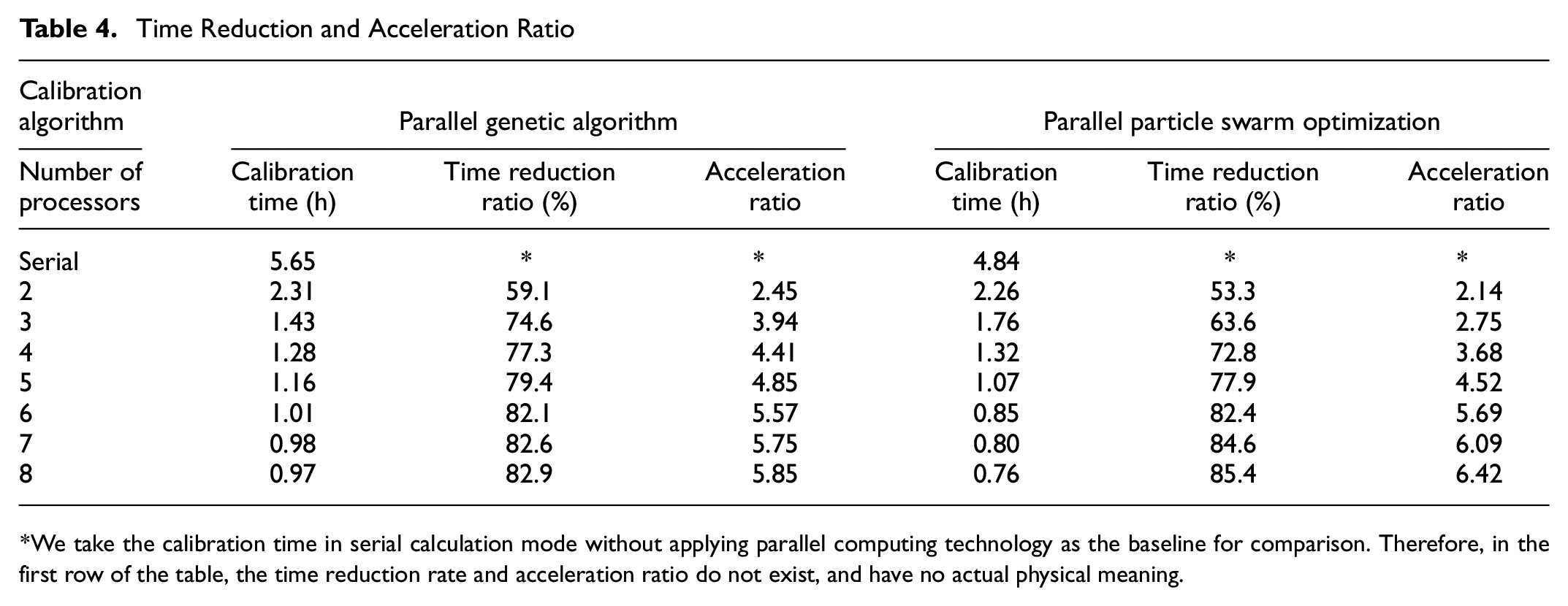
We take the calibration time in serial calculation mode without applying parallel computing technology as the baseline for comparison. Therefore, in the first row of the table, the time reduction rate and acceleration ratio do not exist, and have no actual physical meaning.
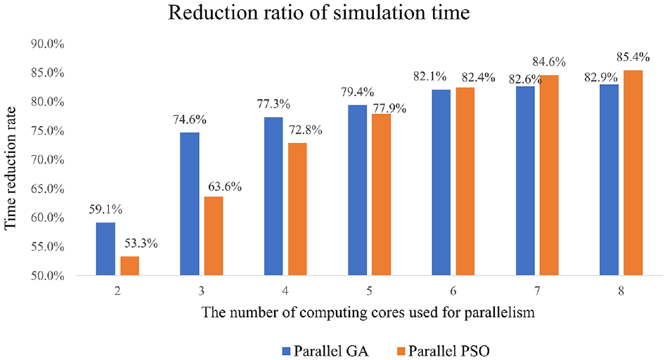
Calibration time reduction ratio.
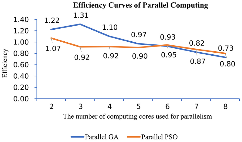
Parallel efficiency curve.Note: GA = genetic algorithm; PSO = particle swarm optimization.
It can be seen from the results that the application of parallel computing greatly shortens the calibration time. In the serial calibration algorithm, the calibration takes 5.65 h. By using PCT, the calibration time is shortened to less than 1 h, and a reduction of 80% is achieved. The experimental results verify the great significance of parallel computing in the calibration problem.
As can be seen from the efficiency curves of the two, the curve of the parallel PSO calibration algorithm is gentler. This shows that its scalability is better, which means its ability to use increased computing resources is stronger. When the number of parallel processors is small, parallel computing has a better acceleration effect on the GA calibration algorithm. For example, when using three processors, the calibration time of parallel GA is reduced by 74.6% compared with serial calibration, while the time reduction rate of parallel PSO is only 63.6%. However, as the number of processors increases, the acceleration effect of parallel computing in the PSO calibration algorithm becomes better. When eight processors are used for parallel computing, the calibration time of the parallel PSO calibration algorithm has been reduced by 85.4%, while the reduction rate of the calibration time in the parallel GA calibration algorithm has stagnated at about 80%. In this case, if the effectiveness of parallel algorithms is compared only from the single dimension of the simulation time reduction ratio, once the number of processors used in parallel alters, the comparison result would be invalid. The result of the case study verifies the necessity of comparing the application effects of parallel computing from the two dimensions of simulation time reduction and scalability.
Conclusion and Discussion
At present, the heuristic algorithm has been widely used in the parameter calibration problem of microscopic traffic simulation, but the calculation bottleneck of the trial-and-error simulation makes it unable to meet the requirements of rapid calibration. PCT can be applied to optimize this computing bottleneck. This paper designs and implements parallel GA and parallel PSO calibration algorithms in accordance with the three steps of parallel framework selection, algorithm bottleneck identification, and subtask load balancing design. When evaluating the application effect of parallel computing, the evaluation indicator system was established from the two dimensions of calibration computational time and scalability.
This research verifies that the application of parallel computing to parameter calibration can greatly speed up the calibration speed, and the acceleration effect reached above 80% in the case study. At the same time, the research results also prove that the ability of parallel algorithms for utilizing increased resources, which is called scalability, is an important and necessary indicator for evaluating parallel algorithms. The evaluation indicator system proposed in this paper from calibration computational time and scalability is reasonable and necessary. As can be seen from the results, the scalability of parallel PSO is better than that of parallel GA.
The findings of this paper have contributed to the rapid calibration of microscopic traffic simulation parameters. It also guides researchers who apply PCT to the calibration problem in the future.
This study also has limitations. The GA and PSO algorithms used in this paper are the most basic forms. At present, both algorithms have been improved a lot, producing many variants with better optimization effects. In future work, we will consider the latest variants of PSO and GA, and consider complex parameter adjustment mechanisms, such as time-varying acceleration coefficients in PSO.
On the other hand, although the PCT used in this paper greatly improved the efficiency of the parameter calibration, the current calibration computational time within 1 h is still far from the requirement of online calibration. In the future, the calibration method based on the proxy model can be combined with PCT to further speed up the calibration process.
Furthermore, verifying the applicability of this scheme to road networks of different scales and comparing the application effects is another worthy research direction. However, because of the lack of field traffic flow data on large-scale road networks, currently we are unable to do further research. As the network size increases, completely different parallel computing schemes can be applied. For example, we can divide the large road network into discrete road segments, and a simulation model of the traffic flow on each segment can be run by different computing cores. The effect of such a parallel scheme will definitely be different from our current scheme. We will take these into account to make a comprehensive, systematic, and scientific research on the application of PCT in the calibration of microscopic traffic simulation models. This paper will be an essential foundation for our future research.
Footnotes
Author Contributions
The authors confirm contribution to the paper as follows: study conception and design: L. Tang, Y. Han, J. Sun; data collection: L. Tang, Y. Han; analysis and interpretation of results: L. Tang, Y. Han, D. Zhang, Y. Tian, J. Sun; draft manuscript preparation: L. Tang, Y. Han, D. Zhang, Y. Tian, A. Fu, L. Yue, H. Zhang. All authors reviewed the results and approved the final version of the manuscript.
Declaration of Conflicting Interests
The author(s) declared no potential conflicts of interest with respect to the research, authorship, and/or publication of this article.
Funding
The author(s) disclosed receipt of the following financial support for the research, authorship, and/or publication of this article: This work is sponsored by National Nature and Science Foundation of China (grant number 52002279).