
Abstract
Understanding the relationship between the built environment and online car-hailing travel behavior can greatly influence sustainable urban development. These complex impacts are not fully understood from a whole-day perspective. This paper took the central urban area of Nanning, China as a case study, and analyzed the data of 1,154,759 online car-hailing service orders collected by the Nanning Information Center over the course of a week. Thiessen polygons based on road networks were used to divide the research area. A partial dependence plot and random forest regression were used to examine the nonlinear impacts of the built environment (home-work attributes, traffic facility attributes, land use, and diversity) on online car-hailing trip demand throughout the day. The results show that the built environment elements that affect the demand for online car-hailing differ at different times of the day and that they have different ranges of influence. For example, residential areas play an important role in the commuter period for demand with a contribution rate of 33.2%, while the contribution rates for the remaining periods are less than 5%. In the whole day, cultural services, health services, leisure sports services, and catering services are important factors. And if there are enough training institutions to form a separate trading area within a city, this will have a profound impact on travel demand. In comparison to subway stations, bus stations contribute more to the demand. The study results will assist the government in improving urban transportation coordination.
Over the past decade, on-demand platform mobile services have been fully developed as a result of rapid advances in information and communication technology. Among the emerging modes of shared transportation, shared bikes, electric scooters, and online car-hailing (OCH) have gained a lot of popularity ( 1 , 2 ). OCH can reduce urban transport emissions if the scale of the service is sufficient to minimize the cruising time of drivers ( 3 ), which demonstrates that shared transportation can reduce urban traffic congestion and pollutant emissions to some extent. Over the past six years, the OCH business has grown rapidly in China, and it plays an important role in people’s travel activities. According to the China OCH regulatory information exchange platform, 214 OCH companies had been granted business licenses in China as of December 31, 2020. As of December 2020, the platform had received 810 million orders ( 4 ). With its flexibility and door-to-door service, OCH can almost match the convenience of private cars, particularly in cases where users go to places where parking is difficult and parking fees are high as OCH not only reduces the need for parking, but also reduces waiting times ( 5 ).
While OCH offers many benefits, its scale in cities must be limited within a reasonable range. It is very important to ensure the load factor. By reducing the vehicle’s empty-loading cruise, we can reduce energy consumption, which further reduces traffic congestion and environmental pollution. Before picking up customers, having a clear understanding of the OCH demand distribution can greatly improve the load factor ( 3 ). In light of this, exploring the urban OCH ridership is an important task, and the research shows that the built environment has a significant impact on transit ridership ( 6 – 8 ) and online car-hailing ( 9 – 14 ). These empirical studies point out that factors related to home-work attributes, land-use density, and diversity and transport facility characteristics all significantly affect the passenger flow.
It is worth noting that our study is different from the previous ones. To distinguish from previous studies, we summarized the main features of relevant past studies, as listed in Table 1. Table 1 indicates that most of these studies explored the linear relationship between environmental factors and travel demand (e.g., least squares, geographically weighted regression, multiscale geographically weighted regression, logistic regression), and the scale of influence on individual environmental factors is limited. In fact, when the built environment features are at different ranges, the impact on passenger flow may also be different ( 15 ). This nonlinear relationship has been demonstrated for other modes of travel (e.g., subway, bus, and walking) ( 6 , 16 , 17 ). In addition, most of these studies neglected to examine the relationship between the two on a time scale (e.g., peak hours were used). Few studies explored it from a full-day perspective and still used the assumption of linearity. It is important to note that such typical analyses may mask important partial information about the impact of a policy change and have limitations in examining its temporal heterogeneity ( 18 ). Last but not least, most of the existing studies have used a spatial grid division method when carrying out the division of study units. This simple and straightforward division ensures consistency of area but ignores the impact of road network distribution on spatial travel.
Characteristics of the Study of the Relationship between OCH and the Built Environment
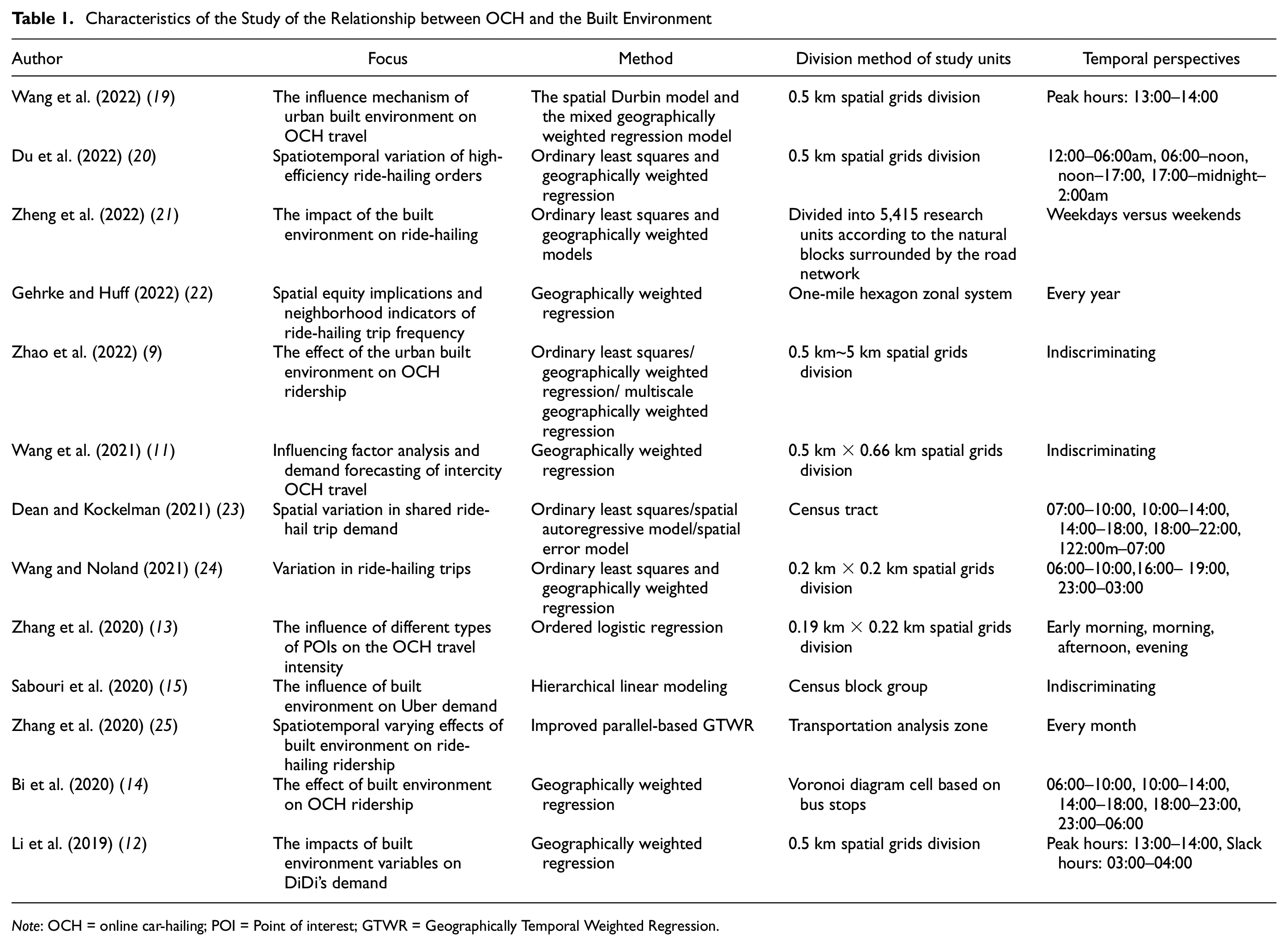
Note: OCH = online car-hailing; POI = Point of interest; GTWR = Geographically Temporal Weighted Regression.
In this context, this study aims to enrich the existing literature by relaxing the predefined linearity assumptions and revealing the complex nonlinear/linear relationship between the built environment and OCH trips at different travel times throughout the day. This study, therefore, seeks to address the following questions: 1) Is OCH demand linearly influenced by environmental factors at different times of the day? 2) Is there a difference in the relationship between the built environment and OCH travel demand at different times of the day? 3) How to better manage OCH? There are, therefore, relative to previous studies, two area in which this study makes an innovative contribution. Firstly, time-scale factors were incorporated into the exploration of the relationship between demand for OCH travel and the built environment. The time periods were divided according to residents’ travel habits and modeled separately to investigate how the impact of built environment attributes varies at different times of the day. The machine learning method random forest partial dependence plot, which does not assume a linear relationship, performed this task, highlighting the need for differentiated urban resource allocation to promote sustainable transport. Secondly, a study unit division method based on the road network was proposed. The division method with a focus on intersections fully takes into consideration the subtle relationship between the road network structure and the production of OCH travel demand.
This paper is structured as follows. We briefly review the research on the relationship between OCH travel demand and the built environment. We then introduce the data and processing methods, followed by a summary of the model methods used in the study. We discuss the results and data analysis before concluding with the main findings and proposals for some relevant policy implications.
Literature Review
Influence Factors and Online Car-Hailing Ridership
The intensification of urbanization will result in several traffic problems as blind urban expansion takes place. It is possible to guide the development of green and sustainable urban transportation by studying the relationship between built environment characteristics and travel behavior. The impact of sociodemographic factors, the built environment, weather conditions, and so forth ( 14 , 26 , 27 ) on travel behavior has been examined in recent research. Specifically, taxi travel demand is related to population density, employment density, and educational background. Among these, income will further affect the taxi travel demand—the higher the income, the higher the demand ( 28 , 29 ). There is a tendency for families with more vehicles to use OCH less frequently ( 30 ). Secondly, rainfall has a greater impact on taxi travel demand than snowfall ( 31 ). Moreover, there are several characteristics of the built environment that influence taxi travel demand, including the density of development, the diversity of land use, and the design of the street network ( 32 ). Based on an analysis of Uber data from 24 different regions in the United States, Sadegh found that Uber demand is positively correlated with land-use entropy and bus station density, and negatively correlated with intersection density and public transportation accessibility ( 15 ). According to Yu and Peng ( 33 ), the impact of the built environment and socio-economic variables on OCH travel varies from city to suburb based on a geographically weighted Poisson regression method. Based on Tian’s geographically weighted regression model, he found that entertainment interest points and residential areas are the main factors influencing OCH travel at night, and that land use has a positive impact as well ( 12 ).
Considering the current state of research, we can conclude that most conclusions are based on global analyses of the influencing factors. The threshold effects of influencing factors are missing in many models that consider capturing local spatial heterogeneity. An important detail of the relationship between the built environment and travel behavior is the threshold effects of influencing factors. Moreover, these more specific relationships can be used to develop sustainable urban planning strategies and effective transportation policies.
Methodologies and Study Unit Division
In previous studies, ordinary least squares regression models, discrete choice models, multiple regression models, as well as other models were used to uncover the relationship between travel behavior and the built environment ( 26 , 34 , 35 ). However, there are several methods for estimating the mean of variables in a study, but they are only able to estimate a global mean, which makes it difficult to capture some partial changes, and they presume that all study variables are static throughout the entire study area. In the absence of partial changes, the model’s reliability will be reduced and our understanding of the spatial variation of OCH demand will be distorted. There have been several recent studies that have used spatial and spatiotemporal models, including geographically weighted Poisson regression, geographically weighted regression models, and semiparametric geographically weighted Poisson regression models ( 12 , 33 , 36 ). This model, however, is based on the assumption that variables are linearly related. In fact, the effect between the built environment and travel behavior may not fully conform to the assumption of a linear relationship between independent and dependent variables ( 37 ). Therefore, in this paper, for more specific recommendations on urban planning management, machine learning methods will be used to capture the nonlinear relationship between the two.
Despite some studies exploring the impact of the built environment on OCH travel demand, most of these studies are limited to using some traditional regression models, which are based on linear assumptions between variables, and lack of data available to complete the exploration of the relationship from different perspectives during the day. Secondly, there have been few studies which have used machine learning to examine the nonlinear relationship between OCH travel demand and the built environment elements at different time periods. As a result, we need to further study this contents to confirm these subtle and detailed relationships, so that we can adopt strategies for sustainable urban planning and effective transportation policies.
In addition to the methodologies, most of the relevant studies require the completion of a division of the study area as the basis of the study (analysis of the relationship between the built environment and influencing factors based on small study units). As can be seen from Table 1, the common division method currently used is the spatial grid division method, which ensures that the area of each study unit is of the same size, but this approach may neglect the impact of the road network environment. For example, the spatial grid may ignore the original distribution of the road network in a small area (some areas have many road network nodes and more intersections, such as downtown areas; some areas have fewer road network nodes, such as suburban areas). To weaken the impact of the study unit division, this study will propose a study area division method based on road network intersections as the focus, which makes our study more complete.
Description of Data
Study Area
A permanent population of 8.741 million makes Nanning the core city of the Beibu Gulf urban agglomeration. In Southwest China, it is a comprehensive transportation hub connecting the sea passages. This paper’s research area is set within the urban area of Nanning, which is framed by Xiangzhu Street, Zhuxi Street, Baisha Street, Shajing Street, Qingchuan Street, and Xiuxiang Street, taking into account the subregions of the city and the distribution of OCH travel demand. And the research areas involve four main urban areas, namely Xingning District, Xixiangtang District, Jiangnan District, and Qingxiu District, with a total of 103 square kilometers, as shown in Figure 1.
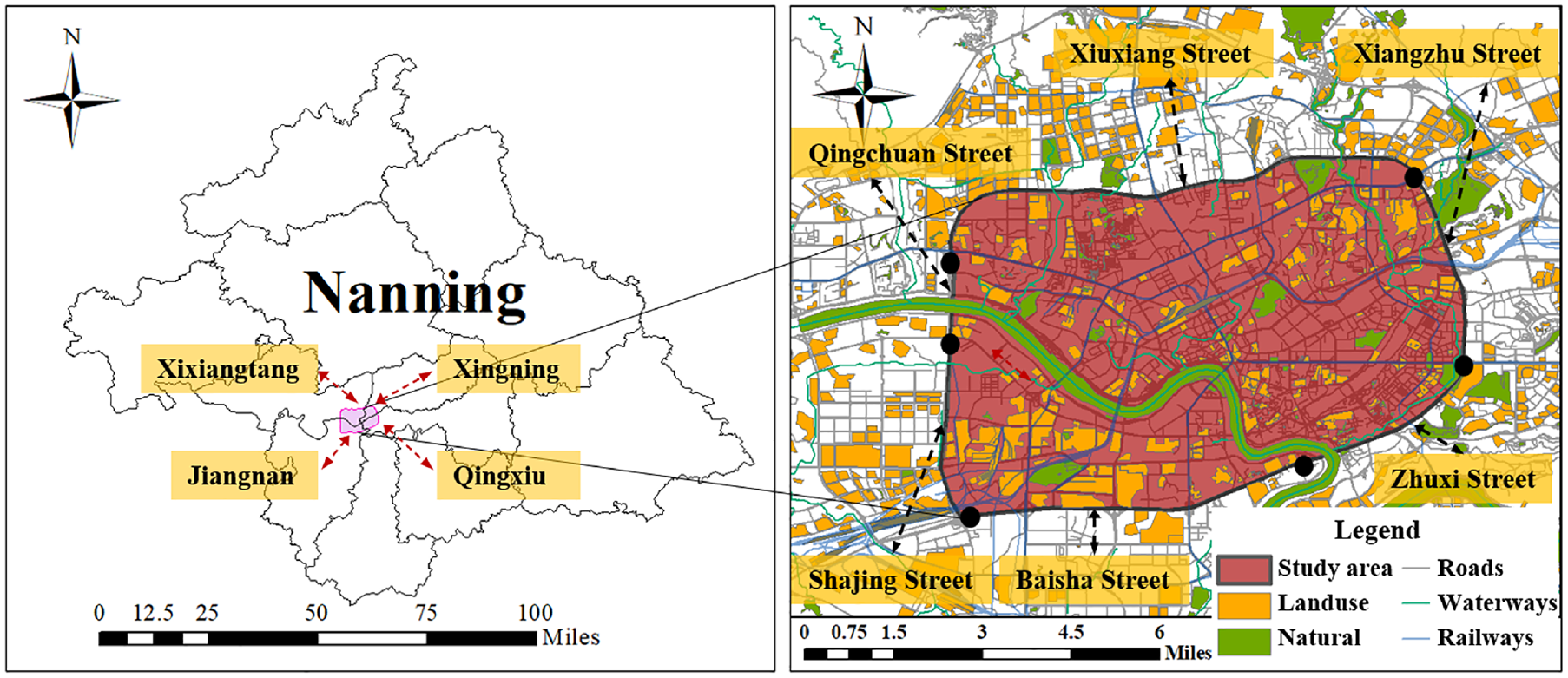
The schematic diagram of research area.
Data Source and Data Processing
The primary objective of this paper is to examine the nonlinear relationship between OCH travel demand and land use in different periods of time. There are three types of data used: OCH travel records, built environment, and road network information. Among them, the OCH travel data is from December 2, 2019 to December 8, 2019 in Nanning, with a total of 1,154,759 trips. A complete OCH travel order includes eight pieces of information: the order number (ID), the starting time, the starting longitude, the starting latitude, the ending time, the ending longitude, the ending latitude, and the distance, as presented in Table 2.
A Sequence of OCH Records
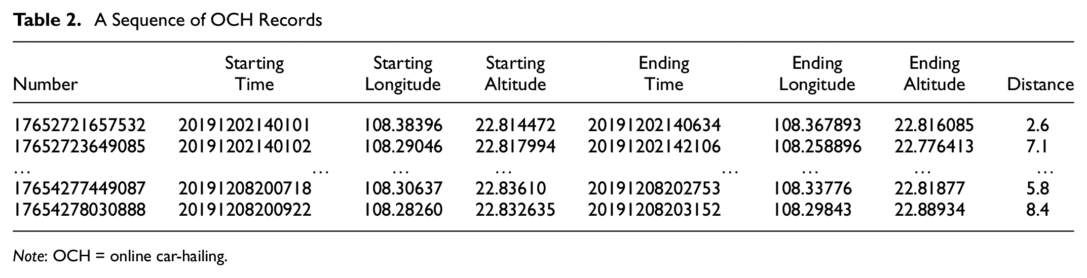
Note: OCH = online car-hailing.
Since some data cannot be used in this paper, data preprocessing needs to delete records that meet the following criteria: 1) the necessary information is missing; 2) the order number is repeated (the first occurrence of the record is retained); 3) the distance is less than 300 m; 4) the travel time is less than 1 min or more than 2 h; and 5) the latitude and longitude range exceeds the scope of Nanning. After filtering according to these rules, there were 1,136,203 pieces of valid data remaining. The road network used in this study can be obtained from the OpenStreetMap official website. A total of 210,000 POI data were obtained from Gaode’s map data open platform through Python, including the built environment of Nanning. In the field of transportation, POI data is a common source of data that can reflect the functional characteristics of an area to some degree. To avoid errors caused by subsequent data fusion, OCH travel data and POI data must simultaneously be transformed into the same coordinate system. The purpose of this paper is to analyze travel data in different time periods, so we count travel data per hour in this study, as shown in Figure 2.
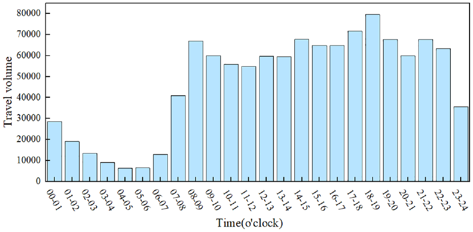
24-h travel data.
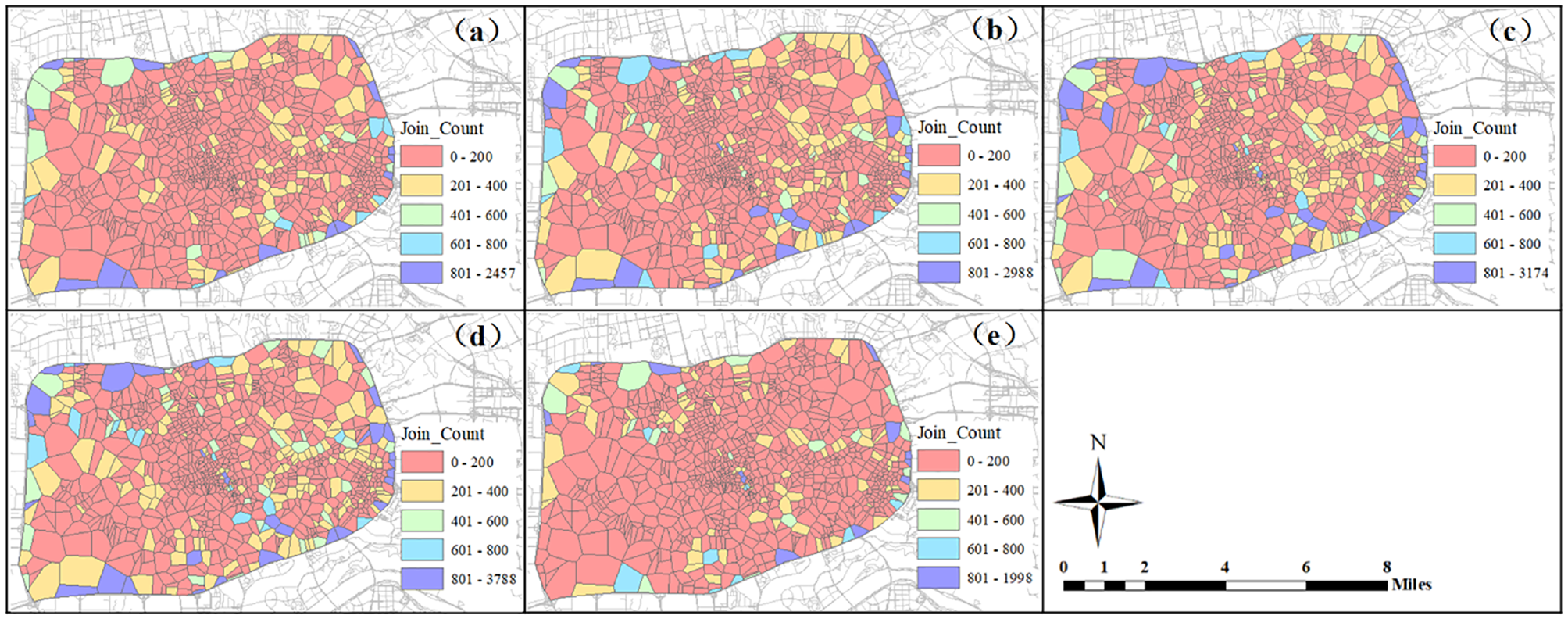
By taking into account the working hours of companies and the balance of travel during each time period, we divided the 24-h data into five time periods, namely 06:00 to 10:00, 10:00 to 14:00, 14:00 to 18:00, 18:00 to 22:00, and 22:00 to 02:00, to examine the nonlinear relationship between built environments and OCH travel demand during these five time periods. To obtain an overview of the travel situation within the research area, travel data were visualized on ArcGIS software, as shown in Figure 3.
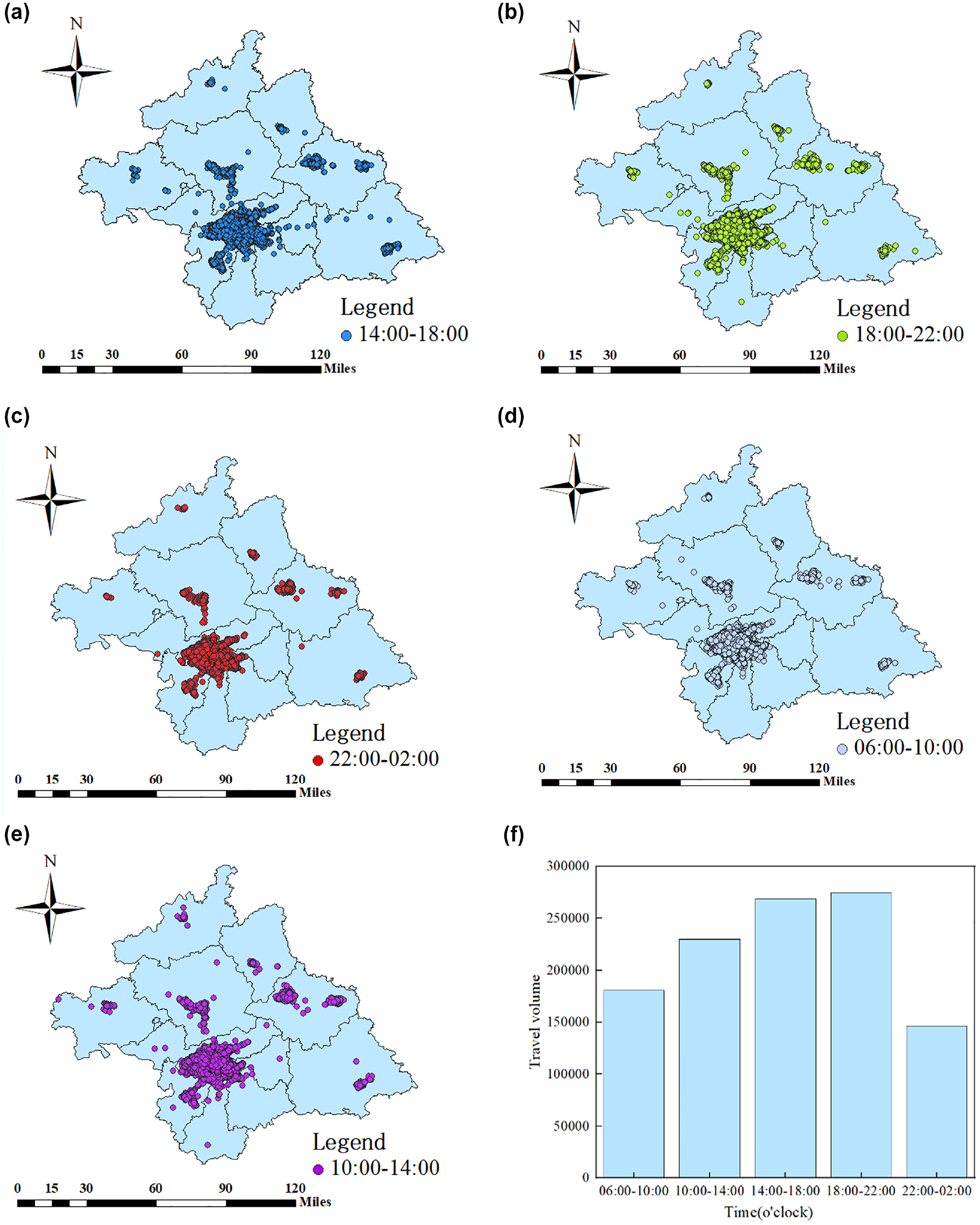
Spatial distribution of travel data in five periods and travel volume in five periods: (a) 14:00 to 18:00; (b) 18:00 to 22:00; (c) 22:00 to 02:00; (d) 06:00 to 10:00; (e) 10:00 to 14:00; and (f) travel volume in five periods.
As shown in Figure 3, a to e , the majority of OCH travel takes place in Nanning’s main urban area, with a noticeable spatial and temporal heterogeneity. From the perspective of travel volume (Figure 3f), however, there is no obvious peak during five periods, suggesting that OCH is not the main mode of transportation for residents of Nanning, contrary to our previous findings ( 38 , 39 ). Additionally, we must examine the nonlinear relationship between OCH trips and built environment in different periods more carefully by dividing the research area.
Methodology
Research Areas Division
To ensure the rationality of the refinement of the research areas, the research areas were further divided based on the structure of the road networks. The specific steps are as follows:
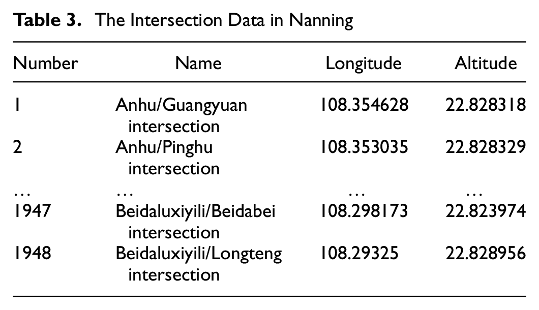
A complete record containing the intersection name, longitude, and latitude can be obtained by crawling the intersection data in Nanning through Python. Delete the intersection outside the research scope, and coordinates with longitude and latitude to form a finite set of points
The intersections (points) automatically construct Delaunay triangulation denoted as
Find and record the numbers of all triangles adjacent to each point, and find all triangles with one same vertex in the constructed triangulation.
The triangles adjacent to each discrete point are sorted clockwise or counterclockwise. The details are as follows: Take any point
Calculate the circumcircle center of each triangle in turn and record the center point set as
A Thiessen polygon is constructed based on the intersection of the circumcircle centers of the adjacent triangles surrounding each point. Each Thiessen polygon contains only one intersection, as shown in Figure 4.
The Intersection Data in Nanning
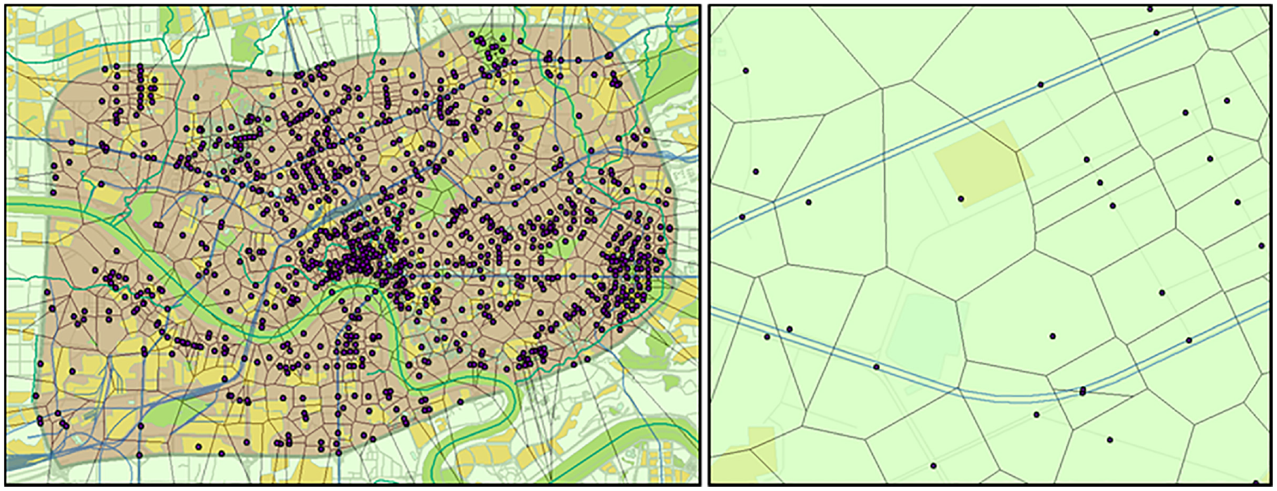
Thiessen polygons in research areas.
Random Forest
Based on the intersection Thiessen polygons, a random forest regression model was used to explore the potential impact of built environment on OCH travel demand in different periods.
The random forest model ( 40 ) is one of the most powerful ensemble learning algorithms for regression problems. It provides good performance in stability and correctness as a bagging ensemble model based on the classification and regression trees (CART) tree and has been widely used. To carry out effective ensemble learning, several weak classifiers are combined to create a strong classifier. To summarize, multiple decision trees are used to form a “forest” and the trees are classified by out-of-bag errors obtained from the voting results of multiple weak classifiers. A training set for out-of-bag estimation is derived by randomly placing back samples when building decision trees to establish a training set. This leads to a result where approximately 30% of the samples, referred to as out-of-bag data, are not used in the random forest generation process. The random forest model provides a way to compensate for overfitting when the data set contains many predictive variables, which can lead to complicated machine learning predictions. Furthermore, this model is capable of handling highly nonlinear variables and interactive variables, without the need for additional dummy variables, as well as ranking the contributions of each variable.
Given the discontinuous and non-monotonic nature of this technical approach, the random forest regression model can capture the detailed relationship between the built environment and the demand for OCH travel. And it can process continuous data and discrete data simultaneously. By using random forests, we can investigate the impact of various types of built environment elements on the OCH travel demand over time. Random forest adopts the bootstrap resampling method, which is composed of a series of decision tree models
The predicted value of random forest regression is the average value of
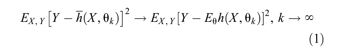
For all

where
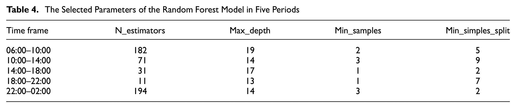
Various types and specifics of the built environment are the independent variables in the model. An OCH travel demand in the Thiessen polygon is the dependent variable for a complete record, which includes all POI types in that polygon as well as their corresponding data. To prevent overfitting and over complexity, it is necessary to select some super parameters for the random forest model. In five periods, the random forest model parameters were selected using the grid search method, as listed in Table 4.
The Selected Parameters of the Random Forest Model in Five Periods
The marginal effect of the prediction model can be estimated using the partial dependence plot of the machine learning model after the corresponding random forest model has been established. An analysis of the partial dependence plot is useful in determining the linear, monotonic, or complex relationship between objects and features. The partial dependence function of the regression is

where

where
Result and Discussion
Descriptive Analysis of Online Car-Hailing
(1) Duration. We conduct statistical analysis on the travel time of OCH in the research areas, as shown in Figure 5.
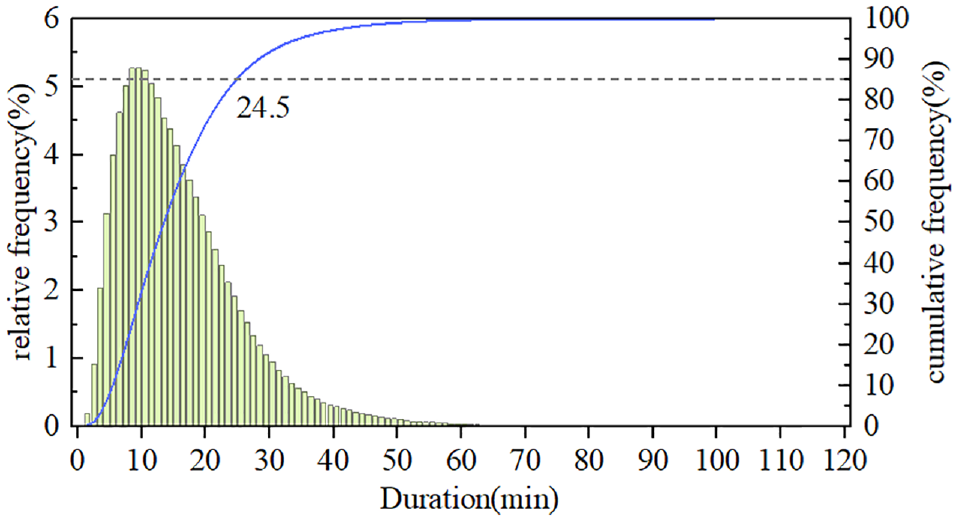
Distribution map of OCH travel time.
From Figure 5, it is evident that the service time for OCH trips in Nanning is mainly concentrated in 6 to 15 min. From the cumulative curve, it is also evident that 85% of travel users spend less than 24.5 min traveling. Furthermore, very few OCH services last longer than 50 min. Therefore, we can conclude from the above that most travel distances are less than 30 min for OCH, and thus, OCH may not be the best mode of transportation for long distances. When faced with a long-duration trip, people prefer to select other transportation modes instead of OCH given the higher cost ( 41 ). There are still some long-duration trips, however, which may result from the lack of other modes of transport or to avoid the traffic peak hours. Those passengers are willing to choose OCH instead of the metro as their first priority, and their second concern is avoiding the metro’s inconvenience resulting from the interchanges ( 41 ).
(2) Distance. We perform statistical analysis on the travel distance of OCH in the research areas, as shown in Figure 6.
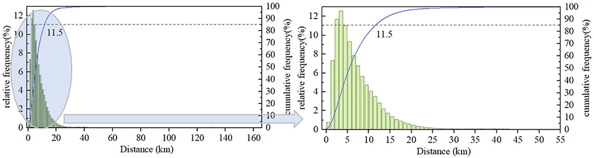
Distribution map of OCH travel distance.
From the distribution of OCH travel distance in Figure 6 we can see that the single travel distance of OCH in Nanning is mainly within the range of 2 to 7 km. According to the cumulative curve, 85% of users travel within 11.5 kilometers. Additionally, few users have a single service distance over 25 km, reflecting that users seldom use OCH for long-distance travel to some extent ( 23 ), which is perhaps a result of the high cost of long-distance travel.
(3) Space distribution. ArcGIS is used to visualize the spatial distribution of OCH in the research areas, as shown in Figure 7.
Spatial distribution of OCH travel demand: (a) 06:00 to 10:00, (b) 10:00 to 14:00, (c) 14:00 to 18:00, (d) 18:00 to 22:00, and (e) 22:00 to 02:00.
Hotspots in Figure 7a mainly involve Xingping Community, Dermatology Hospital and Textile Industry School, Jiangnan Xinxingyuan Community, Haotian Garden Community, Qingshan Community, Huayu Luyuan Community, and Guangxi University. We can find hotspots that are mainly composed of residential areas. Comparing Figure 7, a and b, there has been an increase in the points of presence of health care services, such as the People’s Hospital and First Affiliated Hospital of Medical University. Similarly, comparing Figure7, c and a , the study primarily increases leisure sport POIs, such as the first and second affiliated hospitals of Medical University, people’s hospitals, and zoos, while reducing some hotspots, such as residential areas. Compared with Figure 7c, Figure 7d mainly increases some leisure sport POIs, and reduces zoos and some health care POIs. The travel hotspot area of Figure 7e is significantly reduced.
Relationship Analysis
Built Environment Elements
To investigate the relevance of the demand for OCH, three main categories of built environment elements were selected for this study with reference to previous research findings ( 14 ). Specifically, home-work attributes ( 42 , 43 ), land use and diversity attributes ( 24 , 44 ), and traffic facility attributes ( 36 , 45 ). The importance of these three main categories of influencing factors has been confirmed in previous studies. In addition to the residential area, the home-work attribute includes the company. We have singled it out because commuting between the workplace and home is one of the key features of daily urban travel, and this commuting behavior has been identified as one of the key factors influencing OCH travel. There are two variables included in the traffic facility attribute: the subway station and the bus station. Among the parameters of the land use and diversity attribute, schools, government groups, hotels, health care, leisure sports, car services, motorcycle services, cultural services, financial insurance, shopping services, public facilities, scenic spots, catering services, and entropy are included. In total, 14 variables are included in this attribute. The descriptive statistics of the above 18 variables are listed in Table 5.
Descriptive Statistics of Independent Variables
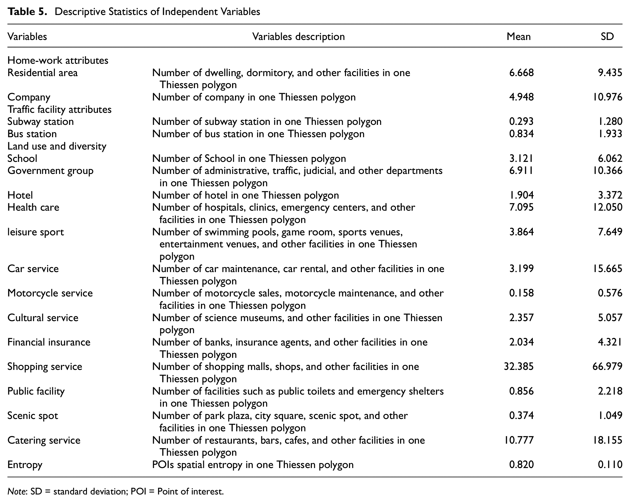
Note: SD = standard deviation; POI = Point of interest.
Importance of Independent Variables
The R2 values of the random forest model in the five periods of 06:00 to 10:00, 10:00 to 14:00, 14:00 to 18:00, 18:00 to 22:00 and 22:00 to 02:00 are 0.725, 0.776, 0.736, 0.780, and 0.703, respectively. These values indicate that the random forest model in this paper exhibits good prediction performance and can effectively capture the complex relationship between the built environment and OCH travel demand. The contribution and ranking of each variable in the prediction are presented in Table 6.
Importance Analysis of Independent Variables in Different Periods
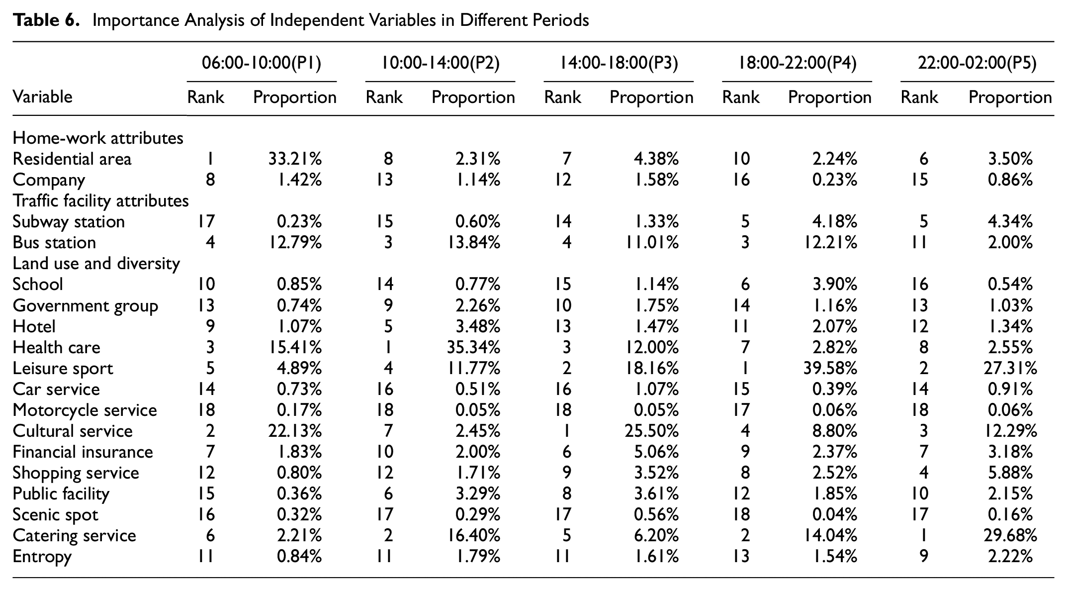
Table 6 indicates the impact of different built environment elements of OCH travel demand in different periods. The sum of relative importance of each independent variable is 100%. As a result of our research, different POIs in different periods contribute differently to the use of OCH, which is in contrast to our previous research findings. Previous studies suggest that the company and residential area play an important role in the use of OCH ( 21 ). According to the results, however, OCH use in residential areas is only significant for the period P1, with a contribution rate of 33.2%, while it is less than 5% for the other four periods. The company, which was valued in the past, contributed less than 5% in each period. This may be a result of Nanning residents often using electric bikes as travel tools. According to the results of the P1 analysis, 13 land use characteristics are responsible for about 50% of the prediction ability. Over 80% of the contributions were made in the remaining four periods. It is possible that this difference is a result of residents traveling for relatively single purposes during P1. There is a greater variety of travel purposes during the other four periods. For example, when traveling during other periods, it is more likely that travelers engage in varied activities such as catering, sports, and entertainment. There are four relatively important factors involved in land use: cultural services, health care, leisure sports, and catering services. In contrast to previous research conclusions, shopping services do not figure among them ( 14 ).
Furthermore, traffic facility attributes have a significant impact on OCH demand. However, five different periods occupy different positions in the model. According to the bus station, the contribution rates during P1, P2, P3, P4, P5 are 12.79%, 13.84%, 11.01%, 12.21%, and 2.00%, respectively. There is a contribution rate of less than 5% for the subway station over the five periods. Compared with subway stations, the impact of the bus station on OCH travel requirements is more obvious, indicating that people are more sensitive to existing bus services than subway services. Generally speaking, there is a greater contribution to OCH travel demand from the bus station than from the subway station. Over the course of the four periods, P1, P2, P3, and P4, the bus station has contributed significantly to OCH travel. There may be a reason for this, such as the inaccessibility of public transport which leads to the use of OCH, which is considered to be an important connection to public transportation ( 12 , 21 ). It is also possible that residents who originally planned to travel by public transportation gave up after waiting for an extended period of time and preferred OCH.
Nonlinear Impacts of Independent Variables
Based on the partial dependence plot generated by the random forest model, the nonlinear impacts of independent variables are identified. For analysis of the impact of built environment elements on OCH travel over time, all other independent variables have been set to constants. The partial dependence plot of home-work attribute is shown in Figures 8 and 9. The partial dependence plot of land use and diversity is shown in Figure 10, and traffic facility attribute is shown in Figure 11.
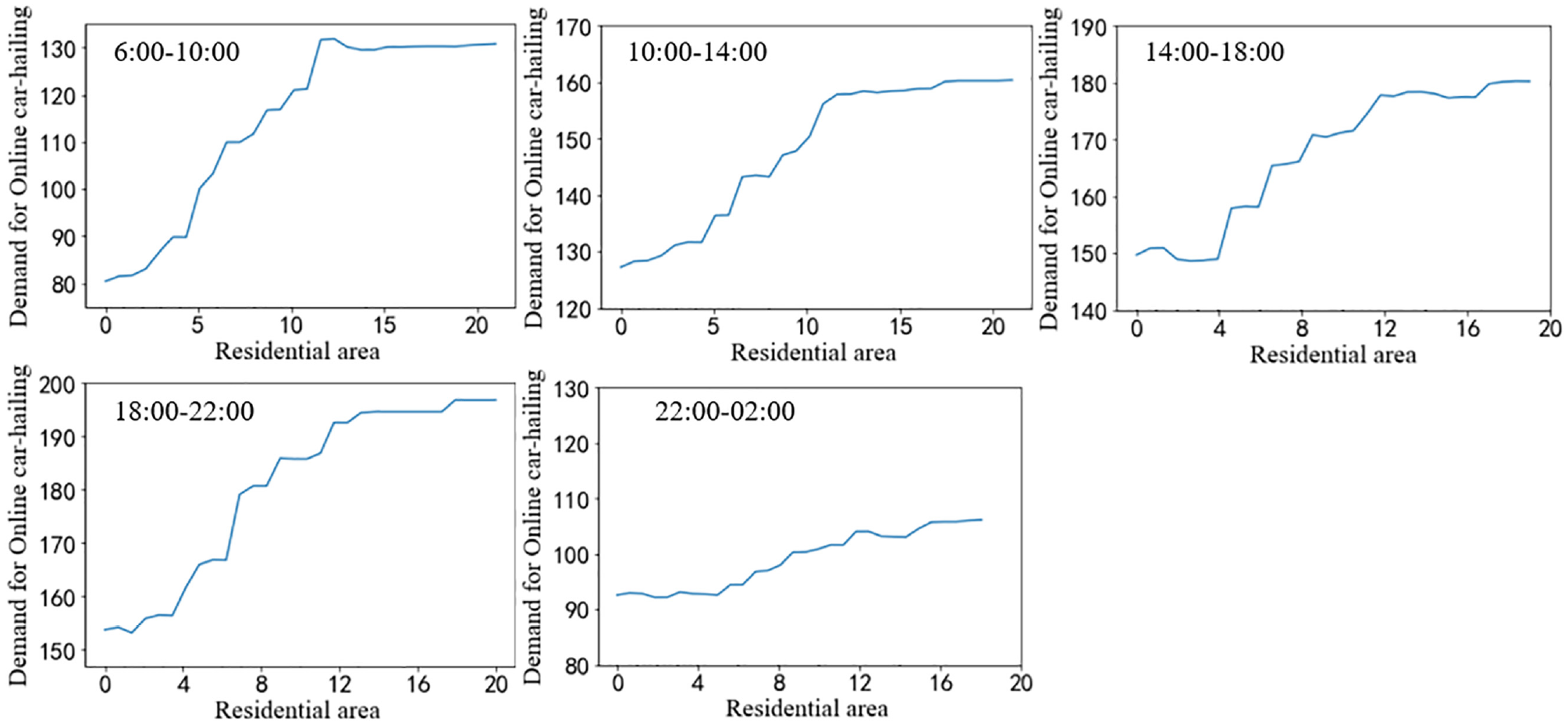
Nonlinear impacts of residential area in different periods on OCH travel demand.
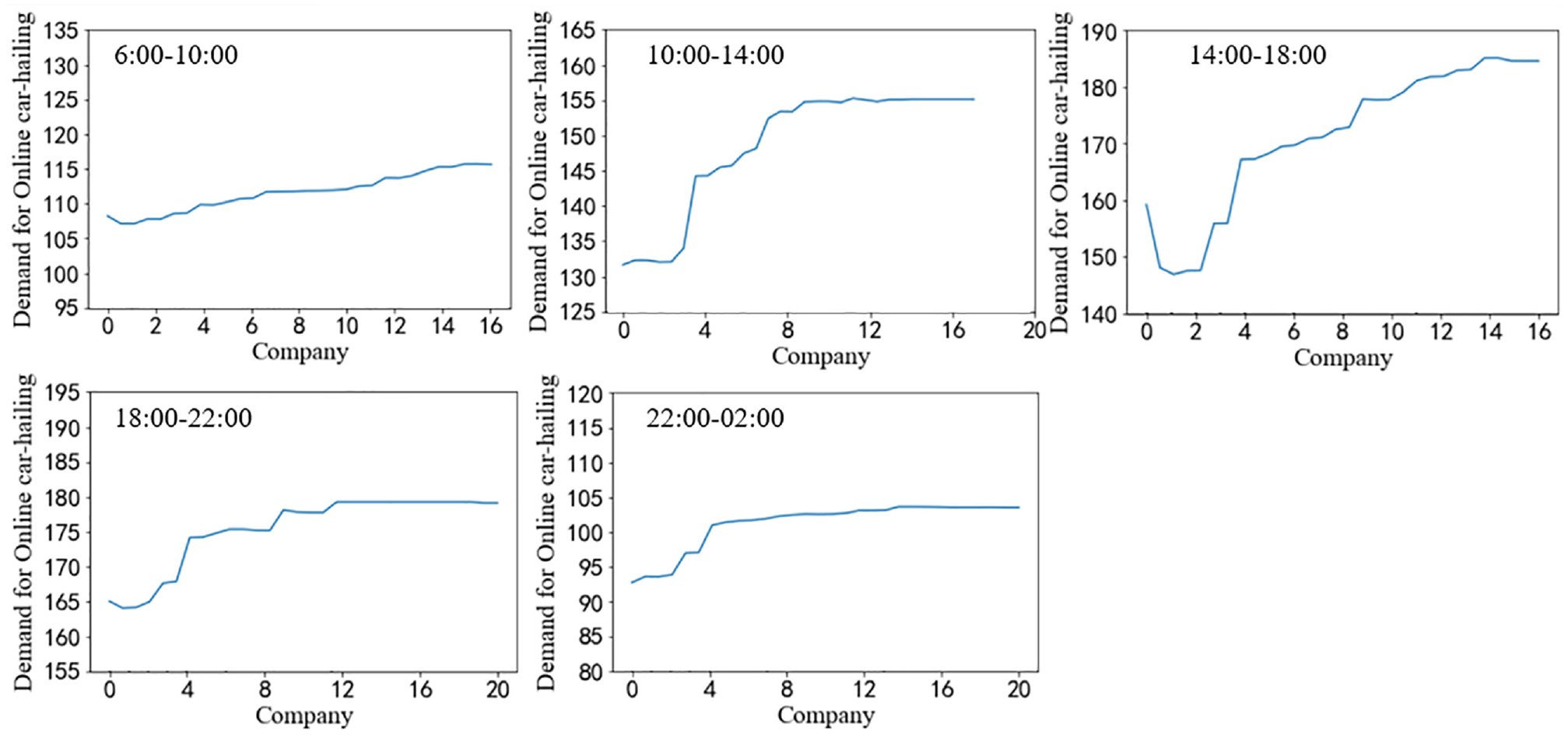
Nonlinear impacts of company in different periods on OCH travel demand.
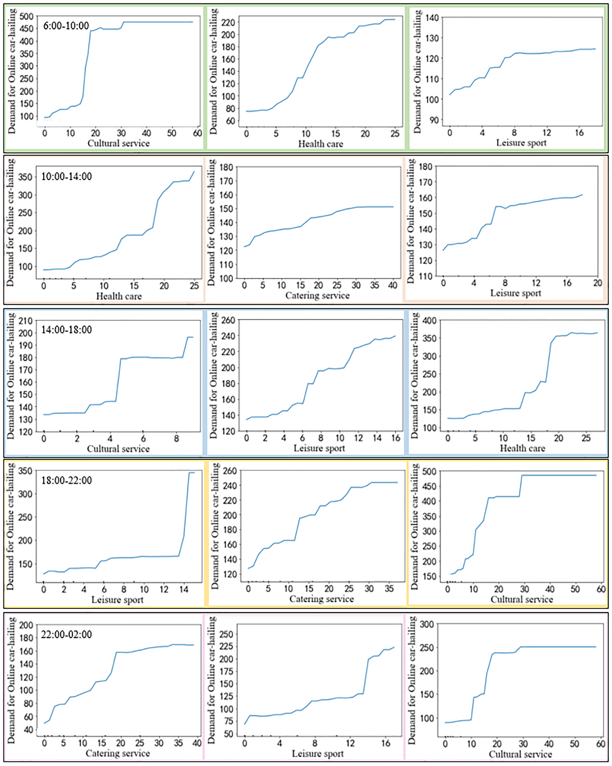
Nonlinear impacts of land use and diversity in different periods on OCH travel demand.
Nonlinear impacts of traffic facility attribute in different periods on OCH travel demand.
It can be seen from Figure 8 that there is a positive correlation between residential areas and OCH trips, which is consistent with previous research ( 12 ). However, it is readily apparent that for the period P1, when the number of residential areas in the fixed area increases from 0 to 12, there will be a significant increase (about 50 times) in OCH trip needs. Travel demand change will slow when there are more than 12 residential areas in a fixed area. In addition, during the other four periods, we can observe that when the residential areas are between 0 and 5, an increase in residential areas does not result in a significant increase in OCH trips. There is a significant impact elasticity of residential areas on OCH during the period of P1, about twice that of other periods.
As can be seen from Figure 9, there is a significant impact of increasing the number of company POIs on the use of OCH travel demand in P2 and P3, but not in P1, P4, or P5. There is a noticeable elastic relationship between the number of company POIs and OCH travel demand during the period of P2 and P3. There is a possibility that this is because most workers choose OCH to go out during their work hours. OCH can provide door-to-door service to meet workers’ timeliness requirements and enable them to complete their tasks before the end of the working day.
The 15 subgraphs in Figure 10 are the relationship between the three most important land-use variables and the corresponding OCH travel demand at different periods. According to Figure 10, the relationship between land-use variables and the demand for OCH travel is nonlinear during different periods. Additionally, all land-use variables have a positive impact on OCH travel in general, but the effects of each period may differ in magnitude. During the P1 period, the growth of cultural services from 0 to 15 had little effect on the demand for OCH. It has been shown that as the number of cultural services increases from 15 to about 20, the number of OCH travel services increases as well, reaching a steady value of about 450 times when there are about 20 cultural services. Cultural services mainly involve some training institutions. The results show that only a few training institutions fail to attract enough OCH trips. It should be noted, however, that when a region has enough training institutions and establishes its trading area in a city, it will have a profound impact on the need for OCH in that area. It is noteworthy that health care service is an important factor influencing the period of P2. There is little impact on the OCH demand when the number of health care services is less than five. In contrast, the number of OCH trips has increased by about 250 times when the number increased from 5 to 25. This may reflect most patients preferring to leave home early in the morning for treatment at hospital, so the end of treatment falls mostly during this time frame. As a consequence of physical discomfort, they prefer a more comfortable and quieter means of transportation, which significantly impacts the travel needs of OCHs in the health care area.
When the number of leisure sports services is between 0 and 6, it has little impact on demand during the period of P3. When the number increased from 6 to 16, the demand for OCH trips shows a sharp growth trend. Health care is also a major influencing factor during this period. The trend presented is consistent with period P2. The impact of health care service on OCH demand is a relatively new finding. There are three major land-use variables that affect OCH travel during the P4 and P5 periods: leisure sports, catering services, and cultural services. These two periods show a certain similarity in land-use variables related to OCH travel demand. It is possible that these two periods are both rest times for residents following a long day of work, so travel activities during these two periods are consistent. To effectively affect OCH needs during P4, the number of leisure sports services should reach at least 13. Meanwhile, the demand for OCH travel is not always affected by the catering service. There is a greater impact of catering during the P4 and P5 periods, whereas it is not a major factor during the daytime.
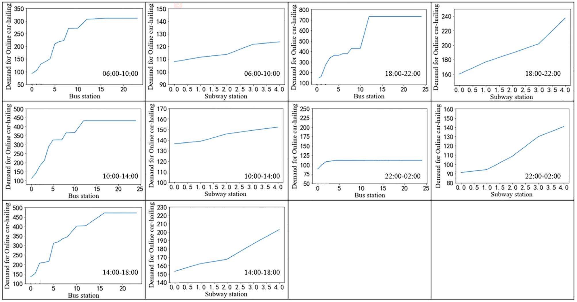
The impacts of traffic facilities in different periods on the use of OCH are shown in Figure 11. It is almost impossible to discern any impact from the number of bus stations on the amount of OCH travel demand during P5. In contrast, there is a significant positive elastic relationship between the number of bus stations and demand during the period P1∼P4. From the perspective of the five periods, the impact of bus stations on OCH demand reaches saturation around 15, indicating that bus stations have a limited impact on OCH demand. Generally speaking, the subway station has no negative impact on the demand for OCH, but it does not have a significantly positive impact at all times. For example, in the periods P1 and P2, the subway stations increased from 1 to 4, and the increase in the demand for OCH is about 20. In the three periods P3, P4, and P5, the subway system has a significant positive impact on OCH demand. The subway stations increased from 1 to 4, and the increase in OCH demand reaches about 50∼80. This indicates that the subway system has little effect on the demand during P1 and P2, while it has a significant impact on the demand for OCH during P4 and P5. This may be because most buses’ last bus time is about 22:00. Given the shutdown of bus lines during P4 and P5 at night, there is limited travel mode available in the last kilometer, and more individuals use the OCH to connect to the subway system ( 24 , 46 ). Furthermore, it indicates that there are few users who use OCH to connect to the subway in Nanning in the morning, and the subway system has a limited impact on OCH use. Based on this result, it appears that OCH and the subway system are capable of cooperating on service timing.
Conclusions and Policy Implications
From the micro perspective, this study examined the relationship between OCH travel and the built environment in different periods of time. Specifically, a comprehensive analysis of the balance between working hours in urban areas and travel during each period was conducted by dividing the research period into five categories (6:00–10:00, 10:00–14:00, 14:00–18:00, 18:00–22:00, 22:00–02:00). Furthermore, to obtain the correlation analysis unit, the research area division method was proposed based on intersection, and it was then combined with a random forest partial dependence plot to explore the impact of built environmental factors on OCH use over five typical periods. As a result of this study, we will further examine the mechanism by which built environment elements influence OCH demand in different periods, as well as discover the discontinuous and non-monotonic relationship between the two in different periods. It provides results useful for follow-up research, as follows:
In different periods, OCH travel demand may differ as a result of heterogeneity in the built environment. According to some theories, this phenomenon is potentially caused by there being an inverse correlation between the purpose of urban residents’ travel and the time of their travel, which results in an uneven distribution of their travel demand over time and space. First of all, results show that residential areas, which have always been highly valued, have a significant influence on OCH travel demand during the period P1, with a contribution rate of 33.2%, while the predicted contribution rates for the remaining four periods are less than 5%. To prevent excessive invalid no-load patrolling, a decline in order receiving rates, and meaningless exhaust emissions, the OCH and taxi management department must control the vehicles patrolling near the residential area in the other four periods. In contrast, the contribution rate of the company to the OCH requirements in Nanning has been below 5% in five periods, which is significantly different from previous studies. Secondly, generally speaking, there is a greater contribution to OCH travel demand from the bus station than from the subway station. Specifically, there was a significant contribution rate of more than 10% for the bus station in the four periods P1 through P4, and the contribution rate in the period P5 was less than 5% for the subway station. The results confirm that passengers who planned to travel by bus during P1 to P5 may be disappointed with the bus service given long waiting times or crowded bus passenger flow, and instead turn to OCH. Furthermore, it demonstrates the potential to connect OCH and buses in Nanning.
In addition, the nonlinear relationship between land-use variables and demand for OCH trips varies at different times of the day and has different threshold effects. The contribution of land-use attributes to the demand varies between time periods, and the main influencing variables differ. Specifically, during P1 only about 50% of OCH travel demand was attributed to land use and diversity attributes. During the other four periods, the contribution exceeded 80%. Among these 13 attribute variables, cultural service, health care service, leisure sport service, and catering service are four relatively important factors, which apply to five different time periods. A major contribution comes from cultural services in P1 and P3. It is important to note, however, that in cases where there are enough training institutions to form a separate trading area within a city, this may have a profound impact on the OCH travel demand. In contrast, the contribution of health care services is the most important of the land-use variables in the P2 period, which is a relatively new finding. But it also has a certain threshold effect, when the number of health care services in the study unit is less than 5, the effect on OCH demand is small. When the number increased from 5 to 25, the number of trips made by the OCH increased by a factor of about 250. For the P4 and P5 periods, the main land-use variables are also more similar because of some similarities in the purpose of the trips. Leisure sports services and catering services make up the majority of the contributions in periods P4 and P5. Catering service, which was the focus of previous studies ( 12 , 24 ), did not always greatly affect the demand for OCH, such as P1 and P3 periods.
This paper provides effective guidance for the scheduling of urban occupational health and safety services. To improve cruising efficiency and reduce waiting times for residents, traffic guidance and scheduling are effective methods to recommend routes that are in high demand to OCH drivers. It is important to note that these findings are of great importance to other cities around the world that have similar travel habits and structures to Nanning. Secondly, to reduce the interference between static traffic and dynamic traffic flow for the main contribution POI types in different periods, the government may adopt some necessary traffic organization and control measures, such as optimizing the parking area at the OCHs to reduce the interference caused by static traffic. Thirdly, when there are high traffic levels in some areas, it would be helpful to check the quality of the operation of the bus lines, to avoid residents becoming dissatisfied with public transportation services and turning to OCH travel, resulting in higher levels of traffic. Finally, since the built environment and OCH travel display heterogeneous and nonlinear relationships in different periods, relevant policies can be developed according to the scale characteristics of urban infrastructure. Meanwhile, the balance between supply and demand of transportation facilities in high-demand areas of the built environment is adjusted to promote sustainable development of public transportation.
Although our work is a comprehensive study that explores the nonlinear effects of the built environment on the demand for OCH travel on a time scale, there are still some limitations that require further research. First, the independent variables studied in this paper do not have access to data related to sociodemographic and service factors (ease of use) given data limitations. These factors may be co-linear with some land-use types and thus have an impact on the demand. Secondly, this study is limited to data on pick-up points for OCH trips, while no relevant research has been conducted on the distribution of drop-off points, and a subsequent comparison of pick-up and drop-off points could be interesting. Thirdly, to capture the nonlinear relationship between the built environment and the demand for OCH, this study focuses more on interpreting the machine learning results to provide some policy guidance to relevant departments, which is why it uses only the random forest model. To understand why different machine-learning models differ, it might be helpful to pay attention to the differences between some of them. Then, considering that in many countries car-hailing is not integrated with other transport modes, our approach can be extended to ride-hailing more generally. So exploring the relationship between the built environment and on-demand buses and minibuses could be a good direction to take in the future. Last but not least, given space constraints, we have not compared weekdays and weekends, and it will be interesting to compare and analyze the model performance on weekdays and weekends in future studies to find the differences.
Footnotes
Author Contributions
The authors confirm contribution to the paper as follows: study conception and design: X. Zhou, Y. Ji; data collection: X. Zhou, M. Lv, Y. Ji; analysis and interpretation of results: X. Zhou, M. Lv; draft manuscript preparation: X. Zhou, M. Lv, Y. Ji. All authors reviewed the results and approved the final version of the manuscript.
Declaration of Conflicting Interests
The author(s) declared no potential conflicts of interest with respect to the research, authorship, and/or publication of this article.
Funding
The author(s) disclosed receipt of the following financial support for the research, authorship, and/or publication of this article: This research was funded by the National Key R&D Program of China (2018YFB1600900).
Data Availability Statements
Given the nature of this research, the data provider requested that the data be kept confidential, so supporting data is not available.